Iron and nickel atoms in cometary atmospheres even far from the Sun
←
→
Page content transcription
If your browser does not render page correctly, please read the page content below
Iron and nickel atoms in cometary
                    atmospheres even far from the Sun
                         J. Manfroid, D. Hutsemékers, and E. Jehin
                             STAR Institute, University of Liège
                         Allée du 6 Août 19c, B-4000 Liège Belgium

                                        February 02, 2020

Abstract

In comets, iron and nickel are found in refractory dust particles or in metallic and sulfide
grains1. No iron- or nickel-bearing molecules have been observed in the gaseous coma of
comets2. Iron and a few other heavy atoms such as copper and cobalt were only observed in
two exceptional objects, the Great Comet of 18823 and, almost a century later, C/1965 S1
(Ikeya-Seki) 4-9 . These sungrazing comets approached the Sun so close that the refractory
materials could sublimate. The relative abundance of nickel to iron was similar to the Sun
and the meteorites7. More recently the presence of iron vapor was inferred from the
properties of a faint tail in comet C/2006 P1 (McNaught) at perihelion 10 but neither iron nor
nickel was reported in the gaseous coma of comet 67P/Churyumov-Gerasimenko by the in
situ Rosetta mission11. Here we report that neutral FeI and NiI emission lines are ubiquitous
in cometary atmospheres, even far from the Sun, as revealed by high-resolution UV-optical
spectra of a large sample of comets of various compositions and dynamical origins. The
abundances of both species appear to be of the same order of magnitude, contrasting the
typical Solar System abundance ratio.

The spectra of about 20 different comets were collected since 2002 over a large range of
heliocentric distances (0.68 to 3.25 astronomical units) with the UVES spectrograph mounted
on the 8-m UT2 telescope of the ESO Very Large Telescope (Extended Data, Table 1). The use of
a dichroic beam splitter and a narrow 0.4" slit provided a resolving power (λ/∆λ) of about 80000 over
the wavelength range 304-1040 nm. The slit length of ~10" typically covers ~7500 km of the coma
at a distance of 1.0 au and except for a few cases the slit was centered on the comet nucleus. A
uniform procedure12 has been used for the acquisition and the reduction of all the data.
Close examination of these spectra revealed the omnipresence of emission lines of neutral atoms
of iron (FeI) and nickel (NiI) in comets as far as 3.25 au from the Sun with up to about 40 FeI lines
and 25 NiI lines for some of them (Extended data, Fig. 1). These lines are weak and located in the
blue part of the spectrum (< 450 nm) where there are plenty of bright molecular emissions making
blends unavoidable, explaining in part why they were missed until now. We searched for the lines of
the other metals that were identified in comet Ikeya-Seki 7,8, in particular neutral chromium, the most
abundant after nickel, but we did not find any of them. NiI lines were recently identified in the
                                                   1
interstellar comet 2I/Borisov (Guzig & Drahus, this issue).
The metallic lines, contrary to the molecular lines, have only a short spatial extension as it was
already noted for Ikeya-Seki7, despite very different conditions of temperature and irradiation. The
few spectra not centered on the nucleus do not show these lines, or only faintly. In the spectra
obtained during the close encounter of comet 103P/Hartley 2 with the Earth (Figure 1), these lines
show a radiance inversely proportional to the projected distance to the nucleus p. Such a profile
corresponds to an ejection from the surface of the nucleus or a short-lived parent5 and a constant
expansion velocity, resulting in a p-2 density distribution. The spectra taken at various position
angles indicate that the metals distribution in the inner coma is nearly isotropic, which suggests
collisional dragging and an initial velocity high enough to hide radiative pressure effects.
Once freed in a collision-less environment, the atoms are bathed into the solar radiation and would
conceivably tend toward an excitation temperature of the order of the color temperature of the Sun,
about 5800 K. In order to analyze their emission spectra, we first considered a simple 3-level
atomic model as done previously for the analysis of Ikeya-Seki4,13. We then built a more realistic
multilevel atomic model taking into account the high-resolution structure of the solar spectrum
(Supplementary Information). This allowed us to compute the production rates of NiI and FeI for
each comet. In the case of an isotropic expansion at a constant velocity v, the column densities
C(p) and the production rates Q are linked by the relation C(p) = Q(4v∆p)−1, where ∆ is the
geocentric distance. The observed average density over the slit area A is N = Q(4v∆A)−1 ∫A p-1 da.
Due to the atmospheric blurring, we used instead the convolution of the 1/p profile with a 1"
Gaussian. We adopted the commonly assumed value of v = 0.85 r−1/2 km/s for the expansion
velocity14. Extended Data Table 2 gives for each spectrum the FeI and NiI column densities and the
corresponding production rates. The quantities found are very small. For the Jupiter family comet
103P they correspond to only ~1 g of iron ejected every second, compared to ~100 kg of water,
making these elements minor constituents of the coma.
To compare these abundances to the other usual species observed in comets, we derived from our
spectra the production rates of the radicals OH (a daughter product of water), CN and CO2+
(Extended DataTable 3), and collected CO and H2O IR and submillimeter measurements from the
literature. Figure 2 of Extended Data shows that the abundances of iron and nickel atoms are well
correlated with the other species and the comets activity level. Of particular interest is the high
metallic abundance in the distant and chemically peculiar comet C/2016 R2 relative to its other
elements, except CO and CO2+. This suggests a possible link between Fe, Ni and the carbon
oxides. This water-poor comet had a high activity driven by a large CO production rate of about
1029 molecules/s at ~3 au15,16.
The average NiI/FeI abundance ratio is about unity (log(Ni/Fe) = -0.06 ± 0.31), i.e., an order of
magnitude higher than the solar value 17 (−1.25 ± 0.04) or the ratio measured in comet Ikeya-Seki
(−1.11±0.09) and it does not depend on the heliocentric distance or the comet origin. In our sample,
comet 103P has the lowest value (−0.64±0.07), and the carbon-chain depleted comet 73P the
highest value (0.60±0.23), both at heliocentric distances r~1 au (Fig. 2).
2The comet black-body equilibrium temperature of its surface is expected to be around T ~ 280 r−1/2
K with r in au, that is ~340 K for the comet observed at the closest distance to the Sun (0.68 au)
and ~150 K for the most distant one (3.25 au). These temperatures are much lower than those
needed to vaporize refractory dust grains as well as iron and nickel in metallic form or in sulfides 10.
We thus explore several possibilities to explain how Fe and Ni atoms are released at such low
temperatures and why the Ni/Fe ratio is enhanced.
The β-parameter characterizing the ratio between the radiation pressure and the gravity, which is
about 6 for iron10, is too small to alter substantially the velocity field in the vicinity of the nucleus and
decrease the column density of iron relative to nickel. Moreover, comet Ikeya-Seki which should
show the largest effects, displays a normal (solar) abundance ratio. The high Ni/Fe ratio observed
must then be representative of the sublimating material or the sublimation process.
Iron in meteorites is known to be distributed between silicates, sulfides and metallic iron, silicates
and metallic iron requiring higher temperatures (~1200 K) to sublimate than sulfides (~600 K), while
nickel is only found in sulfides and the metal phase 18,19. We may thus expect a higher Ni/Fe ratio if
sublimation occurs at temperatures lower than 1000 K. This is supported by the fact that FeNi
alloys and sulfides formed in the low temperature range are Ni-rich, such as kamacite and
pentlandite20. Although some comets may actually be Ni-rich, partial sublimation of such species
could explain the high Ni/Fe ratios we measure in comets far enough from the Sun. Fe and Ni as
well as Ni-rich sulfides like pentlandite have been found in cometary material and interplanetary
dust particles (IDPs), often in the form of nanometer-sized particles 21–23. The number of Fe and Ni
atoms being the same in such compounds, it would offer an explanation for the relative abundance
close to one, in average, but not the large over- or under-abundance of NiI, observed in, e.g.,
comets Garradd and 103P, or in the carbon-chain depleted comets 21P and 73P. This interpretation
requires temperatures above approximately 600 K, still higher than expected at heliocentric
distances larger than 0.4 au. However, small grains can be heated at temperatures higher than
blackbody equilibrium temperatures, e.g. superheating of submicrometer-sized fluffy aggregates 24.
Even higher temperatures can be reached for smaller grains, like metallic nanoparticles 25. Collisions
of high-velocity nanoparticles with cometary dust grains could break the matrix in which Fe and Ni
are embedded and produce impact vapor with a temperature of the order of 1000 K 26. Several
mechanisms can thus potentially provide the necessary heating, especially if a significant amount
of iron and nickel is in the form of nanoparticles. The refractory elements Na, K, Si, and Ca have
been found by the Rosetta spacecraft in the gaseous coma of 67P at large distance from the Sun (3
au) and attributed to ion-induced sputtering of the nucleus surface material by the solar wind, but
Fe and Ni have not been reported 27. We do not observe the light refractory elements in our spectra,
and nucleus sputtering would not be active for comets closer to the sun due to the much denser
coma and would not produce the correlations between Fe, Ni and the other volatile species that we
observed (Extended data, Fig. 2).
Organometallic complexes such as [Fe(PAH)] +, carbonyls like Fe(CO)5 and Ni(CO)4, and even iron
pseudocarbynes, have been proposed as possible constituents of cometary or interstellar
material28–31. The strong correlation of the production rates of iron, nickel and carbon oxides for all
the comets of our sample led us to evaluate the possibility of the carbonyl hypothesis. We
3estimated the sublimation temperatures and sublimation rates of both Fe and Ni carbonyls
(Extended Data Fig. 3). These temperatures are only slightly higher than that of CO 2 and indicate
that, if present in comets, these carbonyls can sublimate at low temperatures and at large distances
from the Sun, contrary to silicates and sulfides. This could explain why carbonyls have not been
found in IDPs while they have been recently identified in the Lewis Cliff 85311 meteorite 32.
Furthermore the higher rate of sublimation of Ni(CO) 4 compared to Fe(CO)5 (Extended Data Fig. 3),
about a factor 10 at temperatures around 300 K, typical of the diurnal temperature of the nucleus 33,
might provide a simple explanation to the Ni/Fe overabundance, although this scenario depends on
the efficiency of the photo-dissociation of the carbonyls. Interestingly, similar computations for Cr,
the next most abundant metal in the Sun after Ni, show that the sublimation rate of Cr(CO) 6 is lower
by a factor of ~100 with respect to Fe(CO) 5, which means that CrI would be a factor ~10000 less
abundant than FeI, explaining the non-detection of the CrI lines. A detailed photo-chemical model
analysis, beyond the scope of this paper, would be needed to verify if this scenario can actually
reproduce the measured abundances, but the discovery of iron and nickel free atoms in comets
indicates that important constituents of the nucleus or processes in the coma are still missing,
possibly bringing new important constraints on comets composition and the Solar System
formation.
References
1. Zolensky, M. E. et al. Mineralogy and Petrology of Comet 81P/Wild 2 Nucleus Samples. Science
314, 1735 (2006).
2. Bockelée-Morvan, D. & Biver, N. The composition of cometary ices. Philos. Trans. R. Soc. Lond.
Ser. A 375, 20160252 (2017).
3. Copeland, R. & Lohse, J. G. Spectroscopic observations of comets III and IV, 1881, comet I,
1882, and the Great Comet of 1882. Copernic. Int. J. Astron. 2, 225–244 (1882).
4. Arpigny, C. Relative abundances of the heavy elements in comet Ikeya-Seki /1965 VIII/. in Liege
International Astrophysical Colloquia (eds. Boury, A., Grevesse, N. & Remy-Battiau, L.) vol. 22
189–197 (1979).
5. Combi, M. R., DiSanti, M. A. & Fink, U. The Spatial Distribution of Gaseous Atomic Sodium in the
Comae of Comets: Evidence for Direct Nucleus and Extended Plasma Sources. ıcarus 130, 336–
354 (1997).
6. Dufay, J., Swings, P. & Fehrenbach, Ch. Spectrographic Observations of Comet Ikeya-Seki
(1965f). Astrophys. J. 142, 1698 (1965).
47. Preston, G. W. The spectrum of Ikeya-Seki (1965f). Astrophys. J. 147, 718–742 (1967).
8. Slaughter, C. D. The Emission Spectrum of Comet Ikeya-Seki 1965-f at Perihelion Passage.
Astron. J. 74, 929 (1969).
9. Thackeray, A. D., Feast, M. W. & Warner, B. Daytime Spectra of Comet Ikeya-Seki Near
Perihelion. Astrophys. J. 143, 276 (1966).
10. Fulle, M. et al. Discovery of the Atomic Iron Tail of Comet MCNaught Using the Heliospheric
Imager on STEREO. Astrophys. J. Lett. 661, L93–L96 (2007).
11. Kathrin Altwegg and the ROSINA Team. Chemical highlights from the Rosetta mission.
Astrochemistry VII – Through the Cosmos from Galaxies to Planets, Proceedings IAU
Symposium No. 332 (2017).
12. Arpigny, C. et al. Anomalous Nitrogen Isotope Ratio in Comets. Science 301, 1522–1525
(2003).
13. Arpigny, C. On the nature of comets. In Proceedings of the Robert A. Welch Foundation
Conferences on Chemical Research XXI, Cosmochemistry (ed. Mulligan, W. O.) 9 (1978).
14. Cochran, A. L. & Schleicher, D. G. Observational Constraints on the Lifetime of Cometary
H2O. ıcarus 105, 235–253 (1993).
15. Biver, N. et al. Long-term monitoring of the outgassing and composition of comet
67P/Churyumov-Gerasimenko with the Rosetta/MIRO instrument. Astron. Astrophys. 630, A19
(2019).
16. Womack, M., Sarid, G. & Wierzchos, K. CO in Distantly Active Comets. Publ. Astron. Soc.
Pac. 129, 031001 (2017).
17. Lodders, K. Solar Elemental Abundances.
https://doi.org/10.1093/acrefore/9780190647926.013.145 (2020).
18. Larimer, J. W. & Anders, E. Chemical fractionations in meteorites - III. Major element
fractionations in chondrites. Geochim. Cosmochim. Acta 34, 367–387 (1970).
19. Grossman, L. & Larimer, J. W. Early chemical history of the solar system. Rev. Geophys.
Space Phys. 12, 71–101 (1974).
20. Lewis, J. S. Physics and chemistry of the solar system. 2nd Edition. (2004).
521. Berger, E. L., Zega, T. J., Keller, L. P. & Lauretta, D. S. Evidence for aqueous activity on
comet 81P/Wild 2 from sulfide mineral assemblages in Stardust samples and CI chondrites. Geo.
Cosmo. Acta 75, 3501–3513 (2011).
22. Bradley, J. P. Chemically Anomalous, Preaccretionally Irradiated Grains in Interplanetary
Dust From Comets. Science 265, 925–929 (1994).
23. Ishii, H. A. et al. Comparison of Comet 81P/Wild 2 Dust with Interplanetary Dust from
Comets. Science 319, 447 (2008).
24. Bockelee-Morvan, D. et al. Comet 67P outbursts and quiescent coma at 1.3 au from the
Sun: dust properties from Rosetta/VIRTIS-H observations. Mon. Not. R. Astron. Soc. 469, S443–
S458 (2017).
25. Hensley, B. S. & Draine, B. T. Thermodynamics and Charging of Interstellar Iron
Nanoparticles. Astrophys. J. 834, 134 (2017).
26. Ip, W.-H. & Jorda, L. Can the Sodium Tail of Comet Hale-Bopp Have a Dust-Impact Origin?
Astrophys. J. Lett. 496, L47–L49 (1998).
27. Wurz, P., et al. Solar wind sputtering of dust on the surface of 67P/Churyumov-Gerasimenko.
Astron. Astrophys. 583, p.A22 (2015)
28. Bloch, M. R. & Wirth, H. L. Abiotic organic synthesis in space. Naturwissenschaften 67, 562–
564 (1980).
29. Klotz, A. et al. Possible contribution of organometallic species in the solar system ices.
Reactivity and spectroscopy. Planet. Space Sci. 44, 957–965 (1996).
30. Huebner, W. F. Dust from cometary nuclei. Astron. Astrophys. 5, 286–297 (1970).
31. Tarakeshwar, P., Buseck, P. R. & Timmes, F. X. On the Structure, Magnetic Properties, and
Infrared Spectra of Iron Pseudocarbynes in the Interstellar Medium. Astrophys. J. 879, 2 (2019).
32. Smith, K. E., House, C. H., Arevalo, R. D., Dworkin, J. P. & Callahan, M. P. Organometallic
compounds as carriers of extraterrestrial cyanide in primitive meteorites. Nat. Commun. 10, 2777
(2019).
33. Prialnik, D., Benkhoff, J. & Podolak, M. Modeling the structure and activity of comet nuclei. in
Comets II (eds. Festou, M. C., Keller, H. U. & Weaver, H. A.) 359 (2004).
634. Levison, H. F. Comet Taxonomy. in Completing the Inventory of the Solar System (eds.
Rettig, T. & Hahn, J. M.) vol. 107 173–191 (1996).
35. A’Hearn, M. F., Schleicher, D. G., Millis, R. L., Feldman, P. D. & Thompson, D. T. Comet
Bowell 1980b. Astron. J. 89, 579–591 (1984).
36. Schleicher, D. G. The Fluorescence Efficiencies of the CN Violet Bands in Comets. Astron. J.
140, 973–984 (2010).
37. Schleicher, D. G. & A’Hearn, M. F. The Fluorescence of Cometary OH. Astrophys. J. 331,
1058 (1988).
38. Bhardwaj, A. & Raghuram, S. A Coupled Chemistry-emission Model for Atomic Oxygen
Green and Red-doublet Emissions in the Comet C/1996 B2 Hyakutake. Astrophys. J. 748, 13
(2012).
39. Raghuram, S. et al. A physico-chemical model to study the ion densitydistribution in the inner
coma of comet C/2016 R2(Pan-STARRS). ArXiv E-Prints arXiv:2012.04611 (2020).
40. Weaver, H., Feldman, P., A’Hearn, M., Dello Russo, N. & Stern, A. Comet 103P/Hartley. Iau
circ 9183, 1 (2010), https://ui.adsabs.harvard.edu/abs/2010IAUC.9183....1W.
41. Roth, N. X. et al. Probing the Evolutionary History of Comets: An Investigation of the
Hypervolatiles CO, CH4, and C2H6 in the Jupiter-family Comet 21P/Giacobini-Zinner. Astron. J.
159, 42 (2020).
42. DiSanti, M. A. et al. Depleted Carbon Monoxide in Fragment C of the Jupiter-Family Comet
73P/Schwassmann-Wachmann 3. Astrophys. J. Lett. 661, L101–L104 (2007).
43. Böhnhardt, H. et al. The Unusual Volatile Composition of the Halley-Type Comet 8P/Tuttle:
Addressing the Existence of an Inner Oort Cloud. Astrophys. J. Lett. 683, L71 (2008).
44. Lupu, R. E., Feldman, P. D., Weaver, H. A. & Tozzi, G.-P. The Fourth Positive System of
Carbon Monoxide in the Hubble Space Telescope Spectra of Comets. Astrophys. J. 670, 1473–
1484 (2007).
45. DiSanti, M. A. et al. Detection of Formaldehyde Emission in Comet C/2002 T7 (LINEAR) at
Infrared Wavelengths: Line-by-Line Validation of Modeled Fluorescent Intensities. Astrophys. J.
7650, 470–483 (2006).
46. Paganini, L. et al. Observations of Comet C/2009 P1 (Garradd) at 2.4 and 2.0 AU before
Perihelion. in Asteroids, Comets, Meteors 2012 vol. 1667 6331 (2012).
47. Paganini, L. et al. The Unexpectedly Bright Comet C/2012 F6 (Lemmon) Unveiled at Near-
infrared Wavelengths. Astron. J. 147, 15 (2014).
48. Biver, N. et al. The extraordinary composition of the blue comet C/2016 R2 (PanSTARRS).
Astron. Astrophys. 619, A127 (2018).
49. Wierzchos, K. & Womack, M. C/2016 R2 (PANSTARRS): A Comet Rich in CO and Depleted
in HCN. Astron. J. 156, 34 (2018).
50. Faggi, S., Mumma, M. J., Villanueva, G. L., Paganini, L. & Lippi, M. Quantifying the Evolution
of Molecular Production Rates of Comet 21P/Giacobini-Zinner with iSHELL/NASA-IRTF. Astron.
J. 158, 254 (2019).
51. de Val-Borro, M. et al. A survey of volatile species in Oort cloud comets C/2001 Q4 (NEAT)
and C/2002 T7 (LINEAR) at millimeter wavelengths. Astron. Astrophys. 559, A48 (2013).
52. Yamamoto, T., Nakagawa, N. & Fukui, Y. The chemical composition and thermal history of
the ice of a cometary nucleus. Astron. Astrophys. 122, 171–176 (1983).
53. Yamamoto, T. Formation environment of cometary nuclei in the primordial solar nebula.
Astron. Astrophys. 142, 31–36 (1985).
54. Gilbert, A. G. & Sulzmann, K. G. P. The Vapor Pressure of Iron Pentacarbonyl. J.
Electrochem. Soc. 121, 832 (1974).
55. Stull, D. R. Vapor Pressure of Pure Substances. Organic and Inorganic Compounds. Ind Eng
Chem 39, 517 (1947).
56. Delsemme, A. H. Chemical composition of cometary nuclei. in IAU Colloq. 61: Comet
Discoveries, Statistics, and Observational Selection (ed. Wilkening, L. L.) 85–130 (1982).
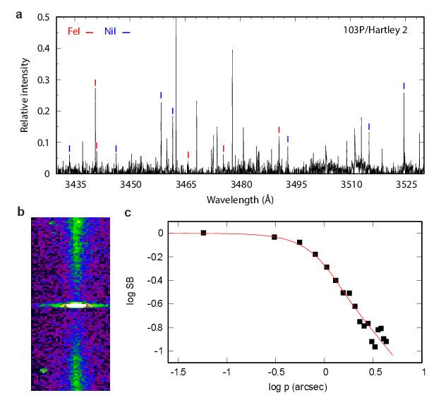
8Figure 1: Example of FeI and NiI lines in comet 103P/Hartley 2. a, Selected spectral region
showing many FeI and NiI lines in the spectrum of the Jupiter family comet 103P/Hartley 2 obtained
at the ESO VLT in April 2004 at 0.17 au from Earth. b, 2-dimensional spectrum of the FeI 3719 Å
line. Wavelengths are along the vertical axis and cover a range of 3 Å. The spatial dimension
(horizontal axis) extends over the entire length of the 10" slit (1230 km at the distance of the comet).
The vertical trace represents the solar spectrum reflected by the dust and shows the deep
photospheric absorption of the FeI 3719 line. c, The spatial profile of the same line plotted as a
function of the projected nucleocentric distance p agrees well with a 1/p distribution of the surface
brightness (SB) and a 1.35" blurring corresponding to the seeing and the tracking imperfections.
The NiI lines display the same kind of profile.
1Figure 2: Ni/Fe abundance ratios from the multilevel model versus heliocentric distance. The
best spectra have been selected and the great comet C/1965 S1 (Ikeya-Seki) has been added as
number 35. The vertical dashed-dotted line indicates the solar value and the dotted lines represent
the sample average and standard deviation. Different colors are used according to the dynamical
class34: Jupiter family comets in red and Halley family comets in pink correspond to ecliptic comets
with short periods (< 200 years), external comets in blue have a semi-major axis a < 10000 au and
new comets in black come directly come from the Oort cloud (a > 10000 au).
2Extended Data Table 1. Comets observing circumstances with UVES at ESO VLT. In several
cases, N spectra have been averaged. r and ∆ are the heliocentric and geocentric distances in au
and the dotted symbols are the corresponding velocities in km/s. The offset d from the nucleus, the
slit width w and the slit height h are given in arc seconds. Type refers to their dynamical class as
defined by34: JFC (Jupiter Family) and HFC (Halley Family) correspond to ecliptic comets with short
periods (< 200 years), EXT corresponds to external comets with semi-major axis a < 10000 au and
NEW corresponds to external comets which directly come from the Oort cloud (a > 10000 au).
3Extended Data Table 2. Ni/Fe abundance ratios from the 3-level and the multilevel models. T
is the excitation temperature used for both FeI and NiI, and nlines the number of FeI and NiI lines
considered in the analysis. The column densities N (atoms/cm2) and the production rates Q
(atoms/s) come from the multilevel model.
4Extended Data Table 3. Production rates of molecules and dust. Logarithm of the production
rates of the gaseous species OH, CN, CO 2+ (molecules/s), and, as a proxy of the dust production
rate, the Afρ parameter35, to which it is proportional for a 1/p brightness profile. Afρ is derived from
the dust continuum intensity around the CN band and is corrected for the phase effect, the seeing
and the slit geometry. The production rates of OH, CN and CO 2+ were derived from a Haser model.
For the OH and the CN bands, we used, respectively, the data from 36,37 for the A2Σ+ − X2Π (0,0)
band near 3090 Å and the B 2Σ+ − X2Σ+ (0,0) band near 3880 Å. For the CO 2+ A2Π −X2Π (0,0) band
near 3500 Å we assumed a simple Haser profile with one component, CO 2 being the parent. The
time scale and fluorescence efficiency are taken from 38,39. The profile distribution was integrated
over the area of the slit of the spectrograph and compared to the observed flux of the bands to yield
the production rate.
5Extended Data Fig. 1. Examples of UVES comet spectra. Comet spectra obtained with the
UVES spectrograph at ESO VLT, showing many Fe i and Ni i lines in the selected wavelength
region (3,425–3,530 Å). a, Spectrum of the water-poor and CO-rich long-period comet C/2016 R2
(PanSTARRS) at 3 au. b, Spectrum of the Jupiter-family comet 88P/Howell at 1.4 au. c, Spectrum
of the new comet C/2002 T7 (LINEAR) at 0.68 au, with lines from the OH(1-2) band. d, Spectrum of
the long-period comet C/2020 X5 (Kudo−Fujikawa). Fe i and Ni i lines are indicated by red and blue
marks, respectively.
6Extended Data Fig. 2. Comparisons of Fe I, Ni I and dust production rates. a-d, The
production rates of FeI and NiI are compared to Afρ which is the product of the reflectivity of the
grains, their filling factor and the radius of the coma (used as a proxy to the dust production rate)
and to the production rates of OH, CN and CO 2+ as determined from our spectra. e-f, The
production rates of FeI and NiI are compared to the production rates of H 2O and CO measured by
various authors in comets 8P, 9P, 21P, 73P, 103P, C/2000 WM1, C/2001 Q4, C/2002 T7,
C/2009 P1, C/2012 F6 and C/2016 R2 at about the same epochs as our observations 40–51. The
various cometary types are color coded according to their dynamical classification (see Extended
Data Table 1). The OH and H2O values relative to comet C/2016 R2 are upper limits. The Pearson’s
correlation coefficients calculated without (and with) the C/2016 R2 data are ρ OH = 0.844 (0.531),
ρAfρ = 0.644 (0.616), ρCN = 0.892 (0.518), ρCO2+ = 0.755 (0.804), ρH2O = 0.849 (0.627) and ρ CO = 0.752
7(0.770).
Extended Data Fig. 3. Iron and nickel carbonyl sublimation properties. a, The sublimation
rates (Z in molecules cm−2 s−1) of Fe and Ni carbonyls as a function of temperature, compared to
those of the main ices in comets. The carbonyl rates are intermediate between those of H 2O and
CO2. b, The sublimation rate ratio Ni(CO)4 over Fe(CO)5 shows that the sublimation rate of Ni(CO) 4
is significantly higher than the one of Fe(CO) 5. These quantities were computed as follows. As 52,53,
we estimate the condensation or sublimation temperature Ts of these compounds by solving the
equation fx n k Ts = Pv,x(Ts) where fx is the relative abundance of species x, n the number density of
the gas, k the Boltzmann constant, and Pv,x the vapor pressure given by the relation log Pv,x(T ) =
−A/T + B. The constants A and B for Fe(CO)5 and Ni(CO)4 are obtained from54,55, that is A = 2097 K
and B = 11.62 for Fe(CO)5, A = 1534 K and B = 10.87 for Ni(CO)4, with Pv,x in dyn cm−2. We consider
relative abundances fx between 10−3 and 10−5 × fx(H2O), for both Fe(CO)5 and Ni(CO)4, and we
adopt n = 1013 cm−3 as53. The resulting sublimation temperatures of the iron and nickel carbonyls
(respectively 97-108 K and 74-82 K, depending on fx) are intermediate between the sublimation
temperatures of H2O and CO2 (152 K and 72 K), while CO sublimates at 25 K 53. The sublimation
rate (in molecules cm−2s−1) from the surface of a pure ice into vacuum can be expressed as 56: Zx(T)
= Pv,x(T) (2πmxkT)−1/2 where T is the ice temperature and mx the mass of the species x.
End Notes
Supplementary Information is available for this paper.
Data availability statement
The datasets analyzed during the current study are available at the ESO Science Archive Facility at
http://archive.eso.org/eso/eso_archive_main.html, under programmes 073.C-0525, 075.C- 0355(A),
080.C-0615, 086.C-0958, 087.C-0929, 270.C-5043, 274.C-5015, 2100.C-5035(A), 280.C-5053
and 2101.C-5051. Correspondence and requests for materials should be addressed to J. Manfroid.
Email and orcid :
J. Manfroid jmanfroid@gmail.com 0000-0002-6930-2205
8Hutsemékers d.hutsemekers@uliege.be
Jehin ejehin@uliege.be 0000-0001-8923-488X
Reprints and permissions information is available at www.nature.com/reprints
Author contribution
JM analyzed the spectra and the coma profiles and wrote the main text. DH contributed to the
proposals and observations, reduced and calibrated the spectra, built the fluorescence model,
computed the carbonyl sublimation properties, and wrote the supplementary information. EJ lead
the UVES proposals and made most of the observations. All authors contributed to the discussion
and the final text.
Acknowledgements
We thank Dr. P. van Hoof for useful discussions on the iron atomic data and their uncertainties. We
thank R. Hewins and Prof. R. Warin for discussions about various Fe and Ni rich compounds in
meteorites. We thank C. Arpigny, D. Bockelée-Morvan, A. Decock, C. Opitom, H. Rauer, P.
Rousselot, and B. Yang for leading some UVES proposals, and the ESO staff for service mode
observations. JM, DH, and EJ are honorary Research Director, Research Director and Senior
Research Associate at the F.R.S-FNRS, respectively.
Competing interests. The authors declare no competing interests.
9Supplementary information
Iron and nickel atoms in comet atmospheres
J. Manfroid, D. Hutsemékers, and E. Jehin
STAR Institute, University of Liège
Allée du 6 Août 19c, B-4000 Liège, Belgium
Contents
1 FeI and NiI fluorescence models and abundance measurements 1
1.1 Method and results . . . . . . . . . . . . . . . . . . . . . . . . . . . . . . . . . . . . . . . . . 1
1.2 Three-level atom . . . . . . . . . . . . . . . . . . . . . . . . . . . . . . . . . . . . . . . . . . 3
1.3 Multilevel atom . . . . . . . . . . . . . . . . . . . . . . . . . . . . . . . . . . . . . . . . . . . 4
1.4 Multilevel versus three-level model . . . . . . . . . . . . . . . . . . . . . . . . . . . . . . . . . 5
1.5 Tests, possible improvements, and robustness of the results . . . . . . . . . . . . . . . . . . . . 5
1.6 Figures . . . . . . . . . . . . . . . . . . . . . . . . . . . . . . . . . . . . . . . . . . . . . . . 6
1 FeI and NiI fluorescence models and abundance measurements
1.1 Method and results
Preston [1] found that the intensity of the FeI and NiI emission lines observed in comet C/1965 S1 (Ikeya-Seki)
at 0.14 au from the Sun can be related to the energy of the upper level of the transitions through a Boltzmann
distribution, and that these lines are likely formed by resonance fluorescence. A simple “curve-of-growth” analy-
sis then provided the excitation temperature of the lines and allowed the determination of the NiI/FeI abundance
ratio. In Sect. 1.2, we explicitly reformulate the resonance fluorescence model [2, 3] considering a 3-level atom
and assuming that the solar radiation can be represented by a diluted blackbody. For each comet the excita-
tion temperature is empirically determined following Eq. 14 using the observed FeI emission line intensities and
atomic data from the Atomic Line List v2.05 [4]. Fig. S1 illustrates the empirical method used to estimate the
excitation temperature for two representative comets. For NiI, the smaller range of upper energy levels precludes
an accurate determination of the excitation temperature but, given the similar atomic level structure of FeI and
NiI, we assume T (NiI) = T (FeI) as in [1–3]. Suspected blends1 are not considered and a few recurrent outliers
are discarded from the analysis, in particular a few FeI lines with lower energy levels higher than 2 eV, and the
two NiI lines with the smallest log(g f ). In two comets, the number of observed FeI lines is too small to derive the
temperature and we adopt T = 4000±1000 K, which is representative of the sample. The NiI/FeI abundance ratio
is finally obtained from Eq. 15 with log UNi /UFe = 0.06 ± 0.02 computed for the temperature range 3500-5000 K.
Errors on the mean abundance ratio account for the dispersion of the C values (fixed to 0.3 dex when the line
number is smaller than 3) and the range of acceptable temperatures. The NiI/FeI abundance ratios computed with
the 3-level model are given in Extended Data Table 22 . The metallic lines found in comet Ikeya-Seki were simi-
larly analyzed3 , considering only the FeI and NiI lines that are also detected in our spectra to avoid any bias. The
1
Examples are the bright FeI 3859.91 Å and 3856.37 Å lines which are blended with the generally much stronger CN R4 3859.95 Å
and R9 3856.40 Å lines, respectively, as well as the NiI 3458.46 Å line which is often overwhelmed by some underlying line.
2
Abundance ratios show little dependence on the temperature as far as the same excitation temperature is used for both FeI and NiI.
Column densities, on the other hand, strongly depend on the adopted temperature and are therefore not reported in the Table.
3
The line intensities are taken from [1]. This paper provides equivalent widths in units of the sky spectrum intensity and argues that
the sky spectrum is mostly independent of wavelength (“white”) so that the equivalent widths can be used as intensities with an error that
can be as high as 30%.
1NiI/FeI abundance ratio we derive for comet Ikeya-Seki is in excellent agreement with previous studies [1–3].
Although the 3-level model seems to provide a reasonably good interpretation of the FeI and NiI emission spec-
trum, it is based on approximations that need to be tested, in particular the assumption of identical excitation
temperatures for the FeI and NiI lines, and the use of a blackbody for the solar radiation (strong metallic lines
in absorption are known to sprinkle the solar spectrum). We therefore built a multilevel atomic model where the
true solar spectrum is taken into account. The model is detailed in Sect. 1.3. Input atomic data are extracted from
the Atomic Line List v2.05 [4]. For FeI, we consider transitions with lower levels in the energy range 0-20000
cm−1 , upper levels in the energy range 0-40000 cm−1 , and line strengths with Aki > 103 s−1 . These constraints
ensure that all useful observed transitions are included, while keeping the number of levels reasonably small.
This results in 427 transitions with wavelengths between 2500 Å and 13000 Å for 85 energy levels including
the ground level. For NiI, we use the same constraints with upper levels in the energy range 0-50000 cm−1 . For
the solar spectrum, we use the calibrated high-resolution spectrum of [5]. The spectral range is 2960-13000 Å,
with a resolving power between 350000 (UV) and 500000 (IR). For the spectral range 2000-2960 Å, we use the
calibrated solar spectrum of [6] which has a lower spectral resolution of 0.1 Å.
In Fig. S2, the FeI lines intensities computed with the model are compared to the measured intensities in four
comets. The computed spectra reproduce reasonably well the observed spectra, although for some lines, differ-
ences can be significant, possibly due to unrecognized blends, measurement errors, or uncertainties of the atomic
data which can be large [7]. For comets 103P and especially C/2016 R2, the dispersion of the intensity ratios
is higher than for Ikeya-Seki, and some bright lines not well reproduced. Differences between Ikeya-Seki and
other comets with respect to the model could be, at least in part, attributed to the strong difference in heliocentric
velocities, +110 km s−1 for Ikeya-Seki versus +3.5, -5.6 and +25.6 km s−1 for 103P, C/2016 R2 and C/2002 T7,
respectively. The solar spectrum shows deep FeI and NiI absorption lines so that the radiation reaching the comet
is strongly dimmed at low heliocentric velocities (Fig. S3). For high enough Doppler velocities, the radiation
reaching the comet is expected to be more homogeneous for the different metallic lines, and closer to a black-
body. This emphasizes the importance of the comet heliocentric velocity as the cometary FeI and NiI transitions
can sample very different portions of the solar spectrum depending on the Doppler shift.
In Fig. S4, the Iobs /Imod ratios (Eq. 20) are shown on a logarithmic scale for both the FeI and NiI lines. While
the dispersion of log(Iobs /Imod ) can be high, significant differences between the relative mean FeI and NiI column
densities are clearly seen between these comets. The column densities of FeI and NiI are given in Extended Data
Table 2, as well as the derived NiI/FeI abundance ratios. The errors of the mean column densities are estimated
from the standard deviation of the logarithmic column densities computed from individual lines (fixed to 0.3 dex
when the line number is smaller than 3), divided by the square root of the number of lines. Errors thus include
measurement errors and uncertainties of the atomic data.
In Sect. 1.4, we compare the results from the two models. The fact that the excitation temperatures estimated
with the 3-level model are systematically lower than the Sun color temperature can be explained, at least in part,
by the presence of strong absorption lines in the true solar spectrum. The NiI/FeI abundance ratios computed
with the 3-level model nicely correlate with those ones derived from the multilevel model although they show
a systematic shift of ∼0.2 dex (Fig. S6). The difference between the two models appears mainly due a proper
account of the solar radiation spectrum in the multilevel model rather than to the number of levels used in the
computation.
Tests and possible improvements are discussed in Sect. 1.5. They essentially show that the measured abundance
ratios are robust. In particular, increasing the number of atomic transitions and levels does not improve the
derived quantities. To improve the fits, better intensity measurements (deblending) and more accurate atomic
data would be needed. Finally one should keep in mind that the fit of individual lines may also be affected by
the lower spectral resolution of the solar spectrum at wavelengths smaller than 2960 Å. Several transitions from
the ground level do occur in that wavelength range for which the incoming solar flux might not be accurately
estimated, especially at low heliocentric velocities.
21.2 Three-level atom
In addition to the ground level, FeI and NiI show a few metastable lower levels and upper levels of opposite parity.
Observed transitions occur between the two sets of levels [2, 3, 8]. We then consider a 3-level atom, excited by
resonance fluorescence. Statistical equilibrium for the ground and the lower levels writes
nl (Alg + Blg Jlg ) + nu (Aug + Bug Jug ) = ng (Bgl Jgl + Bgu Jgu ) , (1)
ng (Bgl Jgl ) + nu (Aul + Bul Jul ) = nl (Alg + Blg Jlg + Blu Jlu ) , (2)
where ng , nl , and nu are the volume density of atoms in the ground, lower,
R and upper levels, respectively. A, B are
the Einstein coefficientsRand J the mean intensity of the radiation. Ji j = J(ν) φ(ν) dν over the natural line profile
that is Ji j ' J(νi j ) with φ(ν) dν = 1. Since the lower level is metastable, transitions g ↔ l can be neglected and
these relations simplify to
nu Bgu Jgu
= , (3)
ng (Aug + Bug Jug )
nu Blu Jlu
= . (4)
nl (Aul + Bul Jul )
The Einstein coefficients are related by Aui /Bui = 2hνui3 /c2 and g B = g B for i = g, l. Assuming J = W B
i iu u ui ν ν
where Bν (T ) = (2hν /c )/(e
3 2 hν/kT − 1) represents the solar blackbody radiation at frequency ν and temperature T ,
and W the dilution factor s
1 R2 1 R2
W = (1 − 1 − 2 ) ' , (5)
2 r 4 r2
R denoting the solar radius and r the comet heliocentric distance, we derive
nu gu 1
= . (6)
ni gi 1 + (ehνiu /kT − 1)/W
Since W
1 and assuming hν
kT (Wien approximation) we can finally write
χu
nu /ng = W (gu /gg ) 10−θ , (7)
−θ (χu −χl )
nu /nl = W (gu /gl ) 10 , (8)
−θ χl
nl /ng = (gl /gg ) 10 , (9)
where θ = 5040 K / T and χu (χl ) is the energy of the upper (lower) level in eV. If n is the volume density of the
χ
atom in all states, nl /n = gl 10−θ l /U(T ) where U(T ) is the partition function, so that we have
χu
nu gu 10−θ
=W . (10)
n U(T )
Due to the dilution of the exciting radiation, the upper levels are weakly populated with respect to the lower ones
χ
and U(T ) ' gg + l gl 10−θ l .
P
The intensity integrated over the line of sight of the radiation emitted in the transition u → i with i = g, l, is given
by Z
1
Iν = jν ds where jν = nu Aui hνui φ(ν) . (11)
4π
Using the oscillator strength
mc3 gu
fiu = 2 g
Aui (12)
8π2 e2 νui i
3we write χ
8π2 e2 h gi fiu 10−θ u
Iν = N W φ(ν) (13)
4πm λ3ui U(T )
where N =
R
n ds is the column density. This relation can be written in the form
Iλ3
log = −θ χu + C (14)
gf
that allows the Rempirical determination of θ by plotting log(Iλ3 /g f ) against χu for observed spectral lines.
I = Iν dν = Iλ dλ is the intensity (surface brightness) integrated over the observed line profile. Relative
R
abundances of two atoms 1 and 2 can then be obtained using
N1 U1
log = (C1 − C2 ) + log , (15)
N2 U2
where the constants C are computed from Eq. 14 for each observed line of a given atom using the estimated value
of θ, and then averaged over all observed lines.
1.3 Multilevel atom
We consider m energy levels. Statistical equilibrium for level i reads
m
X m
X
n j Q ji = ni Qi j (16)
j=1 j=1
j,i j,i
where Qi j = Bi j Ji j for i < j, Qi j = Ai j + Bi j Ji j and Ai j = Bi j (2hνi3j /c2 ) for i > j, and gi Bi j = g j B ji . By defining
Qii = − mj=1 Qi j and n0j = n j /n1 , we finally have for level i
P
j,i
m
X
n0j Q ji = −Q1i , (17)
j=2
that is a system of m linear equations with m − 1 unknowns. By dropping the i = 1 redundant equation, and
denoting αi j = Q j+1,i+1 , βi = Q1,i+1 and x j = n0j+1 for i, j = 1, m − 1, we write the matrix equation
α11 α12 ··· αm−1,1 x1 β1
α α ··· αm−1,2 x2 β
21 22 2
.. .. .. .. .. = ..
(18)
. . . . . .
αm−1,1 αm−1,2 · · · αm−1,m−1 βm−1
xm−1
that we solve with the Gauss-Jordan elimination method [9] to derive the atomic level population ratios n0j . With
n j /n = n0j /(1 + m 0
P
k=2 nk )), line intensities are finally obtained for each transition j → i:
h n0j
I ji = N 0 A ji ν ji . (19)
4π 1 + m
P
k=2 nk
The high-resolution solar spectral irradiance Fλ given in [5] and [6] at 1 au is converted into mean intensity in
the coma using Ji j = J(νi j ) = (4πc)−1 Fλ λ2i j r−2 where r is in au.
Denoting Imod (= I ji for N = 1 cm−2 ) and Iobs the computed and observed line intensities integrated over the
4observed line profile, respectively, the logarithmic column density is derived using
Iobs
log N = log . (20)
Imod
For a set of observed lines, log N is averaged over all lines, and the abundance ratio of atoms 1 and 2 given by the
ratio of their mean column densities.
1.4 Multilevel versus three-level model
The comparison of the two models (Fig. S5) shows that the 3-level atomic populations reproduce fairly well the
populations computed with the multilevel model, provided that the blackbody temperature adopted in the 3-level
model is significantly lower than the Sun color temperature. We also estimated the excitation temperature using in
Eq. 14 the FeI line intensities generated by the multilevel model. For cometary heliocentric velocities of 5 km s−1
and 100 km s−1 , we derive T ' 4000 K and T ' 4500 K, respectively. The fact that the excitation temperature is
smaller than the color temperature of the Sun (∼ 5800 K) is thus mostly due to the fact that the flux from the solar
spectrum is fainter than a blackbody due to the strong absorption lines, in particular when the Doppler velocity is
close to zero (Fig. S3).
As shown in Fig. S6, there is an overall agreement between the NiI/FeI abundances estimated with the two
models but also a clear systematic offset: the abundance ratios derived with the 3-level model are about 0.2 dex
larger than the abundance ratios derived with the multilevel model. A better agreement is obtained by assuming
T (NiI) = T (FeI)+180 K in the 3-level model.
1.5 Tests, possible improvements, and robustness of the results
We performed several tests modifying the constraints on the selected energy levels and minimum transition
strength, and considering up to 668 energy levels and 3435 transitions for FeI. No significant changes of the
level populations or line intensities were observed in the spectral range of interest, i.e., 3300-4500 Å. We also
considered alternative atomic data sets, in particular from [10], and found no significant differences in the model
results.
The effect of collisions was also investigated, with the aim to better fit the observed line intensities. A collisional
χ χ
term Ci j was added to the Qi j defined in Sect. 1.3, with Ci j /C ji = (g j /gi ) × 10 θ( i − j ) . An approximate formula
for estimating collisions with electrons is given by [11]. Given the low density and low temperature prevailing in
cometary comae, collisions with electrons are negligible. Collisions with atoms or molecules might be considered
but, as far as we know, no estimates are available for cometary atmospheres. We thus parametrized collisional
de-excitation as C ji = [θ(χ j − χi )]δ where and δ are free parameters. Tests done by varying these parameters
indicate that introducing collisions does not improve the model and most often gives poorer fits.
We also considered extinction by dust in the inner coma using the standard CCM extinction curve [12]. Both the
incoming solar radiation and the outward emitted lines were assumed to be reddened. For C/2016 R2, assuming
AV ' 1.5 (which is a reasonable value for the extinction in the inner coma [13]) makes the dispersion in Fig. S4
slightly smaller, while keeping the abundance ratio unchanged.
51.6 Figures
Figure S1: Empirical determination of the excitation temperature. FeI emission lines observed in two rep-
resentative comets are used. Outliers not considered in the fit are shown in green. For C/2016 R2 (and only for
that comet) additional outliers were discarded through an iterative fit. Error bars account for the errors on the
measured intensities and an uncertainty of log(g f ) assumed to be 0.2 dex.
6Figure S2: Comparison of the observed and modeled spectra. A portion of the FeI spectrum is shown for four
representative comets. Observed line intensities are in black; computed line intensities are in red and shifted by
0.7 Å for visibility. Intensities are in arbitrary units. The intensities from the model have been scaled using the
ratio Iobs /Imod averaged over all observed lines.
7Figure S3: Sample of the Kurucz solar spectrum. The red crosses indicate the value of the solar flux involved
in three cometary FeI transitions. The solid blue line represents a blackbody spectrum with T = 5800 K, and the
dashed blue line a blackbody spectrum with T = 4000 K. Cometary heliocentric velocities are equal to 0 km s−1
(left) and +20 km s−1 (right). The solar flux is given in arbitrary units.
Figure S4: Abundance ratio determination. The ratio log(Iobs /Imod ) = log N measured for the FeI (red) and
NiI (blue) lines in four comets. The ratios have been shifted on the y-axis so that the mean of log(Iobs /Imod ) is
zero for FeI. The few outliers have been discarded. The difference of the means computed for all FeI and NiI
lines gives the log(NiI/FeI) abundance ratio.
8Figure S5: Comparison of upper level populations. The level populations are computed for FeI with the
3-level (3L) and multilevel (ML) atomic models. Left: Black squares represent 3-level populations computed
with a blackbody temperature of 5800 K (the color temperature of the Sun) while red squares represent 3-level
populations computed with a temperature of 4400 K in better agreement with the multilevel populations computed
with the Kurucz solar spectrum. Right: Same as in the previous figure, but with the solar spectrum shifted by
20 km s−1 . The red squares represent 3-level populations computed with a temperature of 5000 K.
Figure S6: Abundances from the two models. Comparison of log(NiI/FeI) abundances derived with the mul-
tilevel (ML) model and the 3-level (3L) model for the comets of our sample. Left: Assuming T (NiI) = T (FeI).
Right: With T (NiI) = T (FeI)+180 K.
9References
1 G. W. Preston, “The spectrum of Ikeya-Seki (1965f)”, ApJ 147, 718–742 (1967).
2 C.Arpigny, “On the nature of comets.”, in Proceedings of the robert a. welch foundation conferences on
chemical research xxi, cosmochemistry, edited by W. Mulligan (1978), p. 9.
3 C.Arpigny, “Relative abundances of the heavy elements in comet Ikeya-Seki /1965 VIII/”, in Liege interna-
tional astrophysical colloquia, Vol. 22, edited by A. Boury, N. Grevesse, and L. Remy-Battiau, Liege Interna-
tional Astrophysical Colloquia (Jan. 1979), pp. 189–197.
4 P. A. M. van Hoof, “Recent Development of the Atomic Line List”, Galaxies 6, 63 (2018).
5 R. L. Kurucz, I. Furenlid, J. Brault, and L. Testerman, Solar flux atlas from 296 to 1300 nm (1984).
6 L.
A. Hall and G. P. Anderson, “High-resolution solar spectrum between 2000 and 3100 Å.”, J. Geophys. Res.
96, 12, 927–12, 931 (1991).
7 J.
R. Fuhr and W. L. Wiese, “A Critical Compilation of Atomic Transition Probabilities for Neutral and Singly
Ionized Iron”, Journal of Physical and Chemical Reference Data 35, 1669–1809 (2006).
8 C. E. Moore, Partial Grotriam diagrams of astrophysical interest (1968).
9 W. H. Press, S. A. Teukolsky, W. T. Vetterling, and B. P. Flannery, Numerical recipes in FORTRAN. The art of
scientific computing (1992).
10 G.
Nave, S. Johansson, R. C. M. Learner, A. P. Thorne, and J. W. Brault, “A New Multiplet Table for Fe i”,
ApJS 94, 221 (1994).
11 H. van Regemorter, “Rate of Collisional Excitation in Stellar Atmospheres.”, ApJ 136, 906 (1962).
12 J.
A. Cardelli, G. C. Clayton, and J. S. Mathis, “The Relationship between Infrared, Optical, and Ultraviolet
Extinction”, ApJ 345, 245 (1989).
13 P. Lacerda and D. Jewitt, “Extinction in the Coma of Comet 17P/Holmes”, ApJ 760, L2, L2 (2012).
10You can also read