ISSI Wg Microwave Scatterometers

Royal Netherlands
 Meteorological Institute
 Ministry of Infrastructure and Waterworks

 ISSI Wg
 Microwave
 Scatterometers
 Ad.Stoffelen@knmi.nl
ASCAT cone metrics
 EUMETSAT OSI SAF: L2 data services
 EUMETSAT NWP SAF: software
 EU Copernicus Marine Core Services: L3/4

 Alphen NB, 18 May 2021

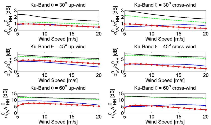
Ku

 C Ku

 Ku

Ku C

 Franco Fois, PhD thesis, 2015

Satellite µw scatterometers
 Ground-based transponders are inaccurate for quality monitoring, but provide ball-
 park calibration for ASCAT
 The rain forest has a daily cycle of about 15% in µw backscatter; it may be used for
 stability monitoring at given LTAN
 Land targets are affected by moisture events (dew, rain)
 Ice/snow targets may be stable for months, years or decades, but will be affected by
 T>0 / rain (climate change)
 No absolute calibration, but
  Very stable instruments within 0.1 dB (2%)
  Cone metrics provides order 0.02 dB calibration for ASCAT (0.02 m/s)
  Excellent relative calibration between instruments and over time
  Non sun-synchronous satellite references for intercalibration
  Excellent and consistent GMFs at used wavelengths, polarizations and angles
  Many close C- and Ku-band collocations, allowing improved GMFs and consistency
  Reasonable control on ancillary parameters: SST, stability, waves, rain, . . .
  Well-known and controlled in situ and NWP references (except for extremes)
  Generic C- and Ku-band processors
 Use ASCAT 2013 as calibration reference?

Satellite µw scatterometers
 Bragg scattering interference of microwaves and ocean waves
 Hydrodynamic ocean short-wave modulation, choppy wave model
 Wave-wind interaction, wave boundary layer (scatterometers see no long waves so far)
 The short wave spectrum is dominated by breaking waves and their dissipation for
 modal and higher winds
 Crucial to describe the short wave spectrum, but rather complex
 Use satellite data

 Wave shadowing and
 interference at grazing
 incidences

 Specular reflection
 dominates
 at smaller incidence
 angles
 (geometric optics)

 Scattering spilling breakers

Uncertainty
 Users are interested in stability and consistency of L2 geophysical products,
 e.g., detect 0.1 m/s trends over 10 years
  Cone metrics provides order 0.02 dB calibration for ASCAT (0.02 m/s)
 Cone spread over ocean to provide ocean spatial variability, which is found
 equal to wind variability (wind downbursts, turbulence, convection)
 Related to Kp too (Kp is the σ0 SD)
 Can be segregated into geophysical and instrument contributions
 Wind retrieval quality is in stress-equivalent wind, correcting for air stability
 and mass density effects
 Scatterometer wind retrievals are very consistent after intercalibration of
 backscatter values and GMFs
 Physically-based models are useful to describe/understand behaviour at
 different wavelengths and polarizations, but fed by empirical satellite data
 characterization to improve accuracy
  Wavelength dependency
  Wind azimuth and speed dependency
  Polarization/incidence dependency

 Franco Fois, PhD thesis, 2015

Scattering models

 SPM Small Perturbation Method
 KA Kirchhof Approximation
 HF High Frequency, small wavelength
 GO Geometric Optics (longer sea waves)
 SSA Small Slope Approximation
 WCA Weighted Curvature Approximation

Franco Fois, PhD thesis, 2015

Franco Fois
 High Frequency: GO and Kirchhoff
 Low Frequency: SPM
 Unified models (GO and SPM), multiple scattering: SSA2
 SSA2 best fits GMF data at C, X and Ku bands
 Steep breaking waves point of concern
 Foam, small co-pol effect and large VH effect for high winds
 Mouche et al. find Tb and VH both linear with extreme winds
 Non-linear hydrodynamic coupling between long and short waves

GMF:
σo = A0 + A1 cos φ + A2 cos 2φ

σo = B0 [1+ B1 cos φ + B2 cos 2φ]0.625 adds higher harmonic terms to fit cone
Stoffelen and Anderson (1997)

 Franco Fois, PhD thesis, 2015

Ku-band vs θ
 SASS/NSCAT-4 Ku VV and DV1.25/SSA2
 θ dependency match
× Not for Kudryavtsev
× HH DV1.25/SSA2/Kudry θ dependency
 too steep

C-band vs θ
 ** * CMOD7
 CMOD VV and DV1.25/SSA2 *
 θ dependency match @ 10 m/s * *
× Not for Kudry *
× Particularly not at lower speeds
 for DV1.25

C-band VV ASAR θ=39.5o
 __ upwind
 ASAR not calibrated w.r.t. ASCAT - - cross
 Radars need calibrated noise
 subtraction (noise floor) and linear
 calibration (dB off-set), e.g., Belmonte CMOD5n
 et al. (2017) on cone metrics SSA2-Hwang
 ASCAT calibration is checked with SSA2-Elfouhaily
 transponders; remaining absolute
 uncertainty ~0.2 dB
 Relative uncertainty CMOD7/CMOD5n
 typically 0.1 dB
 ASAR noise subtraction?

 C-band VV-HH (θ=45o) = 5.4 dB
 (Thompson)

 CMOD steeper as function of speed

 Franco Fois, PhD thesis, 2015

C-band HH ASAR θ=39.5o
 __ upwind
 ASAR not calibrated w.r.t. ASCAT - - cross
 Radars need calibrated noise
 subtraction (noise floor) and linear
 calibration (dB off-set), e.g., Belmonte CMOD5n
 et al. (2017) on cone metrics SSA2-Hwang
 ASCAT calibration is checked with SSA2-Elfouhaily
 transponders; remaining absolute
 uncertainty ~0.2 dB
 Relative uncertainty CMOD7/CMOD5n
 typically 0.1 dB
 ASAR noise subtraction?

 C-band VV-HH (θ=45o) = 5.4 dB
 (Thompson)

 CMOD steeper as function of speed

C VV ASAR θ=39-41o C HH ASAR θ=39-41o

 __ SSA2 10 m/s
 - - SSA2 5 m/s

 C-band
 CMOD VV and DV1.25
 φ modulation match
 HH DV1.25 matches
 up/downwind Ku
 shape
× Kudry

Zheng et al., Remote Sens. 2018, 10(7), 1084; https://doi.org/10.3390/rs10071084

 VV HH

 C-band
 CMOD VV and DV1.25
 φ modulation match
 HH DV1.25 matches
 up/downwind C/Ku
 shape
× Kudry

Breaking contribution
 Steep breaking waves needed for HH at high θ
 Non-Bragg scattering spilling breaking waves
 Reul et al., 2008
 Improves polarization ratio

 WCA-Elfouhaily WCA-Kudryavtsev WCA-Hw+breaking NSCAT2 GMF
 Franco Fois, PhD thesis, 2015

From GMFs to physics

 Reul et al., 2008

 Hwang & Fois (2015)
 VV GMFs to approximate multifrequency Bragg, i.e., short wave spectrum
 HH and VH GMFs for refining scattering properties, Bragg, specular, non-Bragg
 scattering spilling breaking waves, foam, . . .

 Franco Fois, PhD thesis, 2015

Foam at extremes
 Tb and C-band VH NRCS
 both linear on dropsonde
 speed scale (Mouche et al.,
 2017)
 Foam phenomana is
 complex and linearity
 physically not plausible
 Inconsistent with moored
 buoy in-situ speed (U)
 scale from 15-25 m/s,
 which shows non-linear U [m/s]
 dependency (CHEFS)

L-band Aquarius

 VV HH VV HH VV HH

θ=29o

θ=38o

θ=46o

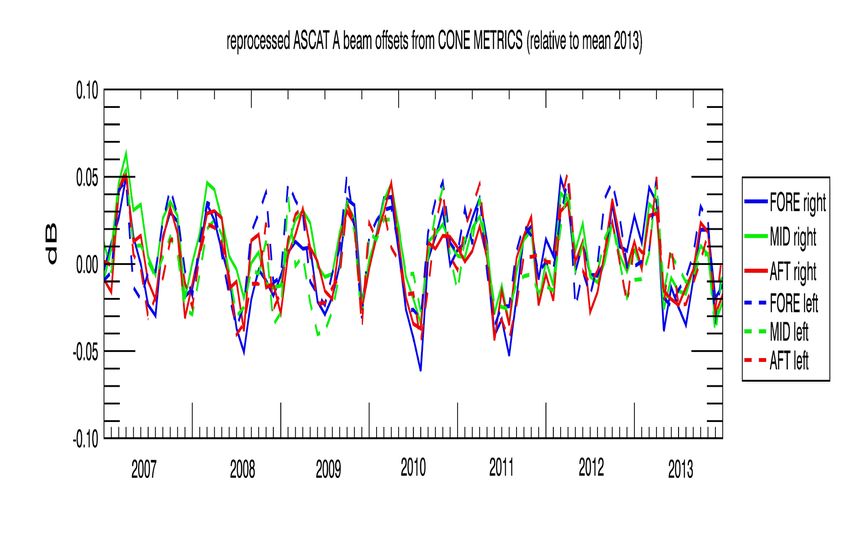
ASCAT is very stable
• ASCAT-A beams stay within a few hundreds of a dB (eq. to m/s)
• Cone position variation due to seasonal wind variability (reduced with u10s)
 Improve ASCAT attitude knowledge? (cf. Long, 1998)
 Asset for Ku-band scatterometer developments; radiometers
 Reference for NWP reanalyses
 Can method be applied for other scatterometers?

 Maria Belmonte et al., 2017

Stress-equivalent wind
 Radiometers/scatterometers measure ocean roughness
 Ocean roughness consists in small (cm) waves generated by air impact and
 subsequent wave breaking processes; depends on gravity, water mass density,
 surface tension s, and e.m. sea properties (assumed constant)
 Air-sea momentum exchange is described by τ = ρair u* u* , the stress vector; depends
 on air mass density ρair , friction velocity vector u*
 Surface layer winds (e.g., u10) depend on u* , atmospheric stability, surface
 roughness and the presence of ocean currents
 Equivalent neutral winds, u10N , depend only on u* , surface roughness and the
 presence of ocean currents and is currently used for backscatter geophysical model
 functions (GMFs)

 u10S = √ρair . u10N/√ρ0 is now used to be a better input for backscatter GMFs (stress-
 equivalent wind)
 This prevents regional biases against local wind references

 Jos de Kloe et al., 2017

Intercalibration and standardization
 Our premise is that for given wavelength, polarization and geometry, σ0
 should be identical in identical geophysical conditions and independent of
 instrument settings
 We develop generic L2 wind processing for calibrated instrument data
 Noise properties do however affect σ0 diagnostics, so we develop noise
 models too to better understand our retrievals and diagnostics
 KNMI is particularly interested to remove (σ0 –dependent) instrument
 biases as they interfere with Ku-band wind and SST dependencies
 (Stoffelen et al., 2017; Wang et al., 2017; Belmonte et al., 2017)
 Comparison of ScatSat with QSCAT, RSCAT and OSCAT behavior for given
 Geophysical Model Function GMF and NWP input to obtain consistency
 CFOSAT, HY-2 and WindRad scatterometers will follow

Rain & QC affect ocean calibration
 90% 9.4%

 RAIN RAIN

 RSCAT RSCAT
 ASCAT ASCAT
RSCAT

 ASCAT
 ASCAT

 0.3% 0.3%

 RAIN RAIN

 RSCAT RSCAT
 W. Lin et al., 2017 ASCAT
RSCAT

 ASCAT
IGARSS’15 ASCAT

0
 Δ RSCAT minus ASCAT
 Δ 0 RSCAT minus simulated by NSCAT4 GMF with ASCAT winds

Negative,
obs.HH is lower than VV
the ASCAT winds

 HH

 Large and Negative,
 obs.VV is much lower
 than the ASCAT winds
 Inner-Swath Cases, i.e., collocated HH&VV
 Basic dependencies similar to those in physically-based models
 Zhixiong Wang et al., 2017

ScatSat retrievals
  After correction for σ0 >= -19dB:
 σ0 (new) = σ0 (old) +
 [σ0(old)+19]*0.11

  QC not normalized
 VV only  Non-linear σ0 calibration !

 HH only HH + VV
 After Cal/Val some unexplained non-linear behaviour in Ku-band systems

 Anton Verhoef et al., 2017

Intercalibration
Can we make further improvements? Yes, we can:
 Pencil-beam scatterometers provide fixed combinations of polarization, incidence
 angle and azimuth angle at each WVC; these could be used for 4D “cone metrics” and
 provide a measure for long-term σ0 stability and consistency
 Ocean calibration needs development for new class of CFOSAT and WindRad rotating
 fan-beam scatterometers; NSCAT-ERS collocations may be used
 NWP ocean calibration procedures will provide first guidance for CFOSAT and WindRad
 Effects of rain, SST need to be further controlled in any Ku approach, be it “cone
 metrics” or NWP based
 A stable non-synchronous satellite instrument remains extremely useful for
 intercalibration and geophysical development, which latter is needed for improved
 error budgets for some calibration methods
 Error propagation in calibration methods and wind retrieval need to be better
 understood; “cone metrics” (MLE) provides measure of noise
 “cone metrics” will be used to improve GMFs to better describe measured σ0 PDF
 Improve understanding of in situ wind references to allow absolute wind calibration at
 high and extreme winds (CHEFS)

Inconsistencies in wind references

 Are dropsondes too high, or moored buoys and ECMWF too low at 15-25 m/s ?
 EUMETSAT CHEFS project addresses this; WL150 not suitable for calibration

 K.-H. Chou et al., 2013

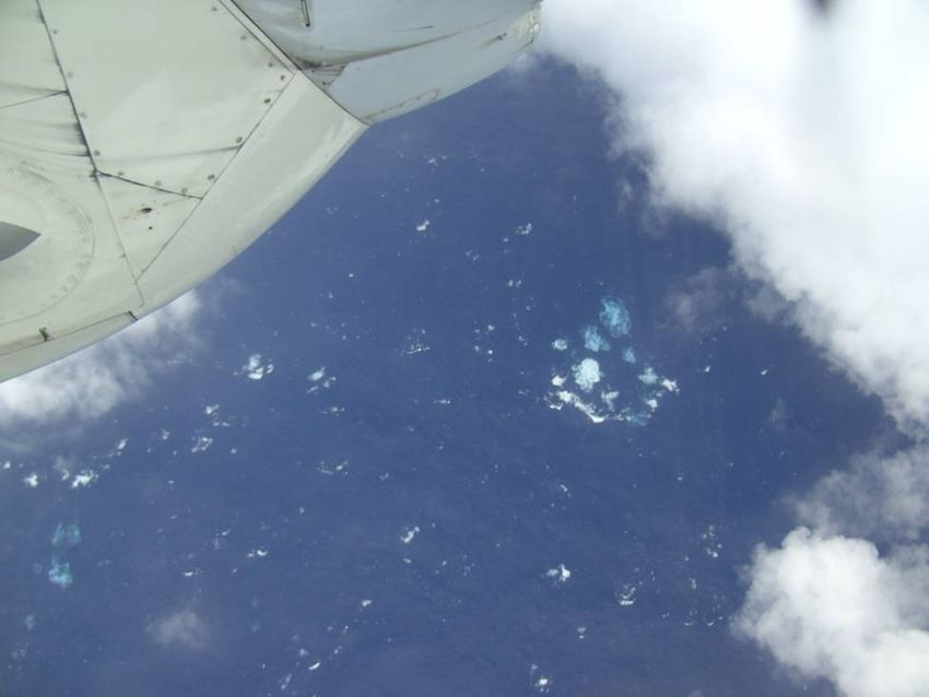
Maximum wind with sea view
SFMR: 85 knots (43 m/s; 157 km/hr )
@2.4 km: 125 knots (64 m/s; 232 km/hr)
Large foam patches near breaking wave fronts
No apparent saturation (uniformity)

Turbulent sea in the eye (with no wind!)

Global wind speed biases

 28

Model Wind Errors
 Typically 0.5 to 1 m/s in component bias and SD (10-20%) on model scales
 Underestimation of wind turning in NWP model: surface winds more aligned
 to geostrophic balance above than to pressure gradient below  stable
 model winds are more zonal with reduced meridional flows
 Sandu (ECMWF) reports that turbulent diffusion is too large (enlarged to
 reduce sub-grid mesoscale variability) which helps improve the
 representation of synoptic cyclone development at the expense of reducing
 the ageostrophic wind turning angle ...
 It is a problem that the ocean is forced in the wrong direction though

 Other processes poorly represented include 3D turbulence on scales below
 500 km and wide-spread wind downbursts in (tropical) moist convection
 (King et al., 2017)
 Atmospheric mesoscale variability stirs the ocean and enhances fluxes
 Adaptive bias correction needed for data assimilation and ocean forcing

Zonal, Meridional Errors
 ASCAT - ERAint
 
 ASCAT

 Systematic errors are larger than interannual variability

Zonal, Meridional Errors
 ERA5 has spatial error patterns similar to ERAint (only reduced in amplitude by ~20%)

 ERA5 - ASCAT

 Excess mean model zonal winds (blues at mid-latitudes and subtropics)
 Defective mean model meridional winds (reds at mid-lats and tropics)

Belmonte and Stoffelen, 2019

Transient Wind Errors

 u’ v’

 ERA5 - ASCAT
  Defective model wind variability overall:
 - Zonal (left) and meridional (right) at mid-to-high latitudes
 - Particularly meridional deficit along ITCZ
 - Locally enhanced along WBCs (ARC, ACC, GS, KE currents)

Belmonte and Stoffelen, 2019

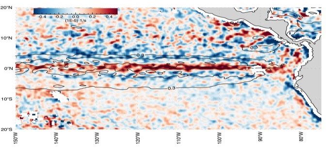
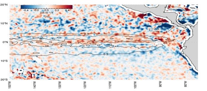
Effect of Globcurrent
Eastern Tropical Pacific

 Globcurrent accentuates
 SST effects in ASCAT
 winds that are missing
 in ECMWF winds
 Before
 Provides much better
 alignment of ECMWF
 discrepancies with
 branched SEC (N and S)
 to show positive curl
 error in between

 After
 Black contours are ocean velocities
 Mean wind speed Mean wind stress curl
 differences to ERA5 differences to ERA5
Belmonte and Stoffelen, 2019

Corrected ERA with ASCAT, OSCAT

 v

 -20 -15 -10 -5 0 5 10 15 20
Corrected wind component (v) 20130115 at 06 UTC with 1-day average of ASCAT-A, -B and ScatSat

 Trindade et al., 2019

Verification of ERA* with HSCAT
 ASCAT and ScatSat at 9:00-9:30 LTAN and HY2A SCAT at 6 am/6 pm LTAN
ASCAT and OSCAT at 9:00-9:30 LTAN and HY2A SCAT at 6 am/6 pm LTAN
 A = ASCAT-A
 B = ASCAT-B
 O = ScatSat

 ASC

 T ML T+ML

 DSC

 Statistics over 8-d periods
 Trindade et al., 2019

Model Corrections
①small
 Due to the persistence of the bias between model and scatterometer data it is possible to add
 scale information, i.e., include some of the physical processes that are missing or
 misrepresented in ERAi, and reduce the ERAi errors

②kept
 ERA* shows a significant increase in small-scale true wind variability, persistent small scales are
 in SC, due to oceanic features such as wind changes over SST gradients and ocean currents

③the
 Although the method is dependent on sampling, it shows potential, notably in the tropics, due to
 scatterometer constellation

④asTemporal windows could be several days for ocean forcing fields in case of fewer scatterometers
 the corrections appear rather stable

⑤mesoscale
 From the statistical and spectral analyses, the optimal configuration to introduce the oceanic
 is the use of complementary scatterometers and a temporal window of two or three
 days.

⑥byERA* effectively resolves spatial scales of about 50 km, substantially smaller than those resolved
 global NWP ocean wind output (about 150 km)

⑦reduces
 Adaptive SC will be very useful as variational bias correction in NWP data assimilation as it
 o-b variances by about 20%.

 Trindade et al., 2019

Further references
 scat@knmi.nl
 – Registration for data, software, service messages
 – Help desk
 www.knmi.nl/scatterometer
 – Multiplatform viewer, tiles!
 – Status, monitoring, validation
 – Validation reports, ATBD and User Manuals
 NWP SAF monitoring www.metoffice.gov.uk/research
 /interproj/nwpsaf/monitoring.html
 Copernicus Marine Environment Monitoring Service marine.copernicus.eu/
 2016 scatterometer conference,
 www.eumetsat.int/Home/Main/Satellites/Metop/index.htm?l=en
 May 2017 TGRS special issue on scatterometry
 IOVWST, coaps.fsu.edu/scatterometry/meeting/
 Google Scholar Ad Stoffelen

Error Mechanism ?
 At mid-latitudes, missing wind variability in ERA can be associated to:
 - Excess zonal mean model winds and defective poleward flows
 - Excess cyclonic stress curl
 - Defective subtropical divergence and defective subpolar convergence

 3 subsidence lift 3

 v
 2 divergence convergence 2
 Mid-latitude
 (subtropical gyre) DRAG (subpolar gyre)
 Transfer of negative vorticity

 1

Missing 3D turbulence weakens (poleward) flow in Ferrel Cell
Ocean forcing implications? Belmonte Rivas & Stoffelen, 2019

Effect of Globcurrent

 Globcurrent notably Mean zonal differences
 relieves the zonal wind
 biases

 Globcurrent has no effect
 on the smaller meridional
 wind biases
 Mean meridional differences

Belmonte and Stoffelen, 2019

Bias patterns with NWP
 • Systematic wrong ocean forcing in the tropics over extended periods
 • Violates BLUE in data assimilation systems (DAS)
 • Similar patterns every day, due to convection, parameterisation, current

 Correct biases A-E
 before DAS
 Correct ocean
 forcing in climate
 runs
 Investigate moist
 convective
 processes
 Correct NWP for R-E
 currents to obtain
 stress

-4 0 4

Satellite Wind Services
  24/7 Wind services (EUMETSAT SAF)
 – Constellation of satellites
 – High quality winds, QC
 – Timeliness 30 min. – 2 hours
 – Service messages
 – QA, monitoring
  Software services (NWP SAF)
 – Portable Wind Processors
 – ECMWF model comparison
  Organisations involved:
 KNMI, EUMETSAT, EU, ESA, NASA,
 NOAA, ISRO, CMA, WMO, CEOS, ..
  Users: NHC, JTWC, ECMWF, NOAA,
 NASA, NRL, BoM, UK MetO,
 M.France, DWD, CMA, JMA, CPTEC,
 NCAR, NL, . . .
 More information:
 www.knmi.nl/scatterometer
 Wind Scatterometer Help Desk
 Email: scat@knmi.nl

GLOBAL SCATTEROMETER MISSIONS (CEOS VC)
Launch
 Date 08 09 10 11 12 13 14 15 16 17 18 19 20 21 22
 C-band
10/06 METOP-A Europe METOP-C Europe
 METOP-B Europe EPS SG
 Ku-band
6/99 QuikSCAT USA RapidScat NASA OceanSat-3 India

 Oceansat-2 India ScatSat India
 CFOSat China/France

 HY-2A China
 HY-2B China

 HY-2C China

 Meteor-M3 Russia
 Combined C- and Ku-band
 FY-3E with 2FS China

 Operational S
 Operating Approved
 Design Life Extended Life Designed Extended Proposed

CEOS Virtual Constellation

http://ceos.org/ourwork/virtual-constellations/osvw/

Impact of assimilated observations on
 Forecast Error Reduction
The forecast sensitivity to observations measures the impact of the observations on the short-range forecast (24 hours).
The forecast sensitivity tool developed at ECMWF computes the Forecast Error Contribution (FEC) that is a measure (%)
of the variation of the forecast error (as defined through the dry energy norm) due to the assimilated observations.

 May 2013 versus May 2012
 12% Smaller Global FcError
 2% FcError Reduction due to GOS

 [C. Cardinali, ECMWF]

April 2008 October 2008

 46

Soil Water Index

 Vegetation and rain too
EPS Talkshow, 15 June 2005
 47

Training/interaction
 Training Course Applications of Satellite Wind and Wave Products for Marine
 Forecasting
 vimeo.com/album/1783188 (video)
 Forecasters forum
 training.eumetsat.int/mod/forum/view.php?f=264
 Xynthia storm case
 www.eumetrain.org/data/2/xynthia/index.htm
 EUMETrain ocean and sea week
 eumetrain.org/events/oceansea_week_2011.html (video)
 NWP SAF scatterometer training workshop
 nwpsaf.eu/site/software/scatterometer/
 Use of Satellite Wind & Wave Products for Marine Forecasting
 training.eumetsat.int/course/category.php?id=46 and others
 Satellite and ECMWF data vizualisation
 eumetrain.org/eport/smhi_12.php?
 MeteD/COMET training module
 www.meted.ucar.edu/EUMETSAT/marine_forecasting/