Johnston, R., Manley, D., Jones, K., & Rohla, R. (2020). The Geographical Polarization of the American Electorate: a Country of Increasing ...
←
→
Page content transcription
If your browser does not render page correctly, please read the page content below
Johnston, R., Manley, D., Jones, K., & Rohla, R. (2020). The
Geographical Polarization of the American Electorate: a Country of
Increasing Electoral Landslides. GeoJournal, 85(1), 187-204.
https://doi.org/10.1007/s10708-018-9955-3

Peer reviewed version

Link to published version (if available):
10.1007/s10708-018-9955-3

Link to publication record in Explore Bristol Research
PDF-document

This is the accepted author manuscript (AAM). The final published version (version of record) is available online
via Springer at DOI: 10.1007/s10708-018-9955-3. Please refer to any applicable terms of use of the publisher.

University of Bristol - Explore Bristol Research
General rights

This document is made available in accordance with publisher policies. Please cite only the
published version using the reference above. Full terms of use are available:
http://www.bristol.ac.uk/pure/user-guides/explore-bristol-research/ebr-terms/
The geographical polarization of the American electorate: a country of
increasing electoral landslides?

Abstract: American politics have become increasingly polarized in recent decades, not only ideologically but
also geographically. The extent of that geographical polarization is explored at the county and SMSA scales for
the presidential elections held between 1992 and 2016 and also, at the much finer, precinct, scale for the
2008, 2012 and 2016 elections. The patterns that emerge show that much of non-metropolitan USA has
become increasingly dominated by Republican Party candidates, whereas the large metropolitan central cities
remain dominated by the Democrats. Within those metropolitan areas, change, especially at the 2016 contest,
was largely confined to their suburban districts.

Keywords United States Presidential elections Landslides Electoral geography

        America is polarized. Our political parties are highly polarized and the American electorate is
        highly polarized. … Political divisions in American politics are now deep and real. (Campbell,
        2016, 1)

Campbell’s claim summarises the large recent literature analysing the growing political polarization
of United States society, at both elite and grassroots levels. The electorate has become ideologically
more polarized, and so have its representative bodies. The left and the right differ more than
previously in their political beliefs, and together outnumber those he defines as moderates. They
share common (American) values, such as ‘peace and prosperity, a secure nation, equal
opportunities and justice, an efficient government with fair elections, a successful educational
system, … [and] a compassionate system of safety nets for those who cannot fend for themselves’
(Campbell, 2016, 2), but there are ‘sharp and deep differences between large segments of the
electorate and between the political parties about what these common goals mean in practice, how
they might best be achieved, and what role government should play in achieving them’ (p.3).

         Much less has been written about a claimed parallel trend – a growing geographical
polarization in support for the two political parties, the differences between which have become
wider as a consequence of the increased ideological polarization. (A recent, extensive discussion of
geographical polarization and its links to – indeed participation in – the ideological polarization, is
provided by Hopkins, 2017.) The country, it is contended, has become increasingly divided between,
and dominated by, places that predominantly support the Republican Party (the ‘red places’) and
those that predominantly support the Democrats (the ‘blue places’), with a consequent reduction in
those where neither party dominates (the ‘purple places’: Ansolabehere et al., 2006); according to
several commentators this growing divide – a ‘clustering of like-minded America’ – is tearing the
country apart (the quote comes from the subtitle of Bishop’s 2009 book, The Big Sort). That
clustering results from what other commentators – such as Murray (2013) and Florida (2017) –
identify as a ‘new form of segregation’ as the wealthiest groups (Murray focuses on ‘the new upper
class’ and Florida on ‘the creative class’) separate themselves from the rest of society. The result is
that people with particular political ideologies, reflected in their voting behaviour, are spatially
distancing themselves from those with whom they disagree. The geography of that segregation –

                                                       1
and the electoral geography that it underpins – becomes self-reinforcing, further reducing the
number of ‘purple places’.1

         That contention regarding spatial polarization has been subject to some criticism, however,
with both commentators and academics arguing that the trend identified by Bishop is, at best,
unclear (neither Murray nor Florida pays much attention to voting patterns). Abrams and Fiorina
(2012), for example, do not conclude that his analyses do not show increased ‘political residential
segregation’ – Hopkins’s (2017) book makes clear that it is – but do claim that ‘Bishop’s sweeping
argument about geographical political sorting has little or no empirical foundation’ (pp.205-206).
The electoral geography may indeed be changing – indeed, an increasing number of studies of
individual places have provided clear evidence of the type of polarization claimed by Bishop (for
example, Kinsella et al., 2015; McDonald, 2011; and Myers, 2013) while statistical studies of national
trends (e.g. Johnston et al., 2016, 2018; Lang and Pearson-Merkowitz, 2015) have provided strong
evidence of growing spatial polarization in support for the two parties, at three separate spatial
scales. Whether that polarization has resulted from sorting processes whereby movers within the
United States are increasingly choosing to live among people with similar political views to their own
remains open to question: see, for example, Cho et al. (2013, 2018) and Gimpel and Hui (2015), but
also Mummolo and Nall (2017).

        Several commentators have suggested that the impression of greater polarization has been
created by misleading cartography. Maps of voting in the United States at the county scale, for
example, emphasise the large, relatively under-populated rural areas at the expense of the
metropolitan areas where most of the population lives2 – leading the Wikipedia article on the issue
to conclude that the map distortions ‘contribute to the misperception that the electorate is highly
polarized by geography’.3

        Is that the case? This paper presents an overview of recent – post-1992 – trends in the
electoral geography of the United States, using both cartographic and statistical analysis to identify
the extent of any polarization that has occurred at three separate spatial scales – by county (the
units deployed by Bishop), by type of county (an inner city-rural continuum), and by voting precinct.
In doing so, it substantially extends Bishop’s analytical framework, uncovering significant
geographical variations within the national pattern.

The changing electoral geography at the county scale: a landslide of landslides?

Bishop claimed that statistical analyses undertaken by his collaborator, Robert Cushing, using ‘all of
the several ways to measure segregation’ developed by demographers, had provided convincing
evidence that since 1976 the trend was ‘for Republicans and Democrats to grow geographically more
segregated’ but that (Bishop, 2009, 9):
        … the simplest way to describe this political big sort was to look across time at the
        proportion of voters who lived in landslide counties – counties where one party won by 20
        percentage points or more.

1
  The term ‘purple places’ can be traced back to Vanderbei’s map of the 2000 US presidential election, devised
as a student exercise: his maps of that and subsequent elections can be found at http://www.princeton.edu/
~rvdb/JAVA/election2016/. It was taken up by US News and World Report in 2004: http://backissues.com/
issue/US-News-and-World-Report-October-18-2004
2
  See, for example, Mark Wilson (2012: https://www. fastcodesign.com/1671268/infographic-forget-red-and-
blue-the-most-accurate-map-of-us-voters-is-purple), and John Sides (2013: https://www.washingtonpost.com/
news/monkey-cage/wp/2013/11/12/most-americans-live-in-purple-america-not-red-or-blue-
america/?utm_term=.b6a1b1b913cb).
3
  https://en.wikipedia.org/wiki/Purple_America.

                                                      2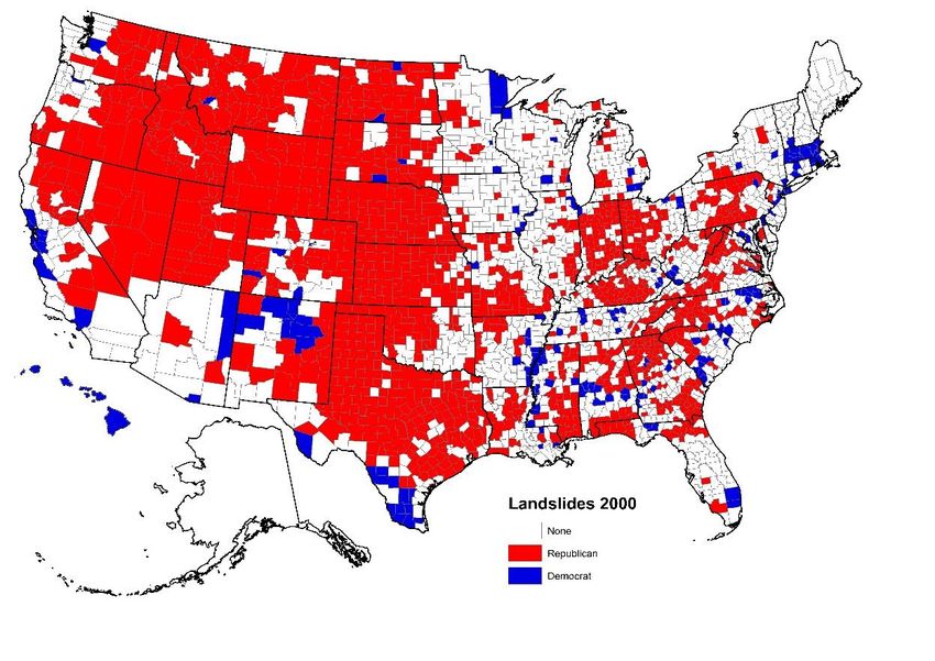
To evaluate and extend his claims, that same definition is deployed here: polarization is represented
by situations where one party’s candidate for the presidency defeats the other party’s candidate by
20 percentage points or more (of their combined, two-party vote total). If Bishop is correct, then the
number of places where this occurred should have increased over the sequence of seven elections
(1992-2016) for which we have data.4 Use of the 20 percentage points gap between the two
candidates is, of course, arbitrary but it is a useful threshold because very few counties won by that
margin by a party at one election were won by the opposing party at a later contest during this
period. Mapping the so-defined landslide counties thus provides a clear picture of those parts of the
country where one party dominates.

        Bishop’s basic empirical contention that at the county scale the United States has become
increasingly polarized in its voting for president is readily appreciated by a series of maps showing
those counties that were won by landslides over the sequence of seven elections beginning with Bill
Clinton’s 1992 victory over George H. W. Bush.5 A big change occurred between then and 2000,
when George W. Bush defeated Al Gore. Figure 1 shows that landslide victories characterised only a
minority of the counties in 1992: 19 per cent of them returned a Democratic landslide and another
19 per cent returned a Republican landslide, with neither party winning such a clear majority in the
remaining 62 per cent. The Republican landslides mainly occurred to the west of the Missouri,
covering much of Nebraska, western Kansas, Oklahoma and Texas plus major segments of Idaho,
Nevada and Utah (Balentine and Webster, 2018). Democratic Party landslides were more widely
spread, with clusters on the west coast and in the ‘Black Belt’ along the Mississippi in Arkansas,
Louisiana and Mississippi, as well as in Vermont, West Virginia and several areas with relatively large
Hispanic populations (along the Rio Grande border, for example).

        Eight years later, the map was very different (Figure 2). Many of the Democratic Party’s
landslides had disappeared; of the 525 counties Bill Clinton won by more than 20 percentage points
in 1992 only 172 returned a similar victory for Al Gore (he won by a landslide in only eight of the 45
counties where Bill Clinton did so in his home state of Arkansas): just sixteen switched to a
Republican landslide, however, and the remainder became more competitive. Only parts of southern
New England produced a substantial block of Democratic landslide counties. By contrast, much of
the map, especially west of the Missouri and extending across most of the Mountain states into
western California, Oregon and Washington, had turned red. There was also a very substantial
increase in the number of red counties to the east of the Mississippi, leaving only the counties of the
upper Midwest, New England and much of the eastern seaboard with relatively close results in that
election (a pattern also observed by Hopkins, 2017).

         That large block of red remained in place at the next three elections – 2004, 2008 and 2012
– and the only significant change was an increase in the number of Democratic landslides: Gore won
by that margin in just 192 counties in 2000, whereas Obama succeeded in doing so in 323 eight years
later, winning by the same margin again in 255 of them in 2012. Those successes were concentrated
along the eastern and western seaboards, in New England and in New Mexico: there was no return
to substantial Democratic hegemony in the Black Belt (Figure 3).

        The elections from 1992 to 2012 were part of what students of American politics call a
continuing sequence, of normal voting when most people retain their partisan preferences across

4
  We are grateful are grateful to Clark Archer, Fred Shelley and Bob Watrell for allowing us to use the county-
scale data set they compiled for presidential elections between 1992 and 2016 in this research (see Johnston
et al., 2016).
5
  These maps were created using a carefully-constructed data set by Clark Archer, Fred Shelley and Bob Watrel
for presidential elections between 1992 and 2016 in this research; we are grateful to them for sharing it with
us.

                                                       3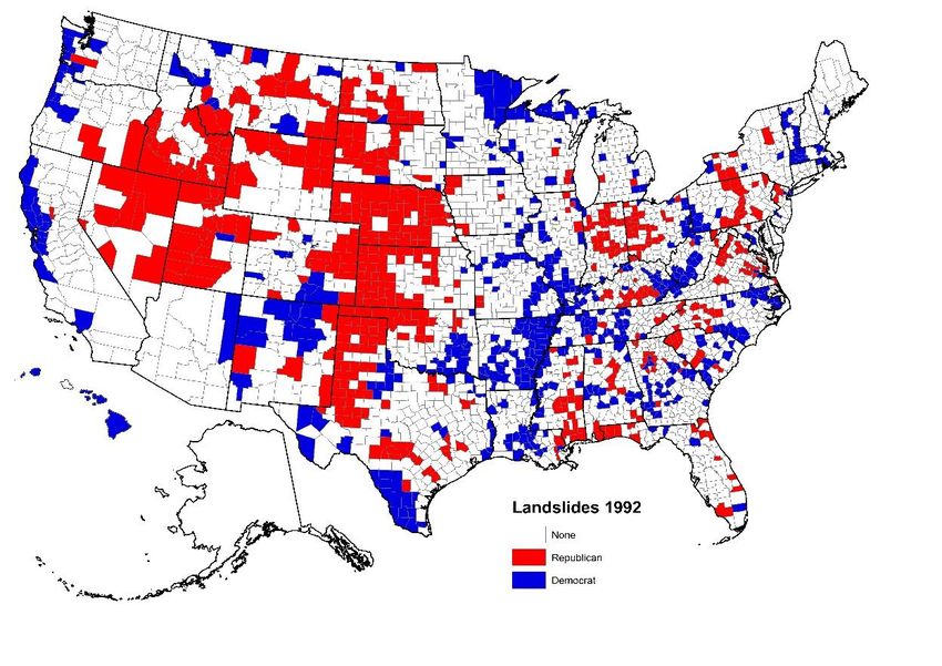
elections, producing a relatively constant electoral geography (Converse, 1976; Key, 1955; Archer
and Taylor, 1981). In this case, however, although the maps’ general pattern retained their same
shape (the areas of Republican and Democratic dominance were little changed) the topography
became more exaggerated with the larger number of landslide victories, especially for the
Republicans (Figure 4).
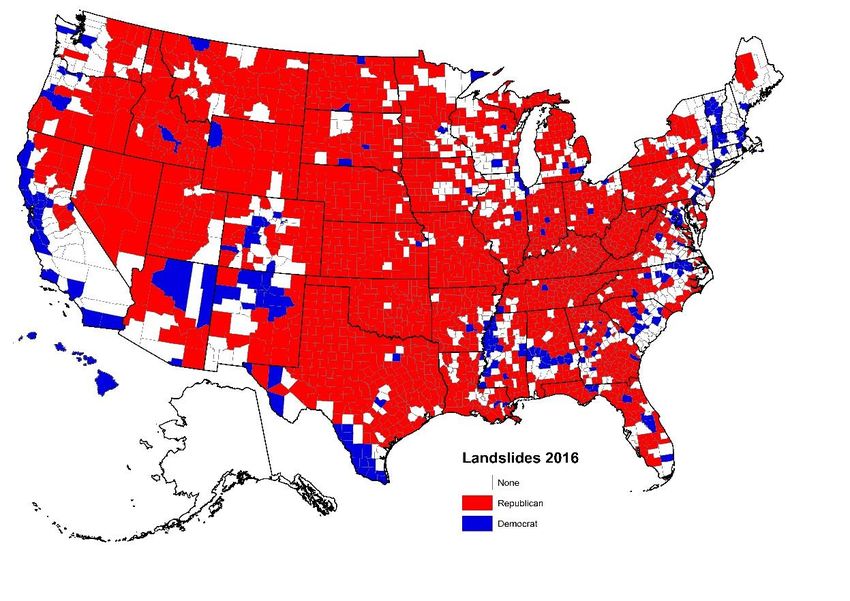
For some commentators, the 2016 election promised to be a deviation from that general
pattern, as Trump relatively successfully campaigned among the disadvantaged white working class
in areas where Republican landslides had previously been rare (much of the ‘Rustbelt’, for example).
He won by landslides again in almost every county where Romney had in 2012 (indeed, only eight of
those landslides were not repeated four years later), and added a further 507, mainly in the north-
east (other than New England). There was less change to the geography of Democratic landslides:
Hillary Clinton repeated Obama’s success in 202 of the 266 counties where he won by more than 20
points – and only one county that provided Obama with a landslide victory did so for Trump. (On the
2017 election as part of the continuing sequence see Johnston, Pattie et al., 2017.)
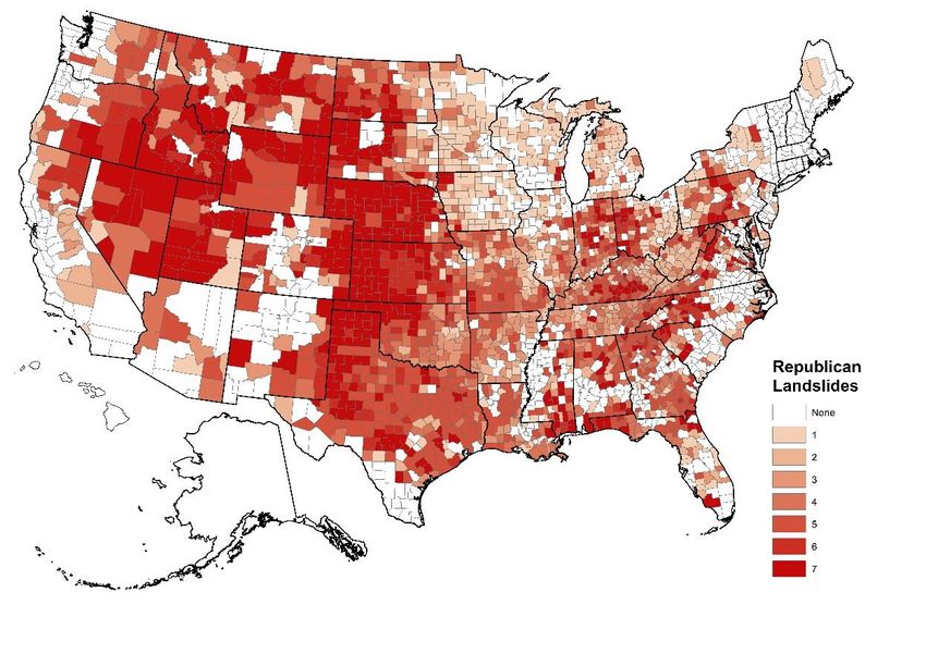
The very different geographies of landslide victories for the Republican and Democratic
Party candidates are clearly identified in the summary maps (Figures 5 and 6). For the Republicans, a
majority of counties west of the Missouri were won by landslides at six or seven of the elections
(Figure 5), as was also the case with many counties on the western fringe of the Appalachians and
parts of the ‘rust belt’ (notably in Indiana, Ohio and Pennsylvania). Once the Republicans gained a
landslide hold on a county they were very unlikely to lose it: of the 559 counties won by 20
percentage points or more in 1992, for example, only 28 were not won by that margin again in 2016
– and only two of those were Democratic landslide victories at the latter date. The Republicans won
by a landslide in 587 and 610 counties respectively in 1992 and 1996, and then in 1428 when George
W. Bush won his first election in 2000. Of the 725 counties won by a landslide then but not at the
previous two contests, 225 were won by a landslide by neither party in 2008 (Obama’s first victory)
but by 2016 only 36 did not return a landslide Republican victory. Having become the dominant
party in a county, the Republicans rarely saw their hegemony challenged in a contest where they
failed to win again by at least 20 percentage points.
The contrast between the two maps in Figures 5 and 6 is stark. That for the Democratic Party
has relatively few clusters of counties coloured dark blue, where its candidates won by more than 20
points at almost all of the seven elections. Apart from concentrations on the west coast, in New
Mexico, along the southern Mississippi, in central Alabama and much of New England (especially
Massachusetts and Vermont), there are also some areas (shown in the lighter blue) where the
Democrats won landslide victories at a few contests – in Maine, for example, and parts of Arkansas
(Bill Clinton’s home state); but much of the country is blank – large tracts of territory, even whole
states (Nebraska and Nevada), where the Democratic Party candidates failed to win a county by a
landslide at even one of the seven elections. The high point was in 1996, when there were 542
Democratic landslide wins. At the next election in 2000 this was reduced to just 192; there was a
recovery in 2008 and 2012, when Obama won landslides in 323 and 266 counties respectively, but
this fell back to 226 in 2016. Bill Clinton gained a landslide victory in 542 counties in 1996, but Hillary
Clinton won by a similar margin in only 165 of them in 2016, and she gained a landslide victory in
just 208 of the 323 where Barack Obama did in 2008.
This asymmetry in the number of landslide counties is further illustrated in Table 1, which
gives the percentage of the 3115 counties analysed here according to how many landslides they
recorded over the seven elections. Comparing the two parties, the difference is stark: whereas some
three-quarters of the counties returned a Democratic landslide at none of the contests, that was the
case for only just over one-quarter for Republican landslides. Similarly, whereas 20.4 per cent of
4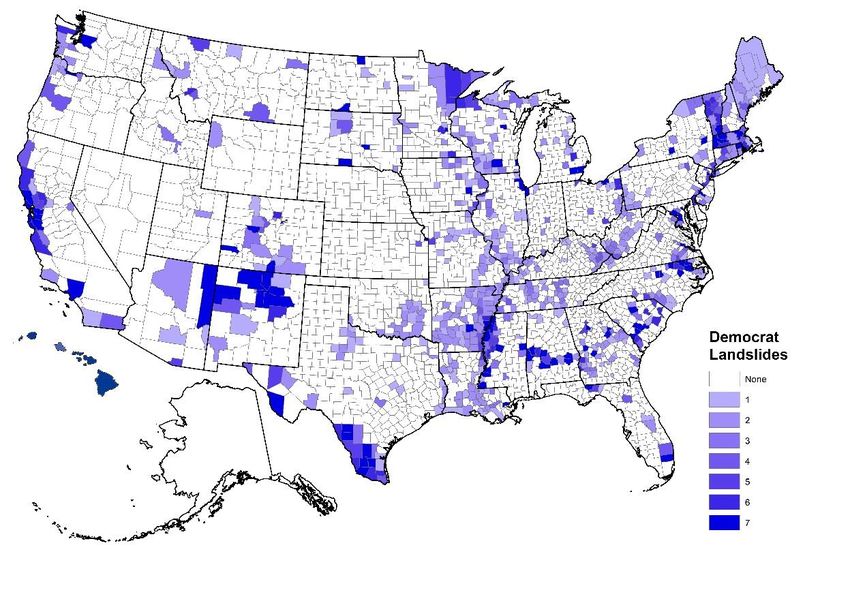
counties returned a Republican landslide on six or seven occasions, and 37.4 per cent on at least five,
the comparable figures for Democratic landslides were just 4.8 and 5.9 per cent.

         The maps indicate considerable geographical variation in the distribution of landslide
victories, therefore; this is encapsulated in Table 2 which shows the percentage of counties by the
number of landslides for each party and of no landslides, by the nine Census Divisions. Nearly one-in-
five of the counties returned a landslide for neither party at any election, for example, but that
varied from just over 8 per cent in the East North Central division to almost 47 per cent in the
Mountain division. Those returning no landslide at five or more of the seven elections formed more
than half of the total number of counties in the East North Central, Mid-Atlantic and New England
census divisions (i.e. the north-eastern parts of the country) and 45 per cent of the total in the
Pacific region. By comparison, 46.9 per cent of counties in the Mountain division returned a landslide
for one of the two parties at every election – in almost all cases for the Republican Party’s candidate.
Within that division, 52 per cent of counties in Idaho returned a landslide for one of the parties at
every election, as did 65 per cent of those in Utah and 77 per cent in Nebraska. These were
overwhelmingly delivered for the Republican candidate: only one county in Idaho regularly returned
a Democratic landslide; one Utah county did so at one election; and at none of the seven elections
did even a single Nevada county deliver a Democratic landslide. New England was the only division
at which over one-quarter of the counties returned a Democratic landslide at five or more of the
seven elections, and of the other divisions only in the Pacific did even 15 per cent of counties return
five or more Democratic landslides – a clear contrast to the five divisions where over 30 per cent of
counties returned a landslide at five or more elections for the Republicans.

A misleading cartography?

A sequence of Republican presidential candidates – George W. Bush, John McCain, Mitt Romney and
Donald Trump – painted an increasing proportion of the map of American counties red according to
this cartographic analysis. By 2016, 72 per cent of all counties returned a Republican landslide
victory, compared to just 7 per cent for the Democrats – leaving only just over one-fifth of the
country’s counties where the contest between the two parties was relatively close. But this
geography does not correspond with the overall outcome of that final election in the sequence,
when Hillary Clinton outvoted Donald Trump by 48.2 to 46.1 per cent. The reason, as several
commentators have pointed out, is misleading cartography; the Republicans tend to win by large
majorities in counties with relatively small populations – i.e. in rural and small-town America –
leaving the Democrats winning by similar margins in a much smaller number of counties with very
large populations – i.e. metropolitan America.

         This clear difference is illustrated by Table 3. The first block shows the mean number of
votes cast in each type of county at each election and illustrates a widening gap between the two
parties. In 1992, the average county won with a Democratic landslide had about three times as many
votes cast as the average county won with a Republican landslide; in 2016, the difference was
almost ten times. As the number of Republican landslide counties increased almost fourfold their
mean population increased by less than 20 per cent; Republican predominance was predominantly
in small town and rural America. For the Democrats, whereas the number of counties where Hillary
Clinton won by a landslide was less than half of the number won by Bill Clinton twenty-four years
earlier, the mean number of votes cast in those landslide counties grew by some 280 per cent over
the same period. Fewer places but more people – i.e. in the country’s large cities – delivered
Democratic landslides.

       This stark difference is brought into further relief in Table 3’s second block of data, which
shows the total number of votes cast in each type of county at each election. At the first two

                                                   5
contests, many more votes were cast in Democratic- than in Republican-landslide counties (over
three times as many in 1996). Although the gap closed thereafter, there were more voters in
Democratic- than Republican-landslide counties at each successive election except 2004; and despite
the massive difference in the number of counties won by landslides between the two parties’
candidates in 2016 they had almost the same number of votes. Red might outshine blue on the map,
but only because of the differences in the electorate of counties won by a landslide. Furthermore, as
the data in the first column of the second block in Table 3 show, more than half of the total number
of votes at every election until 2012 and 2016 were cast in counties that delivered a landslide to
neither candidate: purple America was numerically larger than either red or blue America, but was
increasingly unseen because those purple counties, too, had relatively large voting populations.
Reanalysing the map: a metropolitan-rural continuum
At the county scale, therefore, the polarization of America’s electoral geography appears to have
involved, in effect, a growing metropolitan-rural divide. To explore this further, counties have been
grouped according to a scheme developed by the National Center for Health Statistics (Ingram and
Franco, 2013). It has six categories:
Metropolitan
1. Large Central Metro – these counties are parts of Metropolitan Statistical Areas (MSAs) with
more than one million inhabitants: they either contain the entire population of the MSA’s
central cities; or have their entire population in the MSA’s largest central city; or contain at
least 250,000 of the population of one of the MSA’s principal cities.
2. Large Fringe Metro – these are counties in MSAs with more than one million inhabitants that
did not qualify as Large Central Metros (i.e. they are basically suburban areas of large
metropolises).
3. Medium Metro – all of the counties in MSAs with populations between 250,000 and
999,999.
4. Small Metro – counties in MSAs with less than 250,000 inhabitants.
Non-Metropolitan
5. Micropolitan – counties in defined micropolitan urban areas (with populations of 10,000-
49,999).
6. Noncore – all other counties (i.e. rural).
Table 4 shows the percentage of counties in each of those six categories that returned either a
landslide victory for one of the parties’ candidate or no landslide, at each election. The difference
between the two parties is again stark, and becomes starker over time. For the Democratic Party, as
one proceeds through the six categories, from the inner cities of major metropolitan areas through
their suburbs, the smaller cities and into small-town and rural America, the percentage of counties
returning a landslide declines, increasingly precipitately. Complementing that pattern, as one moves
down the columns so the percentage returning a Republican landslide increases. Democratic
landslides were especially characteristic of the central cities of large metropolitan areas – and
increasingly only so; Republican landslides increasingly dominated all other sections of America.
Further, and importantly, given that up to half of all Americans who cast votes lived there, whereas
at the early elections in the sequence there was little difference across the six categories in the
percentage of counties that delivered a landslide to neither party’s candidate, by 2016 their smaller
number was increasingly concentrated in the bigger places. The smaller places became more
polarized – almost entirely in favour of the Republican Party – whereas the largest places were
divided between Democratic landslides and counties where the two parties shared the votes
relatively equally.
6Those trends over time are clarified by comparisons along the rows in Table 5. For the Large
Central Metros, the later elections saw a not-inconsiderable increase in the percentage of counties
delivering a Democratic landslide (from 48.4 to 64.5) and a fall to zero in the corresponding
percentage of Republican landslides. The percentage of counties with no landslide also declined:
America’s central cities became increasingly-polarized, Democratic Party heartlands. In their suburbs
(the Large Fringe Metros), on the other hand, there was increasing polarization into Republican
landslides: the percentage of counties returning a Democratic landslide remained consistently small
– never more than 16 per cent – but the dominant pattern of relatively evenly-matched parties (in
1992, 63 per cent of these counties returned a landslide for neither party) was replaced by
Republican-dominated suburbia from 2000 on.
In the next two categories – the medium and small metropolitan areas – increased
Republican dominance was even more marked, as the percentage of counties with either
Democratic or, even more so, no landslide declined very substantially. This pattern was repeated in
the Micropolitan and NonCore (i.e. rural) areas where Republican landslides increased fourfold over
the period, Democratic landslides declined (precipitately in rural areas), and the percentage of
counties where neither party dominated over the other also fell very substantially. By 2016 83.7 per
cent of NonCore counties delivered a landslide victory for the Republican candidate, compared to
21.9 per cent twenty-four years earlier.
Changing the scale
The results discussed above conform to Bishop’s general argument regarding increased polarization
of the American electorate over recent decades – the trend he had observed continued over the
three further presidential elections in 2008, 2012 and 2016. The percentage of counties without a
landslide victory for either party’s candidate declined steeply from a little under 64 per cent in 1992
to just over 20 per cent in 2016. In that clear sense, the American electorate has become
geographically more polarized in its support for Republican and Democratic Party candidates.
That headline pattern has to be qualified somewhat, however. Although nearly four-in-five
counties returned a landslide victory for either Donald Trump or Hillary Clinton in 2016, nevertheless
more votes were cast in those counties where there was no landslide for either candidate than in
those where one or the other won by a margin of at least twenty percentage points. The modal US
county in 2016 saw a relatively close race between the two main parties’ candidates. Indeed, until
2012 more votes were cast in counties where there was no landslide victory than in a combination of
those where one of the two candidates had a landslide victory, and by 2016 just under 40 per cent of
all votes were still cast in the ‘no landslide’ counties.
Furthermore, the growth in landslide counties was asymmetric, in two ways. First, although
many more counties returned Republican than Democratic landslide majorities over the seven
elections, nevertheless at all but one of those contests (2004) more votes were cast in counties that
returned a landslide for the Democratic Party’s candidate than in those where the Republicans’
candidate prevailed by the same margin. Secondly, the growth in the number of Republican
landslides was very much concentrated in rural America, whereas in the metropolitan areas –
especially their central cities – there were very few such counties; those inner city, high density
areas were characterized, at all seven elections, by a combination of counties returning either a
Democratic landslide or no landslide. The dominant geographical element was thus, as others have
noted (Lichter and Ziliak, 2017), a growing metropolitan-urban-rural cleavage.
Those findings, though consistent with Bishop’s general arguments and analyses, are in an
important respect incommensurate with the more detailed features of his claims regarding the ‘big
7sort’. Much of his case regarding increased spatial polarization involves discussion of
neighbourhoods and similar geographical units that are typically very much smaller than the average
county: indeed, the average county in the central city of an MSA with a population of over one
million will contain a myriad separate – if often overlapping – neighbourhoods. For example, Bishop
(2009, 40) encourages his readers to
… look around: our own streets are filled with people who live alike, think alike, and vote
alike. This social transformation didn’t happen by accident. We have built a country where
everyone can choose the neighborhood (and church and news shows) most compatible with
his or her lifestyle and beliefs. And we are living with the consequences of this segregation
by way of life: pockets of like-minded citizens that have become so identically inbred that we
don’t know, can’t understand and can barely conceive of “those people” who live just a few
miles away.
His geographical terms – streets, neighborhoods, ‘pockets of like-minded citizens’ – refer to much
smaller areas than counties and although in some rural districts there may be relative uniformity
across substantial tracts of territory in their populations’ socio-economic and -demographic
characteristics, this is almost certainly not the case across a majority of metropolitan counties,
although many there may contain substantial blocks of contiguous neighbourhoods with similar
features. So what is the situation within counties?
To address this question, we use data for voting patterns by precincts. There is no central
aggregating agency for precinct-level election data in United States, nor is there in many states, so
collection of precinct-level results for the 2012 and 2016 presidential elections required contacting
the relevant electoral authorities in each state and county as needed. In most cases, state
Secretaries of State or Election Boards provided state-wide precinct results, but several states
required contacting each county’s electoral authority independently, namely Colorado, Indiana,
Michigan, Missouri, New Jersey, New York, and Pennsylvania. Kansas, Kentucky, Oregon, and West
Virginia required county-specific contact for a minority of counties. Most electoral authorities
provided results without charge via email or fax, but units such as Utah and many counties in
Missouri required fees for access to their data. The Harvard Election Data Archive supplied precinct-
level results for the 2008 presidential election. No data were available for earlier elections so in this
section we can only analyse the last three.
Because precinct boundaries are frequently changed – especially though not only when
there is a redistricting of electoral units, such as Congressional Districts – their number varied across
the three elections. There were 189,697 for the 2008 election, with a mean number of votes cast of
690. In 2012, there were 173,524 with a mean of 712 votes cast; and in 2016 the mean was 780,
across 173,526 precincts.
Table 6 shows the distribution of the three types of landslide at the precinct scale across the
six types of county, for the three elections. The first block shows the distribution across the rows –
i.e. each type within each year: thus, for example, 49.0 per cent of the precincts returning a
Democratic landslide in 2008 were in the Large Metro Central counties and 19.6 per cent were in the
Large Metro Fringe counties. The main feature of these figures is the absence of substantial change
across the three elections; the distribution of precincts returning a Democratic landslide across the
six types, for example, was little different in 2016 from the distribution in 2008.
The second block of data shows the percentage of precincts according to its landslide
category in each of the six types at each election – in 2008, for example, 59.4 per cent of all precincts
in Large Metro Central counties returned a Democratic landslide, for example, and 9.5 per cent
returned a Republican landslide. These percentages suggest greater change across the three
elections in most of the county types. The large metropolitan central cities – the first type – had just
8a small increase (of 4.5 percentage points) in the precincts returning Democratic landslides between
2008 and 2016 and an even smaller decline in the percentage returning landslides. Elsewhere, across
all five remaining types the dominant, and increasingly substantial, trend is for an increase in the
percentage of precincts returning a Republican landslide, especially between 2012 and 2016. That
percentage increased in the Micropolitan areas from 40.4 to 47.6 between the two Obama victories
of 2008 and 2016 and then jumped to 65.9 per cent in 2016; and in the Noncore (i.e. predominantly
rural) areas the increase was from 48.9 to 60.2 in the first inter-election period and then to 81.1 in
the second. The country’s inner cities swung slightly to the Democrats over the short period; in the
suburbs and beyond, there was a swing towards the Republicans while Obama remained in power
but when Trump faced Hillary Clinton that was magnified very considerably.
At the precinct scale, therefore – the scale of the neighbourhood on which most of Bishop’s
discussion, if not his data and maps, focused – the metropolitan-rural continuum again stands out.
The pattern changed very little in the metropolitan central cities over the three elections: a majority
of the precincts returned a Democratic landslide, less than one-tenth of all precincts returned a
Republican landslide, and there was a landslide for neither party in between one-quarter and one-
third of all precincts. In all of the other five types – from the suburbs of large metropolitan areas
through to the rural areas – the dominant change was a significant reduction in the percentage of
precincts that returned a landslide for neither party and a substantial increase in the percentage
delivering a landslide for the Republicans.
This lack of substantial change in the large metropolitan areas, especially their central cities,
between 2012 and 2016 is somewhat surprising, given that much of Trump’s campaign focused on
the relatively deprived, white working-class, many of whom lived in those places (Kivisto, 2017;
Ashcroft, 2017). To explore this further we used a statistical classification algorithm to group
together metropolitan areas (SMSAs) according to the percentage of their precincts at each of the
elections that returned no landslide, a Democratic landslide or a Republican landslide. Eight groups
were identified, and the average percentages for each are in Table 7. Of the 373 SMSAs for which we
have data, only 51 showed no appreciable change: eleven (group 1) had a Democratic landslide in
the great majority of their precincts at all three elections and forty similarly saw a Republican
landslide in most of their precincts at each contest. The third group of 92 SMSAs, which included
almost all of the country’s biggest cities, saw very little change in their profiles, with the largest
percentage of precincts delivering a Democratic landslide. The remaining five groups were all
characterised, to some extent, by an increase in the percentage of precincts that returned a
Republican landslide. By far the biggest absolute change in that direction was in the forty SMSAs in
the seventh group, where the percentage of Republican landslide precincts increased fourfold from
16 to 64. Many of those SMSAs are in the East North Central division – rustbelt places such as
Carbondale-Marion, IL, Evansville, IN-KY, Johnstown, PA, and Wheeling, WV-OH, where Trump
substantially extended the Republican’s dominance in many neighborhoods.
As the country’s smaller city, small town and rural counties became more predominantly
Republican in their voting for president, therefore, so an increasing share of their precincts returned
a landslide victory for the Republican candidates. In many metropolitan areas, on the other hand,
there was relatively little change in the percentage of precincts returning a landslide for one or the
other party’s candidate, but that was not the case where Trump made substantial inroads to the
Democratic Party’s dominance in some rustbelt – mainly smaller – metropolitan areas.
Within most large metropolitan areas change in the pattern of landslide victories was largely
concentrated in the suburban counties. This is illustrated by the fourteen-county Chicago-
Napierville-Elgin SMSA, thirteen of which are classed as Large Central Metro in the NCHS
classification and the remainder as Large Fringe Metro. They are split into three groups in Table 8:
9Cook County – the Large Central Metro which includes the City of Chicago; four counties which
border on Cook (the inner suburbs); and the nine ‘outer suburban’ counties. Very little changed in
Cook County over the three elections: over three-quarters of precincts returned a Democratic
landslide at each and there were virtually no Republican landslide precincts. The next group of four
counties – the ‘inner suburbs’ – are characterised, with the exception of Lake County (IN), by large
shares of precincts returning no landslide at any of the three elections and with only small
percentages returning Republican landslides. Finally, the main feature of the nine ‘outer suburban’
counties is the substantial increase in most in the percentage of precincts delivering a Republican
landslide – every precinct in two cases in 2016.
Discussion and conclusions
Bishop’s book The Big Sort introduced a linked pair of hypotheses to the study of the electoral
geography of the United States. Empirical investigations show that one of these – that the country is
becoming increasingly polarized, as shown by the patterns of voting for Democratic and Republican
Party candidates for the presidency – has considerable validity, both nationally and locally at a
variety of spatial scales. The second – that the polarization is linked to greater self-selection in
migration patterns: people are increasingly congregating together with those with whom they share
attitudes that are reflected in their voting behaviour – has, as yet, gained only muted support.
This paper has focused on the first of those hypotheses, using Bishop’s chosen measure of
polarization – the percentage of areas (counties in his case) won by a landslide majority of twenty
percentage points or more – to explore its geography in greater detail than presented in his book or
elsewhere (though see the atlases of recent elections: Brunn et al., 2010; Archer et al., 2014; Watrel
et al., 2018). Cartographically, it appears that over the period 1992-2016 the country not only
became increasingly polarized (more counties delivered a landslide victory for one of the party’s
candidates) but also that the main beneficiary of that trend was the Republican Party. Closer
examination showed that although it was indeed the case that more counties delivered a Republican
landslide, most of them were relatively small in their number of voters if not area and at all but one
of the seven elections studied more voters lived in counties that returned a Democratic rather than
a Republican landslide – and even more lived in counties that delivered a landslide for neither party.
Closer examination of the pattern of changes using a classification of counties showed that
the main change in the frequency of Republican landslides occurred outside the metropolitan areas,
especially their central cities. Whereas in most SMSAs the central cities were dominated by the
Democratic Party across all seven elections, with very few of them returning a Republican landslide,
an increasing number of suburban counties switched from delivering no landslide to one favouring
the Republicans and by 2016 a majority of counties beyond the metropolitan borders delivered such
a landslide. In the rural counties, fully 81 per cent of precincts gave the Republican candidate a
landslide victory then, although there were considerable geographical variations – for example, no
state in New England had more than 40 per cent of precincts in the fifth and sixth NCHS types
returning a Republican landslide, whereas in each of Idaho, Indiana, Kentucky, Missouri, Nebraska,
Nevada, North Dakota, Oklahoma, Pennsylvania, Tennessee, West Virginia and Wyoming that was
the case in over 90 per cent of precincts.
This rural-urban continuum in presidential voting patterns across most of the United States
has become more pronounced recently, with the Democratic Party increasingly attracting strong
support only in the major metropolitan areas, especially their central cities and some of their
suburbs: ‘where the suburbs start to resemble rural exurbia, and in the vast rural regions beyond,
Republicans find much friendlier territory’ (Scala and Johnson, 2017, 181). Residents in those
increasingly pro-Republican areas, including many who have retired there from the big cities, are
10more religious, less liberal in their attitudes (on same-sex marriage and abortion, for example) and
want stricter controls on immigration and immigrants – attitudes that make them more likely to
favour Republican candidates, especially Donald Trump (see Gorski, 2017). But most Americans live
in the country’s metropolitan areas and they, especially their suburbs given that there is already a
Democratic hegemony in most of the central cities, are likely to form the main battleground at
future elections. They are, however, the parts of the country, as this analysis has shown, which have
experienced least change recently. Bishop’s discussion of his polarization hypothesis focused on the
streets and neighbourhoods that are becoming more homogeneous and as a consequence more
likely to provide a landslide victory for one of the two parties. But in the country’s densely populated
cities the data presented here have found little evidence of more landslide victories at the precinct
(i.e. neighbourhood) scale over the last three elections. The big changes have been in some of the
less densely populated suburbs, in the smaller towns and cities, and in the rural areas, where the
number of Republican landslide victories has increased substantially but which – even in 2016 –
housed only 30 per cent of those who voted.
In his discussion of the growing ideological and attitudinal polarization of the American
electorate, Campbell (2016) asked whether the consequences of the divergence might include that
the country’s legislative bodies would become less representative, that governance of such a divided
country would become more difficult and less effective – and, if so, what could be done about it. His
discussion of those and other issues made no reference to the potential impact of the growing
spatial polarization outlined here – pitting metropolitan America (especially its large central cities
and their inner suburbs) against the rest of the country. One aspect of that spatial polarization which
could have an important influence on the ideological polarization of the country’s legislature is the
potential it offers for even more gerrymandering and the creation of safe seats, which in its turn
favours the selection and election of more ideologically extreme candidates. By indicating that it
knew of no judicial standard against which it could determine whether a districting map was a
gerrymander – unlike the situation with the numerical standard used to outlaw malapportionment –
a Supreme Court 2006 judgement encouraged more extensive gerrymandering. The Republican
Party capitalised on this in the redistricting exercises that followed the 2010 census (McGann et al.,
2016; see also Daley, 2016) and the Court’s 2018 judgements dismissing two further cases claiming
partisan – pro-Republican – gerrymandering will encourage its continued deployment, leading to a
more divided House of Representatives and make questions regarding both the institution’s
representativeness and the barriers to effective democratic government even more moot (Johnston,
2018).
Within the large literature on political polarization in the contemporary United States, the
issue of spatial polarization has received relatively little attention. Bishop’s book challenged that
situation, and the empirical evidence assembled over the last decade (notably at the state and
district scales by Hopkins, 2017), and extended here, has validated his general hypothesis. Spatial
polarization has increased – but the changing patterns are more nuanced, more geographically
variable, than a simple chasm opening up across the whole country. The changes outlined here
indeed indicate increased polarization but it has been more intense in some parts of the urban-rural
continuum, and in some parts of the country, than others.
References
Abrams, S. J. & Fiorina, M. P. (2012). “The Big Sort” that wasn’t: a sceptical re-examination. PS:
Political Science and Politics, 45 (2), 203-210.
11Ansolabehere, S., Rodden, J. & Snyder, J. M. Jr. (2006) Purple America. Journal of Economic
Perspectives, 20 (1), 97-118.
Archer, J. C. & Taylor, P. J. (1981) Section and party: political geography of American Presidential
Elections from Andrew Jackson to Ronald Reagan. Chichester: Research Studies Press.
Archer, J. C. et al. (eds.) (2014) Atlas of the 2012 Elections. Lanham, NJ: Rowman and Littlefield.
Ashcroft, M. A. (2017) Hopes and fears: Trump, Clinton, the voters and the future. London: Biteback
Books.
Balentine, M. D. & Webster, G. R. (2018). The changing electoral landscape of the western United
States. The Professional Geographer, 70 (4), 566-582.
Bishop, B. (2009). The Big Sort: Why the clustering of like-minded America is tearing us apart.
Boston: First Mariner Books.
Brunn, S. D. et al. (eds.) (2010) Atlas of the 2008 Elections. Lanham, NJ: Rowman and Littlefield.
Campbell, J. E. (2016) Polarized: making sense of a divided America. Princeton NJ: Princeton
University Press.
Cho, W. K. Tam, Gimpel, J. G. & Hui, I. S. (2013). Voter migration and the geographic sorting of the
American electorate. Annals of the Association of American Geographers, 103 (4), 856-870.
Cho, W. K. Tam, Gimpel, J. G. & Hui, I. S. (2018) Migration as an opportunity to register changing
partisan loyalty in the United States. Population, Space and Place, doi 10.1002/psp2218
Converse, P. E. (1976) The concept of a normal vote, in A Campbell, P. E. Converse, W. Miller and D.
Stokes (eds.), Elections and the political order. New York: Wiley, 9-39.
Daley, D. (2016). Ratf**ked: the true story behind the secret plan to steal America’s democracy. New
York: Liveright Books.
Florida, R. (2017) The new urban crisis: how our cities are increasing inequality, deepening
segregation, and failing the middle class – and What We Can Do About It. New York: Basic
Books.
Gimpel, J. G. & Hui, I. S. (2015). Seeking politically compatible neighbors? The role of neighbourhood
partisan composition in residential sorting. Political Geography, 48 (1), 130-142.
Gorski, P. (2017) Why evangelicals voted for Trump: a critical cultural sociology. American Journal of
Cultural Sociology, 5 (2), 338-354.
Hopkins, D. A. (2017) Red fighting blue: how geography and electoral rules polarize American
politics. Cambridge: Cambridge University Press.
Ingram, D. D. & Franco, S. J. (2013) 2013 NCHS urban-rural classification scheme for counties.
Hyattsville, MD: U.S. Department of Health and Human services, Centers for Disease Control
and Prevention, National Center for Health Statistics, DHHS Publication No.2014-1366.
12Johnston, R. J. (2018) America gerrymanders on – for the moment. The Political Quarterly, doi
10.1111/1467-923X.12592
Johnston, R. J., Jones, K. & Manley, D. (2018) An increasingly polarized America? In R. H. Watrel, R.
Weichelt, F. M. Davidson, J. Heppen, E. K. Fouberg, J. C. Archer, R. L. Morrill, F. M. Shelley &
K. C. Martis (eds.) Atlas of the 2016 Elections. Lanham, MD: Rowman & Littlefield, 104-110.
Johnston, R. J., Manley, D. & Jones, K. (2016). Spatial polarization of presidential voting in the United
States, 1992-2012: the “Big Sort” revisited. Annals of the American Association of
Geographers, 106 (5), 1047-1062.
Johnston, R. J., Pattie, C. J., Jones, K. & Manley, D. (2017). Was the 2016 United States’ Presidential
contest a deviating election? continuity and change in the electoral map – or “Plus ca
change, plus c’est la meme geographie”. Journal of Elections, Public Opinion and Parties, 27
(4), 369-388.
Key, V. O. Jr. (1955). A theory of critical elections. The Journal of Politics, 17 (1), 3-18.
Kinsella, C., McTague, C. & Raleigh, K. N. (2015). “Unmasking geographical polarization and
clustering: a micro-scalar analysis of partisan voting behaviour.” Applied Geography, 62 (3),
404-419.
Kivisto, P. (2017) The Trump PHENOMENON: HOW THE POLITICS OF POPULISM WON IN 2016.
Bingley: Emerald Publishing.
Lang, C. & Pearson-Merkowitz, S. (2015). PartisansSorting in the United States, 1972-2012: new
evidence from a dynamic analysis. Political Geography, 48 (1), 119-129.
Lichter, D. T. & Ziliak, J. P. (2017). The rural-urban interface: new patterns of spatial interdependence
and inequality in America. Annals of the American Association of Political and Social
Sciences, 672 (1), 6-25.
McDonald, I. (2011). Migration and sorting in the American ELECTORATE: EVIDENCE from the 2006
Cooperative Congressional Election Study. American Politics Research, 39 (4), 512-533
McGann, A. J., Smith, C. A., Latner, M. and Keena, A. 2016. Gerrymandering in America: the House of
Representatives, the Supreme Court, and the future of popular sovereignty. Cambridge:
Cambridge University Press.
Mummolo, J. & Nall, C. (2017). Why Partisans do not sort: the constraints on political segregation.
Journal of Politics, 79 (1), 45-59.
Murray, C. (2013) Coming apart. The state of white America, 1960-2010. New York: Crown Forum.
Myers, A. S. (2013). Secular geographical polarization in the American South: the case of Texas,
1996-2010. Electoral Studies, 32 (1), 48-62
Scala, D. J. & Johnson, K. M. (2017). Political polarization along the rural-urban continuum? The
geography of the presidential vote, 2000-2016. Annals of the American Association of
Political and Social Sciences, 672, 162-184.
13Watrel, R. H. et al. (eds.) (2018) Atlas of the 2016 Elections. Lanham, NJ: Rowman and Littlefield.
14Table 1. The percentage of counties according to the number of landslides recorded at the US
presidential elections, 1992-2016
0 1 2 3 4 5 6 7
No Landslides 18.2 8.2 20.3 12.1 9.9 8.8 12.2 10.1
Democratic Landslides 75.5 7.1 7.5 2.8 1.1 1.1 1.3 3.5
Republican Landslides 25.1 12.6 6.9 7.7 9.9 17.2 6.0 14.7
15Table 2. The percentage of counties according to the number of elections at which they delivered a
Democratic landslide, a Republican landslide or no landslide, by census division
Number of Elections
Division 0 1 2 3 4 5 6 7
Democratic Landslides
New England 16.4 17.9 22.4 6.0 10.4 4.5 9.0 13.4
Mid Atlantic 73.3 8.0 5.3 2.7 1.3 2.0 0.7 6.7
East North Central 77.3 9.8 5.9 3.0 0.0 1.1 0.9 1.8
West North Central 84.4 5.9 5.0 1.3 0.4 0.6 1.0 1.5
South Atlantic 75.3 5.6 6.7 4.7 0.9 1.3 1.4 4.2
East South Central 70.1 8.2 9.9 4.4 0.8 1.4 1.1 4.1
West South Central 69.4 9.4 14.3 2.1 0.9 0.9 1.1 2.1
Mountain 87.7 2.7 3.2 0.8 1.3 0.5 0.8 2.9
Pacific 69.3 4.4 3.6 2.9 4.4 2.2 2.9 10.2
TOTAL 75.5 7.1 7.5 2.8 1.1 1.1 1.3 3.5
Republican Landslides
New England 97.0 3.0 0.0 0.0 0.0 0.0 0.0 0.0
Mid Atlantic 45.3 20.0 6.0 2.7 9.3 6.7 5.3 4.7
East North Central 25.4 28.8 7.8 7.6 11.4 7.8 4.8 6.4
West North Central 13.7 23.6 8.0 7.8 8.4 14.3 8.6 15.6
South Atlantic 32.5 7.8 10.5 6.3 10.1 19.3 5.6 7.9
East South Central 18.7 6.6 9.1 11.9 16.8 19.2 4.7 13.2
West South Central 13.8 3.6 3.4 12.8 11.1 34.0 5.1 16.2
Mountain 18.0 4.3 2.7 2.9 5.9 14.7 7.5 44.0
Pacific 54.7 4.4 8.0 7.3 3.6 13.1 7.3 1.5
TOTAL 25.1 12.6 6.9 7.7 9.9 17.2 6.0 14.7
No Landslides
New England 13.4 9.0 4.5 10.4 6.0 25.4 14.9 16.4
Mid Atlantic 11.3 6.0 9.3 10.0 6.7 12.0 22.0 22.7
East North Central 8.2 5.7 9.4 11.9 14.0 13.5 24.7 12.6
West North Central 17.3 9.3 15.4 9.9 12.4 8.2 21.7 5.7
South Atlantic 12.1 7.4 22.0 12.5 11.9 10.6 8.5 15.0
East South Central 17.3 8.2 25.0 22.5 10.2 5.2 3.8 7.7
West South Central 18.5 10.2 41.3 12.3 7.0 4.5 3.6 2.6
Mountain 46.9 8.3 15.5 7.2 4.3 5.1 5.6 7.0
Pacific 11.7 10.2 15.3 8.0 10.2 11.7 8.8 24.1
TOTAL 18.2 8.2 20.3 12.1 9.9 8.8 12.2 10.1
16Table 3. The number of voters in ‘landslide counties’, 1992-2016
Type of landslide None Republican Democrat Total .
Mean number of votes cast
1992 26,093 14,473 44,604 27,036
1996 25,859 13,067 51,682 27,888
2000 38,253 15,329 121,524 32,809
2004 51,462 19,412 152,053 39,167
2008 49,185 15,776 123,136 41,852
2012 57,168 16,424 131,888 41,002
2016 79,938 17,281 169,872 41,487
Total number of votes cast
1992 51,220,295 8,510,223 23,462,140 83,192,568
1996 49,726,147 7,971,081 28,115,946 85,812,724
2000 55,733,983 21,889,521 23,332,700 100,956,204
2004 62,886,776 32,845,280 24,784,729 120,516,785
2008 66,596,774 22,038,784 40,142,371 128,777,929
2012 62,368,779 28,184,145 35,609,789 126,163,713
2016 50,441,178 38,312,901 38,900,702 127,654,781
17Table 4. The percentage of counties returning a Democratic or a Republican landslide, or no
landslide, at each presidential election 1992-2016, according to the NCHS classification of counties
No Dem Rep No Dem Rep
1992 1996
Large Central Metro 48.4 48.4 3.2 48.4 50.0 1.6
Large Fringe Metro 63.4 12.8 23.9 65.1 16.2 18.8
Medium Metro 71.0 13.4 15.6 65.3 18.0 16.7
Small Metro 71.1 14.6 14.3 69.7 13.1 17.1
Micropolitan 67.5 15.6 17.0 67.3 15.9 16.8
NonCore 58.9 19.2 21.9 57.4 18.5 24.1
TOTAL 63.8 17.1 19.1 62.5 17.6 19.9
2000 2004
Large Central Metro 46.8 45.2 8.1 50.0 41.9 8.1
Large Fringe Metro 49.4 8.0 42.6 41.2 5.4 53.4
Medium Metro 56.0 7.4 36.6 47.0 6.3 46.7
Small Metro 52.3 3.1 44.6 42.0 2.9 55.1
Micropolitan 49.5 5.2 45.3 41.4 4.4 54.2
NonCore 41.8 5.0 53.3 35.1 4.4 60.5
TOTAL 47.2 6.3 46.5 39.5 5.3 55.1
2008 2012
Large Central Metro 40.3 58.1 1.6 40.3 56.5 3.2
Large Fringe Metro 51.4 11.6 36.9 44.0 9.1 46.9
Medium Metro 49.7 13.9 36.3 45.1 11.7 43.2
Small Metro 47.4 9.4 43.1 37.4 7.1 55.4
Micropolitan 46.2 10.2 43.6 37.7 7.9 54.4
NonCore 38.5 7.4 54.0 28.6 6.2 65.2
TOTAL 44.0 10.5 45.5 35.5 8.7 55.9
2016
Large Central Metro 35.5 64.5 0.0
Large Fringe Metro 29.8 10.2 59.9
Medium Metro 33.6 9.0 57.4
Small Metro 26.3 6.3 67.4
Micropolitan 20.1 6.4 73.4
NonCore 12.2 4.1 83.7
TOTAL 20.5 7.4 72.2
18Table 5. Changes in the percentage of counties by landslide type and county type, 1992-2016.
1992 1996 2000 2004 2008 2012 2016
Large Central Metro
No Landslide 48.4 48.4 46.8 50.0 40.3 40.3 35.5
Democratic Landslide 48.4 50.0 45.2 41.9 58.1 56.5 64.5
Republican Landslide 3.2 1.6 8.1 8.1 1.6 3.2 0.0
Large Fringe Metro
No Landslide 63.4 65.1 49.4 41.2 51.4 44.0 29.8
Democratic Landslide 12.8 16.2 8.0 5.4 11.6 9.1 10.2
Republican Landslide 23.9 18.8 42.6 53.4 36.9 46.9 59.9
Medium Metro
No Landslide 71.0 65.3 56.0 47.0 49.7 45.1 33.6
Democratic Landslide 13.4 18.0 7.4 6.3 13.3 11.7 9.0
Republican Landslide 15.6 16.7 36.6 46.7 36.3 43.2 57.4
Small Metro
No Landslide 71.1 69.7 52.3 42.0 47.4 37.4 26.3
Democratic Landslide 14.6 13.1 3.1 2.9 9.4 7.1 6.3
Republican Landslide 14.3 17.1 44.6 55.1 43.1 55.4 67.4
Micropolitan
No Landslide 67.5 67.3 49.5 41.4 46.2 37.7 20.1
Democratic Landslide 15.6 15.9 5.2 4.4 10.2 7.9 6.4
Republican Landslide 17.0 16.8 45.3 54.2 43.6 54.4 73.4
NonCore
No Landslide 58.9 57.4 41.8 35.1 38.5 28.6 12.2
Democratic Landslide 19.2 18.5 5.0 4.4 7.4 6.2 4.1
Republican Landslide 21.9 24.1 53.3 60.5 54.0 65.2 83.7
19You can also read