Labor-Market Wedge under Engel Curve Utility: Cyclical Substitution between Necessities and Luxuries - Federal ...
←
→
Page content transcription
If your browser does not render page correctly, please read the page content below
Economic Quarterly— Volume 106, Number 1— First Quarter 2020— Pages 1–17

Labor-Market Wedge under
Engel Curve Utility: Cyclical
Substitution between
Necessities and Luxuries
Yongsung Chang, Andreas Hornstein, and Marios Karabarbounis

O
         ne of the leading research questions in macroeconomics con-
         cerns the identi…cation of the sources of economic ‡uctua-
         tions.1 Economists often identify these sources through ac-
counting procedures that are based on “wedges,” that is, violations of
a model economy’s equilibrium conditions conditional on data.2 For
example, representative agent models impose tight restrictions on the
comovement of consumption, hours, and real wages. For an optimal
allocation of consumption and hours worked, the marginal rate of sub-
stitution (MRS) between leisure and consumption has to equal the
real wage. Conditional on consumption, hours worked should increase
with the real wage, but for reasonable parameterizations of the rep-
resentative household’s preferences, this prediction is inconsistent with
observed movements in aggregate consumption, hours worked, and real
wages over the business cycle. On the one hand, the MRS increases
rapidly during expansions, as the marginal utility of consumption rel-

    We would like to thank Mark Bils, Pete Klenow, John Jones, Nicolas Morales,
    Mike Finnegan, and James Lee for helpful comments and suggestions. We thank
    Andrew Owens for his excellent research assistance. This work was supported by
    the National Research Foundation of Korea Grant funded by the Korean Govern-
    ment (NRF-2019S1A5A2A03043067). The views expressed in this article are those
    of the authors and not necessarily those of the Federal Reserve Bank of Rich-
    mond or the Federal Reserve System. E-mail: Yongsung.Chang@gmail.com; An-
    dreas.Hornstein@rich.frb.org; Marios.Karabarbounis@rich.frb.org.
    1
      See, for example, Christiano, Eichenbaum, and Evans (2005) or Smets and
Wouters (2007).
    2
      See Hall (1997) and Chari, Kehoe, and McGrattan (2007) for expositions of wedge
accounting.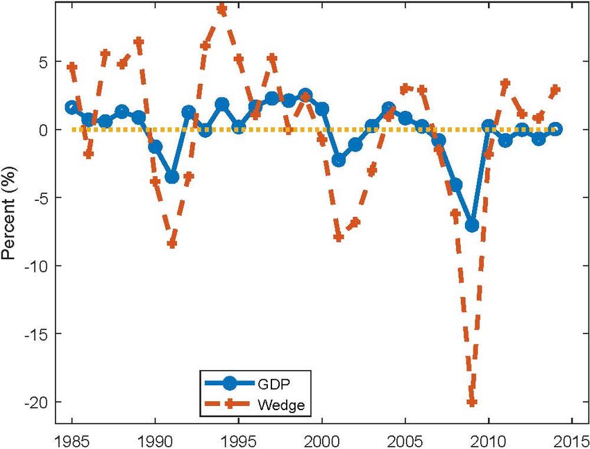
2                 Federal Reserve Bank of Richmond Economic Quarterly

ative to leisure quickly decreases, but on the other hand, there is no
corresponding strongly procyclical movement in real wages. This gap
between the MRS and the real wage, the so-called labor-market wedge,
when treated as an exogenous distortion is an important source of eco-
nomic ‡uctuations in this class of models.3 Of course, one would prefer
to explain the wedge rather than treat it as an exogenous shock.4
    Recently, Jaimovich, Rebelo, and Wong (2019) documented that
during the Great Recession, consumers reduced the quality of the goods
and services they consumed. Since part of the labor wedge is due to the
countercyclical marginal utility of consumption, procyclical variation of
quality can reduce the volatility of the labor wedge. While Jaimovich,
Rebelo, and Wong (2019) provide a general framework that includes
quantity-quality substitution, the measurement of quality is very chal-
lenging. Instead, in this paper we study the “average quality” e¤ects
stemming from composition changes in the household’s consumption
basket and nonhomothetic income-expenditure paths, that is, Engel
curves. It is straightforward to obtain information on the shape of En-
gel curves from cross-sectional data such as the Consumer Expenditure
Survey (CEX).
    We show that accounting for the substitution between necessities
and luxuries dampens the cyclical movement of the labor-market wedge
but only by a small amount. In booms, households’ consumption of
luxuries (e.g., food away from home) tends to increase relatively more
than the consumption of necessities (e.g., food at home). This sub-
stitution along the Engel curve slows down the increase in the MRS
because the marginal utility of consumption falls more slowly as con-
sumers move toward luxuries. For a parameterization of nonhomothetic
Engel curves consistent with the cross-sectional household expenditure
pattern across income quintiles in the CEX, we show that cyclical com-
position changes in the consumption basket can account for at most 16
percent of the volatility in the labor wedge measured in the aggregate
time series data.

     3
       Note that our (narrow) de…nition of the labor wedge represents only a part of the
broader de…nition of the labor wedge as the gap between the MRS and the marginal
product of labor. See, e.g., Bils, Klenow, and Malin (2018). Nevertheless, as Karabar-
bounis (2014) argues, our narrow wedge accounts for most of the volatility in the overall
wedge.
     4
       The existing literature o¤ers various interpretations for this wedge, including
changes in home-production technology, Benhabib, Rogerson, and Wright (1991), govern-
ment spending being a part of private consumption, Christiano and Eichenbaum (1992),
various frictions in the labor market, such as wage rigidity, Galí, Gertler, and Lopéz-
Salido (2007), or search frictions, Shimer (2010), and aggregation errors, Chang and Kim
(2007).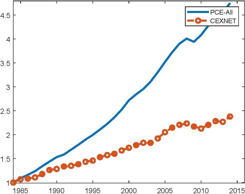
Chang et al.: Labor-Market Wedge under Engel Curve Utility                        3

    This article is organized as follows. Section 1 brie‡y discusses the
measurement of the labor-market wedge and lays out a simple model
where the household’s preferences exhibit an Engel curve. In Section
2, we compute the labor wedge corrected for the Engel curve, using
data on cross-sectional household expenditure patterns across income
quintiles in the CEX. Section 3 provides a concluding remark.

1.   LABOR-MARKET WEDGE
To understand the role of the Engel curve in the measurement of the
labor-market wedge, we …rst present the standard labor wedge for
household preferences expressed with respect to an aggregate consump-
tion good, C, and hours worked, H:
                              C 1 1=                 H 1+1=
                     U (C; H) =
                              1 1=                   1 + 1=
                        P C = W H;
where is the intertemporal elasticity of substitution (IES) for con-
sumption and is the Frisch elasticity of labor supply.5 The labor
wedge is de…ned as the ratio between the MRS (between leisure and
consumption) and the real wage (W=P ):
                       H 1=   M UL          W
                        1=
                            =      = M RS =   :                                 (1)
                      C       M UC          P
When we denote x ^ for the cyclical component of x (de-meaned growth
rate or percentage deviation from the trend), the cyclical component
of the labor wedge can be expressed as:
                            1 ^     1    \
                        ^= H     + C^ W=P:                        (2)

    Figure 1 shows the cyclical component of aggregate GDP and the
labor wedge for a baseline parameterization of preferences using ag-
gregate time series data. The measured wedge is highly volatile and
procyclical because: (i) hours worked and consumption are both pro-
cyclical, with hours being very volatile, and (ii) the real wage is neither
highly procyclical nor volatile. As shown in the table of Figure 1, (i)
hours are slightly more volatile than GDP and highly procyclical with a
0.95 elasticity with respect to GDP growth, while (ii) consumption and
the real wage exhibit similar volatility, and the real wage is only mildly
procyclical with a mere 0.19 elasticity with respect to GDP growth.

    5
      Since the labor-market wedge is entirely based on the intratemporal optimality
condition, we abstract from the dynamic decisions of households, e.g., savings, etc.
4 Federal Reserve Bank of Richmond Economic Quarterly
As a result, the labor wedge is tightly correlated with GDP and more
than twice as volatile: a 1 percent increase in GDP is associated with
a nearly 2 percent increase in the labor wedge for our baseline parame-
terization, = 0:5 and = 1.
We believe our baseline parameterization is plausible since (i) there
is ample evidence for an IES in consumption that is much smaller than
one, and (ii) variations in aggregate hours re‡ect the extensive margin
as well as the intensive margin of labor-supply decisions.6 In addition,
we obtain similar results for the labor-wedge volatility for a range of
empirically plausible values of and , see columns (2) through (5) in
Table 2.
Now, suppose that the household purchases N types of consumption
goods, fc1 ; :::; cN g, at prices fp1 ; :::; pN g. The household maximizes a
utility function with intertemporal elasticities of substitution that di¤er
across goods
N
X 1 1=
ci i
H 1+1=
U (c1 ; ::; cN ; H) = i
1 1= i 1 + 1=
i=1
XN
P m Cm = pi ci = W H;
i=1
where P m and C m represent the measured aggregate price and con-
sumption index. The FOCs are
1= i
i ci = pi ; for i = 1; :::; N (3)
1=
H = W;
where is the marginal utility of nominal expenditures. This speci…-
cation yields nonhomothetic Engel curves across goods. A good with
a small i is a necessity (e.g., food) whose marginal utility decreases
rapidly with increased consumption. A good with a large i is a lux-
ury whose marginal utility decreases slowly. Consequently, as total
expenditures increase for …xed prices and the marginal utility of ex-
penditures decline, consumption of luxury goods increases faster than
does consumption of necessities.
Summing over the FOCs for the consumption goods, we get the
marginal utility of expenditures
P 1 1= i X
iPi ci c~ 1 1= i
= = m m
with c
~ i ci : (4)
p c
i i i P C
i
6
For example, Havránek (2015) in a meta analysis of 169 published articles …nds a
mean estimate of 0.5 for the IES, and Keane and Rogerson (2012) discuss the relevance
of intensive and extensive margins for estimates of the aggregate labor-supply elasticity.Chang et al.: Labor-Market Wedge under Engel Curve Utility 5
Allowing for a labor wedge in equation (3) and using the marginal
utility of expenditures, the true labor wedge, , is then de…ned by the
expression
Cm M UL C m W
H 1== = : (5)
c~ c~ Pm
Compared to the standard measure of the labor wedge in (1) with
aggregate consumption, this wedge with multiple goods is likely to
be less cyclical because in economic booms households’ consumption
moves toward luxuries whose marginal utility decreases more slowly.
The cyclical component (growth rate) of the labor wedge is7
1 ^ X 1
^ = H + C^ m 1 ! i c^i W=P\m ; (6)
i i
P P
where C^ m = i ! i c^i and P^ m = i ! i p^i are Divisia quantity and price
indices of aggregate consumption. Measured quantity and price indices
of aggregate consumption are essentially constructed as Divisia indices.
Using these quantity and price measures of aggregate consumption in
expression (2), we obtain the di¤erence between the measured wedge
and true wedge
X N
X X
1 1 1 1
^m ^ = 1 ! i c^i 1 ! i c^i = ! i c^i :
i i i=1 i i
2. EMPIRICAL ANALYSIS
Engel Curves from the CEX
We use eight categories of household expenditures in the CEX: food
at home, food away from home, transportation (excluding vehicle pur-
chases), housing, health care, apparel, entertainment, and cash contri-
bution. In Table 1, …rst and second column, we report their expenditure
shares in 2005 and 2015. The expenditure shares of the eight categories
are quite stable over the decade, and in total (CEX8) they make up
about 75 percent of total expenditures— which is close to 89 percent of
the consumption-related expenditure (total expenditure net of those on
personal insurance and pensions, CEXNET). We exclude vehicle pur-
chases because vehicles are durable goods, and we exclude “insurance
and pensions”because they may re‡ect the household’s savings rather
than consumption.
7
^ P 1
From the de…nition of c~ in equation (4), we get c~ = i 1 ! i c^i ; where ! i
i
is the expenditure share of the ith good.6 Federal Reserve Bank of Richmond Economic Quarterly
For each consumption category i, the Engel curve parameter, i ,
can be estimated as follows. The FOCs of the household’s utility max-
imization for consumption goods (3) imply that for any two goods,
i
ln ci = ln cj i ln(pi =pj ): (7)
j
Let cQk
i denote the quantity of consumption for category i by the house-
hold in the kth quintile of the income distribution. Assuming that
households face the same prices, we get
! Q5
!
pi cQ5
i i p j cj
ln = ln ; (8)
pi cQ1
i j pj cQ1
j
and we can infer the relative Engel curves between categories i and j,
i = j , from the cross-sectional nominal consumption ratios of the re-
spective categories for households in the …fth and …rst income quintiles.
Based on the cross-sectional CEX of 2005 and 2015, we compute
the relative (to total expenditure) Engel curve parameters, si , third
and fourth column of Table 1,
ln pi cQ5 Q1
i =pi ci
si = : (9)
ln (P C Q5 =P C Q1 )
The relative Engel curve parameters for the two years di¤er somewhat,
but they do not change much over the decade, and their ranking stays
roughly constant. The last column of Table 1 displays the average
relative Engel curve parameters for the two years, which we use in our
calculation of the composition-adjusted labor wedges.
For a given aggregate intertemporal elasticity of substitution, we
calculate the levels of the corresponding Engel curve parameters as i =
si . The measured relative Engel curve parameters indicate an above
(below) average response of a category’s consumption to an increase of
income for si > 1(< 1). The average relative parameter is about 1:1,
thus the average Engel curve parameter is close to .
While the CEX contains information that we can use to calculate
the slope of household Engel curves, it does not contain information
on prices, and it is well-known that aggregate nominal expenditures
from the CEX and the more widely used NIPA Personal Consumption
Expenditures (PCE) diverge over time. For the prices of CEX con-
sumption categories, we use the corresponding price index from the
CPI, except for “entertainment” and “cash contribution.” For the lat-
ter two categories, we use the aggregate CPI since the CPI does not
have separate price indexes for them. Aggregate nominal CEX expen-
ditures are growing at a much slower pace than aggregate PCE in the
NIPA because the CEX systematically understates durable goods andChang et al.: Labor-Market Wedge under Engel Curve Utility 7
luxuries in households’ expenditures. Figure 2 shows that aggregate
PCE increased 4.6 times from 1985 to 2015, whereas aggregate CEX
expenditures (CEXNET) has increased 2.4 times. We, however, focus
on the cyclical components of consumption, and the de-meaned growth
rates of the two consumption aggregates comove fairly closely, as shown
in Figure 3. The correlation coe¢ cient for the two consumption growth
rates is 0.45, and the projection of the growth rates of aggregate PCE
on those of aggregate CEX yields an R2 of 0.80.
Cyclical Behavior of Labor-Market Wedges
We …rst show that the cyclicality of the labor-market wedge constructed
with our aggregate measure of consumption from the CEX is compa-
rable with that of labor wedges constructed from more standard mea-
sures of aggregate consumption. We then show that the labor wedge
constructed from the disaggregated CEX categories is less cyclical than
the labor wedge from the CEX aggregate. We start with our baseline
parameterization and then show that similar results obtain for other
empirically reasonable parameterizations.
The …rst column of Table 2 displays the cyclicality of the labor
wedge for our baseline parameterization and di¤erent measures of con-
sumption.8 The …rst three rows of Table 2 display the cyclicality of
the labor wedge based on the standard single-goods utility for three
measures of aggregate consumption: all items of PCE in the NIPA,
“PCE-All,” nondurable goods and services PCE, “PCE-NDS,” and a
Divisia-Aggregate of our eight CEX expenditure categories, “CEX8-
Aggregate.”The PCE-All is more cyclical than the PCE-NDS, but since
our framework applies to nondurable goods, the PCE-NDS is the ap-
propriate aggregate consumption measure. The labor wedge cyclicality
from the CEX8-Aggregate and the PCE-NDS are of similar magnitude,
with the CEX8-Aggregate-based labor wedge slightly less cyclical.
We now use the eight CEX consumption categories and construct
a labor wedge, “CEX8-Engel,” that allows for di¤erences in income
expansion paths of consumption (fourth row of Table 2). Comparing
CEX8-Engel with CEX8-Aggregate, we can see that accounting for dif-
ferences in income elasticities across commodities reduces the volatility
of the labor wedge by 9.3 percent. In other words, recognizing the di¤er-
ences in marginal utility across commodities together with the procycli-
cal/countercyclical nature of luxuries/necessities makes true marginal
8
Again, as in Figure 1, “cyclicality” is de…ned as the regression coe¢ cient of the
labor-market wedge growth rate on the GDP growth rate.8 Federal Reserve Bank of Richmond Economic Quarterly
utility move less than is implied by the usual aggregate consumption
measure and results in a less volatile labor wedge.
In the remaining columns of Table 2, we report the cyclicality of the
labor wedge based on alternative values of the preference parameters
and . Using a smaller intertemporal elasticity of consumption magni-
…es the labor-wedge cyclicality— it is even harder to justify the cyclical
behavior of consumption and hours as an optimal choice of the stand-in
household. With = 0:1, the cyclicality based on the CEX8-Aggregate
increases to 4.55— the wedge moves …ve times as much as GDP over
the business cycle. The cyclicality of the “true”wedge (CEX8-Engel) is
3.85, roughly 16 percent smaller than the standard measure. Using the
larger value, = 1, that is, log utility in consumption, accounting for
nonhomothetic Engel curves reduces the wedge cyclicality by only 6.2
percent. A larger labor-supply elasticity reduces the cyclicality of the
wedge because the marginal utility of leisure increases at a slower rate
in booms. The same reduction in the cyclicality of the marginal util-
ity of consumption from using disaggregated Engel curves then implies
a larger percentage reduction in the labor-wedge cyclicality. Overall,
correcting the movement of the marginal utility of consumption based
on the di¤erences in the Engel curve across the eight consumption cat-
egories in the CEX decreases the cyclicality of the wedge by 6 percent
to 16 percent; see row (6) of Table 2.
We obtain an upper bound on how much one can reduce the labor
wedge through modi…cations of the marginal utility of consumption by
making the marginal utility of consumption a constant, = 1; equa-
tion (2) and row (5) of Table 2. From equation (2) it follows that this
speci…cation provides an upper bound for any speci…cation of prefer-
ences for which the implied consumption index and labor supply are
positively correlated and the real wage is essentially acyclical.9 For ex-
ample, with = 1 and = 0:5, assuming a constant marginal utility of
consumption reduces the estimated cyclicality of the wedge by half rel-
ative to the benchmark case. Our treatment based on nonhomothetic
Engel curves across eight categories in the CEX materialize 18.5 per-
cent of this potential reduction in the cyclicality of wedge. Note also
that the relative contribution of our correction of the wedge remains
at 18.5 percent regardless of ’s and ’s; see row (8) of Table 2. In
the Appendix we show that this feature is a consequence of …xing the
relative Engel curve parameters and de…ning their levels proportional
to the aggregate intertemporal elasticity of substitution.
9
In particular, it includes preference speci…cations with a quality-quantity trade-o¤
along the lines of Jaimovich et al. (2019).Chang et al.: Labor-Market Wedge under Engel Curve Utility 9
3. CONCLUDING REMARK
Estimated DSGE models have been widely used to study economic
‡uctuations. One popular way to identify the sources of ‡uctuation in
these DSGE models is to measure shocks as “wedges”in model-implied
relationships among key aggregate time series, e.g., an optimality con-
dition or a resource constraint. According to this method, the labor-
market wedge— the gap between the real wage and the MRS between
consumption and leisure— often emerges as an important source of ag-
gregate ‡uctuations.
In this article, we have studied the extent to which procyclical
changes in the “average quality”of aggregate consumption can account
for the volatility of the labor wedge when Engel curves are nonhomo-
thetic. Using information on changes in consumption patterns from
the CEX, we have found that the impact of these composition e¤ects
on the labor wedge is of limited quantitative importance. They can
account for at most 6 percent to 16 percent of the labor-wedge volatil-
ity. We have also derived an upper bound on how much more general
approaches that allow for unobserved quantity-quality substitution in
consumption, such as Jaimovich et al. (2019), can reduce volatility of
the measured labor wedge. These more general speci…cations of pref-
erences can reduce the cyclicality of the labor wedge by at most 80
percent. The particular preferences we consider, nonhomothetic Engel
curves disciplined by the cross-sectional Engel curves over eight expen-
diture categories in the CEX, can account for only one-…fth of that
maximal reduction.10 Federal Reserve Bank of Richmond Economic Quarterly
REFERENCES
Benhabib, Jess, Richard Rogerson, and Randall Wright. 1991.
“Homework in Macroeconomics: Household Production and
Aggregate Fluctuations.” Journal of Political Economy 99
(December): 1166–87.
Bils, Mark, Peter J. Klenow, and Benjamin A. Malin. 2018.
“Resurrecting the Role of the Product Market Wedge in
Recessions.” American Economic Review 108 (April): 1118–46.
Chang, Yongsung, and Sun-Bin Kim. 2007. “Heterogeneity and
Aggregation: Implications for Labor-Market Fluctuations.”
American Economic Review 97 (December): 1939–56.
Chari, V.V., Patrick J. Kehoe, and Ellen R. McGrattan. 2007.
“Business Cycle Accounting.” Econometrica 75 (May): 781–836.
Christiano, Lawrence J., and Martin Eichenbaum. 1992. “Current
Real-Business-Cycle Theories and Aggregate Labor-Market
Fluctuations.” American Economic Review 82 (June): 430–50.
Christiano, Lawrence J., Martin Eichenbaum, and Charles Evans.
2005. “Nominal Rigidities and the Dynamic E¤ect of a Shock to
Monetary Policy.” Journal of Political Economy 113 (February):
1–45.
Galí, Jordi, Mark Gertler, and J. David Lopéz-Salido. 2007.
“Markups, Gaps, and the Welfare Costs of Business Fluctuations.”
Review of Economics and Statistics 89 (February): 44–59.
Hall, Robert E. 1997. “Macroeconomic Fluctuations and the
Allocation of Time.” Journal of Labor Economics 15 (January)
Part 2: s223–s250.
Havránek, Tomá¼ s. 2015. “Measuring Intertemporal Substitution: The
Importance of Method Choices and Selective Reporting.” Journal
of the European Economic Association 13 (December), 1180–204
Jaimovich, Nir, Sergio Rebelo, and Arlene Wong. 2019. “Trading
Down and the Business Cycle.” Journal of Monetary Economics
102 (April): 96–121.
Karabarbounis, Loukas. 2014. “The Labor Wedge: MRS vs. MPN.”
Review of Economic Dynamics 17 (April): 206–23.Chang et al.: Labor-Market Wedge under Engel Curve Utility 11 Keane, Michael, and Richard Rogerson. 2012. “Micro and Macro Labor Supply Elasticities: A Reassessment of Conventional Wisdom.” Journal of Economic Literature 50 (June), 464–76. Shimer, Robert. 2010. Labor Markets and Business Cycles. Princeton, N.J.: Princeton University Press. Smets, Frank, and Rafael Wouters. 2007. “Shocks and Frictions in U.S. Business Cycles: A Bayesian DSGE Approach.” American Economic Review 97 (June): 586–606.
12               Federal Reserve Bank of Richmond Economic Quarterly

APPENDIX

We can rewrite the equations for the growth rates in the measured,
true, and limiting labor wedge with = 1, as follows
                                                  1 ^m
                           ^m = ^1 +               C ;
                                                  1^
                           ^     = ^1 +            C ;
                                       1^          \m ;
                           ^1 =         H          W=P
             P
where C^ = si 1 ! i c^i .
    In Table 2, we list the regression coe¢ cients of the growth rate in
the three labor wedges on GDP growth in rows (3), (4), and (5). Across
columns the aggregate IES and labor supply elasticity change, but the
relative IES across categories, si , remain …xed. This means that the
                               \m , C^ m , and C^ , are all independent
                            ^ W=P
right-hand side variables, H,
of and .
    The regressions asymptotically re‡ect the linear projections of the
labor wedges on output
                                             1                                   1
     (3) :   E [^m j^
                    y] =   E[^1 j^
                                 y] +            E[C^ m j^
                                                         y] =        1
                                                                            +        m
                                                                                          y^;

                                             1                                   1
     (4) :   E [^ j^
                   y] =     E[^1 j^
                                  y] +           E[C^ j^
                                                       y] =          1
                                                                            +            y^;

     (5) :   E [^1 j^
                    y] =                                            1
                                                                            y^
Therefore the ratios in rows (6), (7), and (8) are given by
                                                                     m
                               (4)                         (             )=
             (6) :                    1=                        1       m
                               (3)                                 +     =
                               (5)                               (1= ) m
             (7) :                    1=                        1
                               (3)                                + m=
                                                                         m
                                     (6)
             (8) :                       =                          m
                                     (7)
As you can see, the relative improvements are independent of :
Chang et al.: Labor-Market Wedge under Engel Curve Utility 13
Figure 1 Cyclical Behavior of the Labor-Market Wedge
GDP H C W/P Wedge ( )
SD (%) 2.06 2.34 1.31 1.50 4.55
Cyclicality 1.00 0.95 0.56 0.19 1.88
Notes: Aggregate consumption (C) and its price are based on personal consump-
tion expenditure (PCE) data for nondurables and services from the NIPA. Ag-
gregate hours (H) and nominal wages (W ) are total hours and wages from the
BLS’s Labor Productivity and Cost index (LPC) for nonfarm business sectors
(https://www.bls.gov/lpc/). We use annual data and calculate their growth rates
as 100 times …rst di¤erences in logs. The labor-market wedge is computed for
=0:5 and =1. SD denotes the standard deviation, and “Cyclicality” denotes
the regression coe¢ cient on GDP growth.14 Federal Reserve Bank of Richmond Economic Quarterly Figure 2 Nominal Consumption Expenditures Note: Nominal expenditures of personal consumption expenditure of all categories (PCE-All) and those of CEX net of pension and insurance (CEXNET).
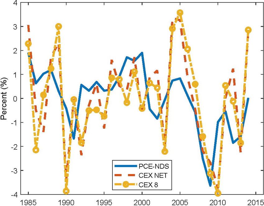
Chang et al.: Labor-Market Wedge under Engel Curve Utility           15

Figure 3 Cyclical Components of Consumption

Note: Real consumption growth of PCE nondurables and services (PCE-NDS),
CEXNET, and CEX8.
16              Federal Reserve Bank of Richmond Economic Quarterly

Table 1 Relative Engel Curves

[-1.5ex] Category                    Share (%)          Relative Engel (   i
                                                                               )
                                    2005      2015     2005     2015           Avg.
Food at Home                         7.1       7.2     0.78      0.68          0.73
Food away from Home                  5.7       5.4     1.30      1.15          1.23
Transportation                      10.3       9.9     1.28      1.18          1.24
Housing                             32.6      32.9     1.10      1.01          1.06
Health Care                          5.7       7.8     0.84      0.95          0.90
Apparel                              4.1       3.3     1.23      1.12          1.18
Entertainment                        5.1       5.1     1.45      1.13          1.29
Cash Contribution                    3.5       3.2     1.64      1.29          1.47
Sum of 8 Categories (CEX8)         73.8      75.1         –         –             –
Others                              15.0      13.6        –         –             –
Sum of All Above (CEXNET)          88.8      88.7         –         –             –
Personal Insurance and Pension      11.2      11.3     2.82       2.5          2.66
All Items                          100.0     100.0     1.00      1.00          1.00

Notes: The data are based on the annual overall expenditure shares and mean
expenditures of the …rst and …fth income quintiles (before taxes) from the Con-
sumer Expenditure Surveys of 2005 and 2015. “Transportation” excludes vehicle
purchases. “Others” are other miscellaneous categories and “Cash Contribution”
is cash donation.
Chang et al.: Labor-Market Wedge under Engel Curve Utility 17
Table 2 Cyclicality of Labor Wedges
[-1.5ex] Consumption Measure = 0:5 = 0:1 =1 = 0:5 = 0:5
for Marginal Utility =1 =1 =1 =2 = 0:5
(1) PCE-All 2.15 7.71 1.46 1.68 3.10
(2) PCE-NDS 1.88 6.35 1.32 1.40 2.83
(3) CEX8-Aggregate 1.52 4.55 1.14 1.05 2.47
(4) CEX8-Engel 1.38 3.85 1.07 0.90 2.33
(5) Constant M UC 0.76 0.76 0.76 0.29 1.71
(4)
(6) (3)
1 -9.2% -15.4% -6.2% -13.4% -5.7%
(5)
(7) (3)
1 -50% -83% -33% -73% -31%
(6)
(8) (7)
18.5% 18.5% 18.5% 18.5% 18.5%
Notes: Rows (1) through (5) display the regression coe¢ cient of labor-market
wedge growth rates on GDP growth rates for di¤erent measures of consumption in
the construction of marginal utility of consumption (M UC ). Rows (1) and (2) use
personal consumption expenditures (PCE) from the NIPA, all categories or non-
durable goods and services only. Rows (3) and (4) use the eight categories in the
CEX, where CEX8-Aggregate uses the Divisia-Aggregate and CEX8-Engel uses
the CEX8-Components together with the relative Engel curve parameters from
the last column of Table 1. Row (5) considers the limit for large, when M UC
is a constant and independent of the measure of consumption.You can also read