Learning Without a Global Clock: Asynchronous Learning in a Physics-Driven Learning Network
←
→
Page content transcription
If your browser does not render page correctly, please read the page content below
Learning Without a Global Clock:
                                                                         Asynchronous Learning in a Physics-Driven Learning Network
                                                                                 J. F. Wycoff, S. Dillavou, M. Stern, A. J. Liu, and D. J. Durian
                                                                       Department of Physics and Astronomy, University of Pennsylvania, Philadelphia, PA 19104
                                                                                                       (*dillavou@upenn.edu)
                                                                                                      (Dated: January 14, 2022)
                                                                  In a neuron network, synapses update individually using local information, allowing for entirely decentralized
                                                               learning. In contrast, elements in an artificial neural network (ANN) are typically updated simultaneously using
                                                               a central processor. Here we investigate the feasibility and effect of asynchronous learning in a recently intro-
                                                               duced decentralized, physics-driven learning network. We show that desynchronizing the learning process does
                                                               not degrade performance for a variety of tasks in an idealized simulation. In experiment, desynchronization ac-
arXiv:2201.04626v1 [cond-mat.soft] 10 Jan 2022

                                                               tually improves performance by allowing the system to better explore the discretized state space of solutions. We
                                                               draw an analogy between asynchronicity and mini-batching in stochastic gradient descent, and show that they
                                                               have similar effects on the learning process. Desynchronizing the learning process establishes physics-driven
                                                               learning networks as truly fully distributed learning machines, promoting better performance and scalability in
                                                               deployment.

                                                                        INTRODUCTION                                      evolve independently [28, 29], suggesting that global synchro-
                                                                                                                          nization is not required for effective learning. Desynchroniz-
                                                                                                                          ing the updates in machine learning is a largely unexplored
                                                    Noise has been shown to improve memory retention in                   topic, as doing so would be computationally inefficient. How-
                                                 physical systems such as sheared suspensions [1–3]. Even                 ever in a distributed system, it is the less restrictive modal-
                                                 when continually trained for several strain amplitudes, mem-             ity [30], removing the need for a global communication across
                                                 ories of the smaller amplitudes fade when the system is noise-           the network.
                                                 less. With added noise, the system is able to retain memories               Here we demonstrate that asynchronous implementation of
                                                 of every trained amplitude. Noise prevents the system from               coupled learning is effective in both simulation and experi-
                                                 reaching a fixed point, allowing it to remain out of equilib-            ment. Furthermore, we show that in the physical learning net-
                                                 rium and retain ‘transient’ information of the smaller ampli-            work where learning degrees of freedom are discretized, asyn-
                                                 tudes indefinitely.                                                      chronous learning actually improves performance by allow-
                                                    Learning is a special case of memory [4, 5], where the goal           ing the system to evolve indefinitely, escaping local minima.
                                                 is to encode targeted functional responses in a network [6–              We draw a direct analogy between stochastic gradient descent
                                                 9]. Artificial Neural Networks (ANNs) are complex func-                  and asynchronous learning, and show they have similar ef-
                                                 tions designed to achieve such targeted responses. These net-            fects on the learning degrees of freedom in our system. Thus
                                                 works are trained by using gradient descent on a cost func-              we are able to remove the final vestige of non-locality from
                                                 tion, which evolves the system’s parameters until a local min-           our physics-driven learning network, moving it closer to bio-
                                                 imum is found [10, 11]. Typically, this algorithm is modified            logical implementations of learning. The ability to learn with
                                                 such that subsections (batches) of data are used at each train-          entirely independent learning elements is expected to greatly
                                                 ing step, effectively adding noise to the gradient calculation,          improve the scalability of such physical learning systems.
                                                 known as Stochastic Gradient Descent (SGD) [12]. This algo-
                                                 rithm produces more generalizable results [13–15], i.e. better
                                                 retention of the underlying features of the data set, by allow-                               COUPLED LEARNING
                                                 ing the system to escape non-optimal fixed points [16, 17].
                                                    Recent work [18] has demonstrated the feasibility of en-                 Coupled learning [19] is a theoretical framework specifying
                                                 tirely distributed, physics-driven learning in self-adjusting re-        evolution equations that enable supervised, contrastive learn-
                                                 sistor networks. This system operates using Coupled Learn-               ing in physical networks. In the case of a resistor network,
                                                 ing [19], a theoretical framework for training physical systems          inputs and outputs are applied and measured voltages at nodes
                                                 using local rules [20–22] and physical processes [23–25] in              of the network, and the edges modify their resistance accord-
                                                 lieu of gradient descent and a central processor. Because of its         ing to local rules. The learning algorithm is as follows. Input
                                                 distributed nature, this system scales in speed and efficiency           and output nodes are selected, and a set of inputs from the
                                                 far better than ANNs and is robust to damage, and may one                training set is applied as voltages on the input nodes, creat-
                                                 day be a useful platform for machine learning applications,              ing the ‘free’ response of the network. Using the measured
                                                 or robust smart sensors. However, just like computational                outputs from this state VFO , the output nodes are clamped at
                                                 machine learning algorithms, this system (as well as other               voltages VCO given by
                                                 proposed distributed machine learning systems e.g. [26, 27])                                 ~VCO = η~V D + (1 − η)~VFO              (1)
                                                 relies on a global clock that synchronizes the learning rule,
                                                 such that all elements change their resistance simultaneously.           where V D are the desired output voltages for this training ex-
                                                 In contrast, the elements of the brain (neurons and synapses)            ample, and 0 < η ≤ 1 is a hyper parameter. Thus, the output
C Se ec
C aa XOR C aa
C aa Ca ed D g F C c +5
Vc>0 Ca ed D g
U /D RF- Dg RF+
Vc>0 XOR XOR 100
Vc>Vf
Vc>Vf F ee D g F ee Ne F ee Ne
C aa F ee D g C aa
Dg C c C Se ec
2
RF- Dg RF+ RF- Dg RF+
100 100
A F ee Ne F ee Ne F ee Ne
B
F ee Ne
A +5V
+5 B
Sources 10kΩ
Bias
B a
10
10kΩ 10
100Ω
100 100
100kΩ
CS
RIG CLK Edge
CS On/Off
Ground
100Ω
100
Targets 100nF
100 F
16 Edges
143 Edge Network
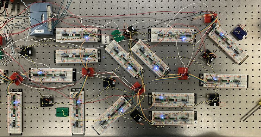
FIG. 2. Circuitry for Realization of Desynchronous Coupled
Learning. (A) Image of the entire 16-edge network. Edges with
FIG. 1. Coupled Learning is Successful Without a Global Clock LEDs on are active (updating) on this training step. (B) Diagram of
(A) Simulated 143 edge coupled learning network. (B) Test set the oscillator circuit in each edge in (A). A global bias voltage (red)
scaled error (error/error(t = 0)) curves averaged over 50 distinct 2- determines p. Each edge compares the bias against against a local
A B of training steps times
input 2-output regression tasks as a function oscillator signal (green) to determine if its resistance is updated.
Sources
update probability p. Colors denote differing values of p ranging
from 0.1 to 1. Error bars at the terminus of each curve denote range
of final error values for a given p when run for 20000 steps. This is a strikingly robust result, and signifies a substantive
Ground
potential simplification for an experimental coupled learning
Targets system, namely removing the global clock.
nodes are held at values closer to the desired outputs. When
η
1 this algorithm approaches gradient descent [19]. This
generates the ‘clamped’ response of the network.
143 Edge The voltage
Network EXPERIMENTAL (DISCRETE) COUPLED LEARNING
drop across each edge in the free ∆ViF and clamped ∆ViC states
then determine the change in resistance for that edge, given by We next test desynchronous updates in an experimental re-
γ alization of coupled learning. In recent work [18], coupled
δ Ri = 2 [∆ViC ]2 − [∆ViF ]2
(2) learning was first implemented in a physical system. In this
Ri
system, contrastive learning was performed in real time by
where Ri is the resistance of that edge and γ is a hyper pa- using two identical networks to access the free and clamped
rameter that determines the learning rate of the system. In states of the network simultaneously. The system was robust
effect, this learning rule lowers the power dissipation of the to real-world noise, and successfully trained itself to perform
clamped state relative to the free state, nudging the entire sys- a variety of tasks using a simplified version of the update rule
tem towards the (by definition) better clamped outputs. The that allowed only discrete values of R, specifically
system is then shown a new training example, and the process (
is repeated, iteratively improving the performance of the free +r0 if |∆ViC | + σ > |∆ViF |
δ Ri = (4)
state outputs. When a test set is given to the network to check −r0 otherwise.
its performance (by applying the input voltages appropriately)
errors are calculated via the difference between the free state Note that we have explicitly added the measured bias of the
outputs and the desired outputs. A more detailed description comparators σ , which we find manifests as a random, uni-
of coupled learning is given in previous work [19]. formly distributed variable from 0 to 0.05V. Each edge in the
In this algorithm, it is implicitly assumed that all edges up- network performed this update individually, but did so all at
date at the same time. Here we relax this assumption, modi- once, synchronized by a global clock. Here, we implement
fying the learning rule (2) with a probabilistic element: this learning rule [31] but incorporate a probabilistic element,
( such that with probability p each edge updates according to
δ Ri with probability p Eq. (4) on a given training step. Thus, we are able to tune the
∆Ri (p) = (3)
0 otherwise system from entirely synchronous (p = 1) to entirely desyn-
chronous (p
1). We implement this functionality via a sep-
where 0 < p ≤ 1 is the update probability and p = 1 recovers arate circuit housed on each edge of the network, shown in
synchronized coupled learning. This change, especially for Fig. 2(A), that, when triggered, compares an oscillating volt-
low p, fundamentally changes how the system updates. In- age signal to a global ‘bias’ voltage, as shown in Fig. 2(B).
dividual edges may spend long periods entirely static, while The components (comparators, capacitors, and resistors) used
the system evolves around them, completely ignoring large in each implementation of the oscillator vary slightly, chang-
changes along the way; that is, learning is desynchronized. ing the period, and thus the oscillating signals on each edge
In simulation, we find that desynchronization does not ham- rapidly desynchronize. Thus, by changing the bias value, we
per the learning process. In fact, the error as a function of can select p for our experimental system.
training steps times p consistently collapses for all values of As with the continuous version of coupled learning, desyn-
p for a variety of tasks and networks, as shown for a typical chronization does not prohibit the discrete, experimental sys-
example in Fig. 1. This collapse occurs regardless of choice of tem from learning. In fact, desynchronized learning performs
hyper parameters η (nudge amplitude) and γ (learning rate). better on average than synchronous learning for allosteric
3

                                                                         Thus we have, as before
                                A           D
                                                                                              (
                                                                                                 δ Ri   with probability p
                                                                                    ∆Ri (p) =                                        (5)
                                                                                                  0     otherwise
         B
                                                                         The addition of σ leads to a tendency for the resistor values
                                                                         to drift upwards, just like in the experiment, finding lower
                                                                         power solutions, and putting the resistors in a regime where
                                                                         they can take smaller steps relative to their magnitude. From
                                                                         simulations of a 143-edge discrete network, we find that as
                                C                                  E     allostery task complexity (number of targets and sources) in-
                                                                         creases, the beneficial effects of desynchronous learning di-
                                                                         minish, as shown in Fig. 3(D). More complex tasks require
                                                                         more desynchronous (lower p) learning to confer an advan-
                                                                         tage over synchronous learning. For tasks with enough tar-
                                                                         gets, moderately desynchronous learning yields indistinguish-
                                                                         able error from synchronous learning, as shown by the overlap
                                                                         of the blue and black curves on the right of Fig. 3(D).
FIG. 3. Desynchronization Improves Discrete Network Solutions               Unlike the experimental 16 edge network, desynchroniza-
in Experiment and Simulation. (A) Scaled error (error/error(t = 0))      tion does improve the error for our simulated 143-edge learn-
vs training steps scaled by update probability p in experiment for an    ing a two-source two-target regression task, as shown in
allosteric task. One typical raw (faded) and smoothed (color) curve      Fig. 3(E). We believe that for such a task, our 16-edge ex-
is shown for each of the three values of p. (B) Three resistor values    perimental network is in the ‘too-complex’ regime, whereas
vs training steps scaled by update probability from the experiments      our simulated 143-edge network is not, and therefore shows a
shown in (A). (C) Scaled error at the end of training averaged over      monotonic trend in final error with p.
25 allosteric tasks as a function of p. (D) Scaled error at the end of      Linear tasks like allostery and linear regression do not have
training averaged over 20 allosteric tasks as a function of number of    local minima [32] when the resistors are free to change con-
targets. Each task has an equal number of sources, and half as many
                                                                         tinuously. However, the discretization of resistor space creates
ground nodes as targets. Note the collapse of curves of varying p
as the task complexity grows. (E) Scaled test set error at the end of    many local minima, trapping the synchronous solution and
training in simulation averaged over 10 regression tasks. In (D) and     preventing it from finding a global optimum. As p decreases,
(E) the same 143 edge simulated network from Fig. 1(A) is used with      solutions increasingly drift from those found for synchronous
the discrete update rule (Eq. 5).                                        learning, as shown in Fig. 3F. These behaviors suggest that
                                                                         desynchronization aids in exploring an under-constrained re-
                                                                         sistance space, and escaping local minima, much like stochas-
                                                                         tic gradient descent in machine learning.
(fixed input and output) tasks, as apparent in even typical
error curves as shown in Fig. 3(A). Why does this stochas-
ticity improve results only when using the discrete learning              COMPARISON TO STOCHASTIC GRADIENT DESCENT
rule? Randomness allows the network to explore resistance
space. Edges continually evolve when p < 1 (desynchronous),                 In computational machine learning, artificial neural net-
whereas for p = 1 (synchronous), the system may find a local             works can be trained using batch gradient descent. In this
minimum and remain there indefinitely, as shown by the flat              algorithm, the entire set of training data is run through the
black resistor traces in Fig. 3(B). The ability to escape min-           network, and a global gradient is taken with respect to each
ima improves as the network becomes more desynchronized,                 weight in the network, averaged over the training set. The
leading to improved final error as p decreases for allosteric            weights are then modified based on this gradient until a local
tasks in experiment, as shown in Fig. 3(C). As tasks become              minimum is found. In practice, this method is inefficient at
more difficult, the beneficial effects of desynchronization are          best and intractable at worst [33]. A typical modification to
diminished. For a two-target, two-source regression task, our            this algorithm is known as stochastic gradient descent (SGD),
16-edge experimental network shows no benefit from desyn-                where instead of the entire training set, a randomly selected
chronization. However, as we now show in simulation, in-                 subset of training examples (mini-batch) is used to calcu-
creasing the size of the network brings learning back into a             late the gradient at each training step [12]. This effectively
regime where desynchronization confers an advantage.                     adds noise to the gradient calculation, speeds processing, and
   To test the advantages of desynchronous learning for fu-              boosts overall performance by allowing the system to contin-
ture larger realizations, we perform a simulation tailored to            ually evolve, escaping from local minima in the global cost
match our experimental system but with more edges. We                    function. Stochastic gradient descent has been shown to im-
use the discrete update rule (Eq. 4 with probability p), limit           prove learning performance in different settings, specifically
our resistance values to 128 linearly spaced values and use              in obtaining lower generalization (test) errors compared to
σ = U[0, 0.05] V (uniformly sampled between 0 and 0.05 V).               full batch gradient descent. It is therefore argued that SGD
4
A B where N is the total number of edges. Note the similar form
to the second line of Eq. (7). With this definition, the analogy
of desynchronous coupled learning and SGD is clear, with the
edge update probability p playing the role of the batch fraction
b̄, and thus we expect similar results for the two methods. We
verify the analogy between desynchronous coupled learning
and SGD in simulation.
For simulations with the continuous learning rule, we ob-
serve no change in final error when learning is desynchro-
nized, consistent with this picture, as there are no local min-
ima to escape. However, the analogy between SGD and
FIG. 4. Desynchronous Solutions Drift from Synchronous Solu- desynchronization can still be explored by observing the so-
tions. (A) Distance in continuous resistor space from synchronized, lutions in resistor space. As a base case, we simulate a
full-batched solution as a function of 1 − p for a 16-edge simulated,
N = 16 edge network (the same structure as our experiment
continuous network. Note mini-batching and desynchronization gen-
erate the same power law, as does their combined effect. (B) Same
in Fig. 2(A)) using the original coupled learning rule (Eq. 2)
as (A) but with constant number of edges updating or batch size (or with a full batch to solve a regression task with B = 16 training
both) at each training step. examples. That is for a given edge i,
B B
performs implicit regularization during training, finding local γ
[∆ViCj ]2 − [∆ViFj ]2
∆Ri = ∑ ∆Ri j = ∑ R2 (9)
minima in the cost landscape that are more likely to generalize j=1 j=1 i
to unseen input examples [14].
This can be more clearly understood by describing training where j is the index of the training example, summed over all
of a neural network as gradient descent dynamics of the learn- B = 16 elements of the training set. This is an entirely deter-
ing degrees of freedom w (edge weights in a neural network) ministic algorithm, given initial conditions of Ri , and thus a
with an additional diffusion term, following Chaudhari et al. good basis for comparison. Then we compare two forms of
[14]. We define b̄ as the fraction of training data points used stochasticity, randomly choosing edges (desynchronization)
in a mini-batch. Full-batch (b = 1) training simply minimizes and randomly choosing training examples (SGD). With prob-
the cost function C(w), and thus the dynamics may be written ability p we update edges (i), and with probability b we in-
as clude each training example in the sum ( j). For b = 1 we
use a full batch, and for p = 1 we update every edge syn-
γ −1 d~w(t) = −~∇wC(w)dt (6) chronously. Coupled learning as described in previous work
which yields solutions wb̄=1 that are minima of the cost func- [18, 19] used p = 1 and b
1 (a single training data point
tion. When mini-batching, an additional diffusion term is at a time). Decreasing p (desynchronizing) and decreasing
added to the dynamics, b (stochastic mini-batching) do not meaningfully change the
final error of the network’s solutions in continuous coupled
q learning, but do find different solutions than the full-batch
synchronous case. In fact, we find they have the same rela-
γ −1 d~w(t) = −~∇wC(w)dt + ~ (t)
2γ(b̄B)−1 D(w)dW
tionships to the fully deterministic solutions,
(7)
D(w) = [B−1 ∑ ~∇wCi ⊗ ~∇wCi ] − ~∇wC ⊗ ~∇wC
i
b = 1 : L2 ~R(p = 1), ~R(p) ∼ (1 − p)2/3 (10)
where the diffusion matrix D(w) is defined by outer prod-
ucts of the individual training example gradients, B is the total
number of training examples, and dW is a Wiener process.
These dynamics converge to critical points wb̄ that are dif- p = 1 : L2 ~R(b = 1), ~R(b) ∼ (1 − b)2/3 (11)
ferent from the minima of the cost function, wb̄=1 , by a factor
that scales with the fraction of data points not included in each Enforcing p = b also gives the same power law, all seen
batch (1 − b̄). This difference is the hallmark of regulariza- in Fig. 4(A). We may also enforce a randomly selected but
tion, in this case performed implicitly by SGD. consistent fraction of edges ( p̄) or of the training set (b̄) to
In coupled learning, the desynchronization of edge updates be updated/included for each training step. This is the stan-
is expected to yield a similar effect. Instead of having different dard means of mini-batching in SGD, as mentioned previ-
training examples, learning stochastically uses the gradient at ously. We find similar parallels between asynchronous and
independent edges. Therefore we can define an effective dif- mini-batched learning in this condition, as seen in Fig. 4(B).
fusion matrix for desynchronous coupled learning by The overall multiplicative factor separating the data can be ex-
plained by SGD and the desynchronous learning rule having a
γ 2 De f f (R) = [N −1 ∑ ∆Ri ⊗ ∆Ri ] − ∆~R ⊗ ∆~R different effective learning rate. Matching these effective rates
(8) collapses all data in Fig. 4(A) and (B).
i5
DISCUSSION opens the door for learning with new types of systems, ones
that cannot be synchronized such as elements updating out of
equilibrium [34], via thermal noise [29] or other stochastic
In this work we have demonstrated the feasibility of learn- processes.
ing without a global clock in a physics-based learning net- In discrete-valued coupled learning, mini-batching alone
work, both with a continuous state space of solutions and a (the standard in Coupled Learning) gives inferior results to
discrete one, in simulation and experiment. In all cases desyn- mini-batching plus asynchronous updates. This suggests that
chronizing the learning process does not hamper the ability in other learning problems with many local minima, includ-
of the system to learn, and in the discrete resistor space with ing in artificial neural networks, asynchronous updates could
many local minima, actually improves learning outcomes. We benefit the learning process. While we are not aware of
have shown that this improvement comes from a behavior this desynchronization algorithm used in such a way, similar
analogous to stochastic gradient descent, namely that injecting methods such as dropout [35] have been shown to be benefi-
noise into the learning process allows the system to escape lo- cial in improving generalizability of solutions [36], similar to
cal minima and find better overall solutions. Finally, we have stochastic gradient descent. True desynchronization would be
strengthened this analogy by showing that mini-batching and extremely inefficient in such a system, as then the entire gradi-
desynchronization produce the same scaling of distance in so- ent calculation is necessary for a single edge update. However,
lution space compared to a fully deterministic (full batch, syn- we have shown that benefits can be accrued by only moderate
chronous) algorithm. desynchronization, e.g. 80% update probability, which slows
the learning process proportionately. The true test of the use-
The freedom to avoid a global clock is an important step to- fulness of this algorithm will be in larger, nonlinear networks
wards total decentralization of the learning process in a phys- solving complex problems with many minima. This is a sub-
ical system; it is necessary to make a learning material. In ject for future work.
this and previous [18] work, the experimental system is still
run via a global clock, and thus requires a one bit communi-
cation with every edge to trigger resistor updates. However, ACKNOWLEDGMENTS
the success of all values of p demonstrates that edges with en-
tirely self-triggered updates would function well. For a larger, Thanks to Marc Miskin for insightful discussions, including
less precise, tighter packed, or three dimensional learning sys- on circuit design. This work was supported by the National
tems, removing this connection to each edge may greatly sim- Science Foundation via the UPenn MRSEC/DMR-1720530
plify construction. Furthermore, allowing desynchronization (S.D. and D.J.D.) and DMR-2005749 (M.S. and A.J.L.).
[1] N. C. Keim and S. R. Nagel, “Generic transient memory forma- 436–444, number: 7553 Publisher: Nature Publishing Group.
tion in disordered systems with noise,” 107, 010603, publisher: [11] P. Mehta, M. Bukov, C.-H. Wang, A. G. Day, C. Richardson,
American Physical Society. C. K. Fisher, and D. J. Schwab, “A high-bias, low-variance
[2] J. D. Paulsen, N. C. Keim, and S. R. Nagel, “Multiple tran- introduction to machine learning for physicists,” 810, 1–124.
sient memories in experiments on sheared non-brownian sus- [12] S. Ruder, “An overview of gradient descent optimization algo-
pensions,” 113, 068301, publisher: American Physical Society. rithms,” 1609.04747.
[3] N. C. Keim, J. D. Paulsen, Z. Zeravcic, S. Sastry, and S. R. [13] N. S. Keskar and R. Socher, “Improving generalization perfor-
Nagel, “Memory formation in matter,” 91, 035002, publisher: mance by switching from adam to SGD,” 1712.07628.
American Physical Society. [14] P. Chaudhari and S. Soatto, “Stochastic gradient descent per-
[4] R. G. Crowder, Principles of Learning and Memory: Clas- forms variational inference, converges to limit cycles for deep
sic Edition (Psychology Press) google-Books-ID: zWuL- networks,” in 2018 Information Theory and Applications Work-
BQAAQBAJ. shop (ITA) (IEEE) pp. 1–10.
[5] J. R. Anderson, Learning and memory: An integrated approach, [15] S. L. Smith, B. Dherin, D. G. T. Barrett, and S. De, “On the
2nd ed, Learning and memory: An integrated approach, 2nd ed origin of implicit regularization in stochastic gradient descent,”
(John Wiley & Sons Inc) pages: xviii, 487. , 14.
[6] J. J. Hopfield, “Neural networks and physical systems with [16] Y. Feng and Y. Tu, “The inverse variance–flatness relation in
emergent collective computational abilities.” 79, 2554–2558. stochastic gradient descent is critical for finding flat minima,”
[7] R. McEliece, E. Posner, E. Rodemich, and S. Venkatesh, “The 118, 10.1073/pnas.2015617118, publisher: National Academy
capacity of the hopfield associative memory,” 33, 461–482, of Sciences Section: Physical Sciences.
conference Name: IEEE Transactions on Information Theory. [17] M. Ruiz-Garcia, G. Zhang, S. S. Schoenholz, and A. J. Liu,
[8] J. W. Rocks, N. Pashine, I. Bischofberger, C. P. Goodrich, A. J. “Tilting the playing field: Dynamical loss functions for ma-
Liu, and S. R. Nagel, “Designing allostery-inspired response in chine learning,” 2102.03793.
mechanical networks,” 114, 2520–2525. [18] S. Dillavou, M. Stern, A. J. Liu, and D. J. Durian, “Demonstra-
[9] M. Stern, M. B. Pinson, and A. Murugan, “Continual learning tion of decentralized, physics-driven learning,” 2108.00275.
of multiple memories in mechanical networks,” 10, 031044, [19] M. Stern, D. Hexner, J. W. Rocks, and A. J. Liu, “Supervised
publisher: American Physical Society. learning in physical networks: From machine learning to learn-
[10] Y. LeCun, Y. Bengio, and G. Hinton, “Deep learning,” 521, ing machines,” 11, 021045 (), publisher: American Physical6
Society. lisher: Nature Publishing Group.
[20] M. Stern, V. Jayaram, and A. Murugan, “Shaping the topology [29] D. Kappel, S. Habenschuss, R. Legenstein, and W. Maass,
of folding pathways in mechanical systems,” 9, 4303. “Network plasticity as bayesian inference,” 11, e1004485.
[21] M. Stern, C. Arinze, L. Perez, S. E. Palmer, and A. Murugan, [30] D. Dolev, J. Y. Halpern, and H. R. Strong, “On the possibil-
“Supervised learning through physical changes in a mechanical ity and impossibility of achieving clock synchronization,” 32,
system,” 117, 14843–14850 (). 230–250.
[22] N. Pashine, “Local rules for fabricating allosteric networks,” 5, [31] Specifically in this work we use comparators and an XOR gate
065607, publisher: American Physical Society. to evaluate XOR[ (∆ViC > ∆ViF ) , (∆ViC + ∆ViC > 0)].
[23] N. Pashine, D. Hexner, A. J. Liu, and S. R. Nagel, “Directed [32] A. C. Rencher and G. B. Schaalje, Linear models in statistics,
aging, memory, and nature’s greed,” 5, eaax4215. 2nd ed. (Wiley-Interscience) OCLC: ocn144331522.
[24] D. Hexner, N. Pashine, A. J. Liu, and S. R. Nagel, “Effect of [33] N. Golmant, N. Vemuri, Z. Yao, V. Feinberg, A. Gholami,
directed aging on nonlinear elasticity and memory formation in K. Rothauge, M. W. Mahoney, and J. Gonzalez, “On the com-
a material,” 2, 043231. putational inefficiency of large batch sizes for stochastic gradi-
[25] D. Hexner, A. J. Liu, and S. R. Nagel, “Periodic training of ent descent,” 1811.12941.
creeping solids,” 117, 31690–31695. [34] M. Stern, S. Dillavou, M. Z. Miskin, D. J. Durian, and
[26] B. Scellier and Y. Bengio, “Equilibrium propagation: Bridging A. J. Liu, “Physical learning beyond the quasistatic limit,” (),
the gap between energy-based models and backpropagation,” 2112.11399.
11, 10.3389/fncom.2017.00024, publisher: Frontiers. [35] In dropout, some fraction of edges in a layer of a neural net-
[27] J. Kendall, R. Pantone, K. Manickavasagam, Y. Bengio, and work are removed for that training step. This is distinct from
B. Scellier, “Training end-to-end analog neural networks with asynchronous learning, where all edges are present for calcu-
equilibrium propagation,” 2006.01981. lating the outputs, but some simply do not update.
[28] L. F. Abbott and S. B. Nelson, “Synaptic plasticity: taming [36] N. Srivastava, G. Hinton, A. Krizhevsky, I. Sutskever, and
the beast,” 3, 1178–1183, bandiera_abtest: a Cg_type: Nature R. Salakhutdinov, “Dropout: A simple way to prevent neural
Research Journals Number: 11 Primary_atype: Reviews Pub- networks from overfitting,” 15, 1929–1958.You can also read