Linking aquatic biodiversity loss to animal product consumption: A review
←
→
Page content transcription
If your browser does not render page correctly, please read the page content below
MSc Biological Sciences
                        Freshwater and Marine Biology

                                Literature Review

          Linking aquatic biodiversity loss to animal product
                       consumption: A review

                                         by

                               Michelle Pena-Ortiz
                                   11567791

                                      July 2021
                                       12 ETCS

                 Supervisor & Assessor: Dr. Brian Machovina 1
                     Examiner: Dr. Harm van der Geest 2

      1 College of Arts, Sciences, and Education – Florida International University
2
    Institute for Biodiversity and Ecosystem Dynamics - Universiteit van Amsterdam

                                                                                  1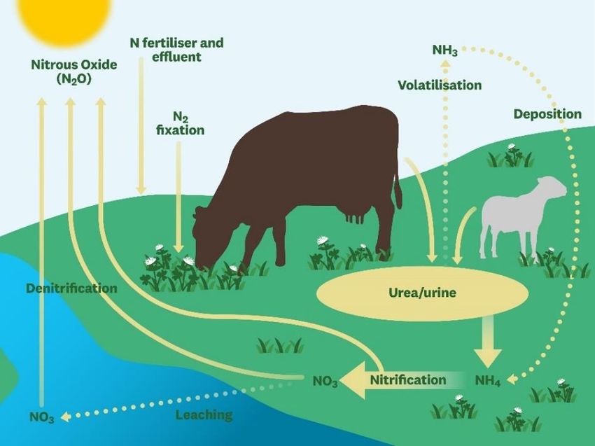
Table of Contents
Abstract ........................................................................................................................................................ 3
1. Introduction .............................................................................................................................................. 5
2. Methodology ............................................................................................................................................ 8
3. Pressures................................................................................................................................................... 8
   3.1. Habitat alteration ...............................................................................................................................................9
       3.1.1. Riparian zones ...........................................................................................................................................10
       3.1.2. Channelization ..........................................................................................................................................12
       3.1.3. Water extraction .......................................................................................................................................13
   3.2. Climate change .................................................................................................................................................13
       3.2.1. CH4 ............................................................................................................................................................14
       3.2.2. N2O ............................................................................................................................................................16
       3.2.3. CO2 ............................................................................................................................................................17
   3.3. Pollution ...........................................................................................................................................................19
       3.3.1. Nutrients ...................................................................................................................................................20
       3.3.2. Sediment ...................................................................................................................................................21
       3.3.3. Antibiotics .................................................................................................................................................22
       3.3.4. Estrogenic compounds ..............................................................................................................................23
   3.4. Alien species .....................................................................................................................................................23
   3.5. Overexploitation...............................................................................................................................................24
4. State ........................................................................................................................................................ 26
   4.1. Habitat alteration .............................................................................................................................................26
   4.2. Climate change .................................................................................................................................................28
       4.2.1. Effects of increased in-water temperatures on aquatic biodiversity ........................................................28
       4.2.1. Effects of altered precipitation on aquatic biodiversity ............................................................................30
   4.3. Pollution ...........................................................................................................................................................31
   4.4. Alien species .....................................................................................................................................................34
   4.5. Overexploitation...............................................................................................................................................36
   4.6. Multi-stress ......................................................................................................................................................37
5. Potential responses ................................................................................................................................ 38
   5.1. Production ........................................................................................................................................................38
   5.2. Consumption ....................................................................................................................................................40
5. Conclusions ............................................................................................................................................. 43
Literature cited ........................................................................................................................................... 44

                                                                                                                                                                             2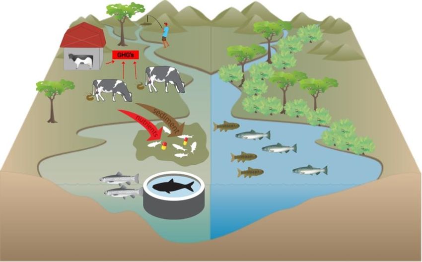
Abstract
Animal agriculture, which accounts for 83% of global farmland, but produces only 18% of global
calories, is responsible for the majority of agriculture-related environmental degradation. The
pressures that animal product consumption place on the environment include habitat alteration,
climate change, pollution, invasive species introductions, and overharvesting of wild animals.
These pressures are the five main drivers of biodiversity loss and for most ecosystems, each
pressure is currently either constant or growing. It has recently been established that aquatic
(freshwater) ecosystems are particularly vulnerable to these pressures yet remain less studied
and less protected than terrestrial and marine ecosystems. Although it is well known that animal
product consumption is a leading driver of the aforementioned pressures, and aquatic
biodiversity is declining as a result of these pressures, the link between animal product
consumption and aquatic biodiversity loss has not been thoroughly explored. Therefore, the aim
of this literature review was to evaluate how animal product consumption contributes to aquatic
biodiversity loss by analyzing the contribution of animal agriculture to the five main drivers of
biodiversity loss and investigating how aquatic biodiversity is affected by each of these drivers.
Moreover, this review proposed potential responses that would help mitigate the effect of these
pressures on aquatic biodiversity. This review found that there is a strong link between animal
product consumption and aquatic biodiversity loss, and that animal agriculture is likely a primary
driver of aquatic biodiversity loss. Research on potential responses demonstrated that
decreasing or eliminating consumption of animal products was the most impactful strategy for
alleviating pressures placed on aquatic biodiversity when compared to supply-side interventions,
such as increasing efficiency. More specifically, global adoption of plant-based diets could reduce
agricultural land-use by 76%, which is equivalent to an area more than three times the size of the
United States, including Alaska, Hawaii, and Puerto Rico, as well as result in 358-743 GtCO2
removal via carbon sequestrations through restoration, which is roughly equivalent to the past 9
to 16 years of fossil fuel emissions.

Keywords: animal products, agriculture, aquatic biodiversity loss, meat consumption, plant-
based diets

                                                                                                 3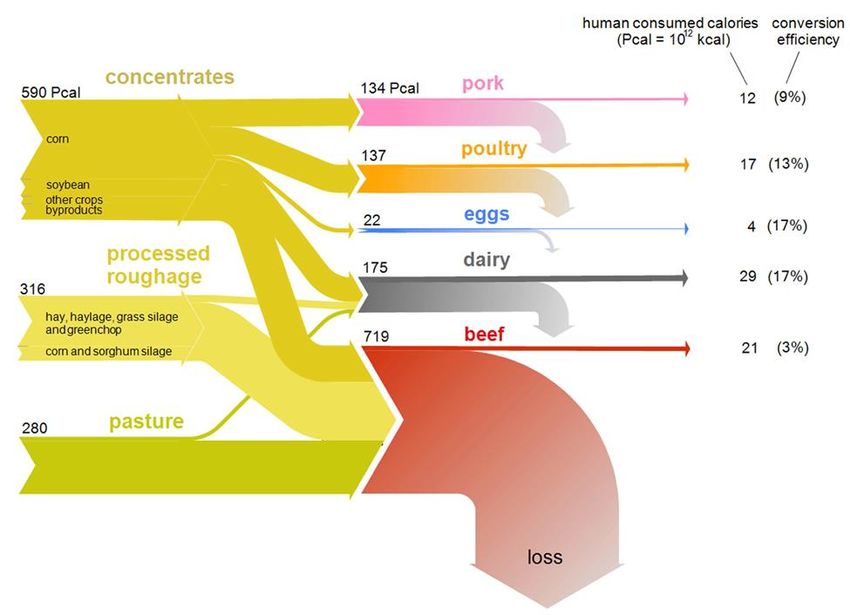
5.

                         2.

                              3.

          1.

                    4.

Figure 1. Graphical abstract depicting the five pressures of animal product consumption on
aquatic biodiversity in a river (left), and aquatic biodiversity in the absence of these pressures,
for reference (right). Depictions of pressures are numbered as follows: (1) Habitat alteration i.e.,
degraded riparian buffer, (2) Climate change due to release of GHGs, (3) Pollution from
nutrients, sediment, and pharmaceuticals, (4) Alien species escaping from aquaculture, and (5)
Overconsumption of wild freshwater animals.

                                                                                                   4
1. Introduction
It is widely known that global agriculture is a predominant driver of various forms of
environmental degradation (Campbell et al., 2017; Foley et al., 2005; Steinfeld et al., 2006).
Animal agriculture, which accounts for 83% of global farmland, but produces only 18% of global
calories (Poore & Nemecek, 2018), is responsible for the majority of agriculture-related
environmental degradation (Clark & Tilman, 2017; Machovina et al., 2015; Springmann et al.,
2018; Willet et al., 2019). In addition to animal agriculture, the direct consumption of animals via
harvesting (e.g., hunting and fishing) also contributes to environmental degradation by altering
trophic interactions and decreasing biodiversity (Machovina et al., 2015). Despite the urgent
need to curtail the pressures that animal consumption places on the environment, it is estimated
that the demand for meat and dairy will increase by 68% and 57%, respectively, by 2030 (McLeod,
2011).

Myriad studies have demonstrated that animal products with the lowest impact on the
environment, such as poultry and eggs, still exceed average environmental impacts of crops
across indicators such as greenhouse gas (GHG) emissions, land use change, nutrient pollution,
and energy use (Clark & Tilman, 2017; Poore & Nemecek, 2018; Ripple et al., 2014; Swain et al.,
2018; Willett et al., 2019). Animal products most commonly include beef, pork, chicken, fish,
dairy, and eggs, which are produced in conventional systems such as Confined Animal Feeding
Operations (CAFO), pasture or free-range systems, aquaculture ponds, and/or wild harvest. The
key reason for the significantly larger environmental impacts of animal products, compared to
crop products, is the inherent inefficiency of energy transfer between trophic levels when
converting plant calories into animal calories (Cassidy et al., 2013; Swain et al., 2018). Therefore,
when addressing animal product consumption’s effects on the environment, it is important to
consider not only the resources utilized directly by the animals, but the feed crops as well. Studies
show that the ratio of animal product calories to feed calories is on average 7-10%, yet conversion
efficiency is dependent on the animal product (Godfray et al., 2010; Sherpon et al., 2016).
Sherpon et al. (2016) found that conversion efficiency between crop and animal products in the

                                                                                                   5
US can ranges from 3% to 17%, suggesting that using edible crops to feed animals is an inefficient
way to provide food for humans (Figure 2).

Figure 2. A Sankey flow diagram of the US feed -to-food caloric flux from the three feed classes
(left) into edible animal products (right). On the right, parenthetical percentages are the food -
out/feed-in caloric conversion efficiencies of individual livestock categories. From Sherpon et al.
(2016)

The pressures that animal product consumption place on the environment include habitat
alteration, climate change, pollution, invasive species introductions, and overharvesting of wild
animals (Allan et al., 2005; Clark & Tilman, 2017; De Silva et al., 2009; Poore & Nemecek, 2018;
Ripple et al., 2014; Swain et al., 2018; Willett et al., 2019). According to the Millennium Ecosystem
Assessment (2005), these pressures are the 5 main drivers of biodiversity loss, and for most
ecosystems, each pressure is currently either constant or growing. This suggests that animal
product consumption is a major driver of biodiversity loss, and potentially the leading cause of
modern species extinctions (Machovina et al., 2015). It has recently been established that aquatic
(freshwater) ecosystems are particularly vulnerable to these pressures yet remain less studied
and less protected than terrestrial and marine ecosystems (MEA, 2005; WWF, 2020). More
                                                                                                   6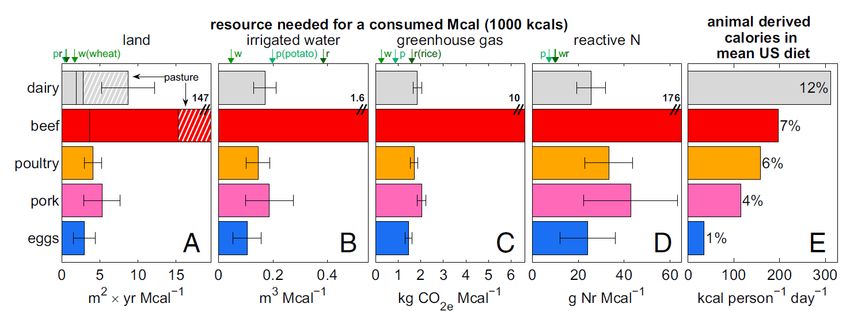
specifically, the pressures of habitat alteration, climate change, pollution, and alien species
introductions have been found to be rapidly increasing and have a “very high” effect on
biodiversity in freshwater ecosystems, while overharvesting remains stable, and has a
“moderate” impact on freshwater biodiversity (MEA, 2005). Aquatic species populations are
declining at a rate of 4% a year, resulting in a total loss of 83% since 1970, according to an analysis
of 3,741 monitored populations in the Freshwater Living Planet Index (WWF, 2020). Other studies
have found that almost one in three freshwater species are at risk of extinction, with all
taxonomic groups showing a higher risk of extinction than terrestrial ecosystems (Collen et al.,
2014). Although it is well known that animal product consumption is a leading driver of the
aforementioned pressures, and aquatic biodiversity is declining as a result of these pressures, the
link between animal product consumption and aquatic biodiversity loss has not been thoroughly
explored.

Therefore, the aim of this literature review was to evaluate how animal product consumption
contributes to aquatic biodiversity loss by analyzing the contribution of animal agriculture to the
five main drivers of biodiversity loss and investigating how aquatic biodiversity is affected by each
of these drivers. Analyzing the effects of animal product consumption on aquatic biodiversity loss
should give new insight into potential responses societies can adopt to mitigate this pressing
environmental issue. The following questions have been raised to address the aim of this review:
       1. What pressures are being placed on aquatic biodiversity as a result of animal product
       consumption?
       2. What is the state of aquatic biodiversity as a result of these pressures?
       3. What are potential responses to mitigate aquatic biodiversity loss driven by animal
       product consumption?

To answer these questions, this literature review will remain specific to the United States (US), a
megadiverse country, where meat consumption is three times greater than the global average
(Poore & Nemecek, 2018). The structure of this review is loosely modeled after the FAO’s
pressure-state-response (PSR) framework (OECD, 1999).

                                                                                                     7
2. Methodology
This literature review focused on acquiring available data that demonstrated the pressures that
animal agriculture places on aquatic biodiversity, data that showed how aquatic biodiversity is
affected by these pressures, and lastly, data that illustrated potential solutions to combat these
pressures and improve the current state of aquatic biodiversity as a result of these pressures.
Literature was primarily collected using academic search engines GoogleScholar, ScienceDirect,
and University of Amsterdam’s publication database CataloguePlus. Relevant literature was
found using key terms “animal agriculture”, “livestock grazing”, “USA CAFOs”, “livestock nutrient
runoff”, “plant-based diets”, “overfishing freshwater US”, “antibiotics CAFO”, “estrogenic
pollution livestock”, “aquatic invertebrate livestock”, and “climate change”. National agriculture
statistics were retrieved by accessing governmental databases of the Environmental Protection
Agency (EPA) and United States Department of Agriculture (USDA). This review aimed to
synthesize existing scientific literature and draw conclusions based on data published by other
authors, rather than contribute new findings. This review also offered conclusions based on
available data and provided insight into knowledge gaps that could be addressed in future
studies.
3. Pressures
The pressures that animal product consumption place on the aquatic biodiversity include habitat
alteration, climate change, pollution, alien species introductions, and overexploitation of wild
animals. The following sections will focus on the contributions of animal agriculture to each of
these pressures. It is important to note that numerous studies demonstrate that animal products
differ in their contribution to these pressures.
8Figure 3. Overview of environmental pressures of animal agriculture. (A–D) Environmental
performance of the key livestock categories in the US diet, jointly accounting for >96% of animal -
based calories. Authors report performance in resources required for producing a consumed
Mcal (1 Mcal = 1000 kcal, roughly half a person’s mean daily caloric needs). For comparison,
resource demands of staple plants potatoes (denoted p), rice (r), and wheat (w) are denoted by
arrows above A–D. E displays actual US consumption of animal-based calories. Values to the right
of the bars denote categories’ percentages in the mean US diet. The demands of beef are larger
than the figure scale and are thus written explicitly next to the red bars representing beef. Error
(uncertainty) bars in dicate SD. In A, for beef and dairy, demand for pastureland is marked with
white hatching, and a vertical line separates demand for cropland (to the left), and processed
roughage land (to the right). From Eshel et al. (2014).
3.1. Habitat alteration
Animal product production (including feed crop production) takes up approximately 43% of all
ice and desert-free land on earth, making it the single largest anthropogenic land use on the
planet (Poore & Nemecek, 2018). In the US, grazing land for cattle accounted for approximately
35% - or 798 million acres - of total land area in 2012, making it the single largest land use type
in the country (Bigelow & Borchers, 2017). Moreover, cropland accounts for approximately 17%
- or 392 million acres – of total land in the US (Bigelow & Borchers, 2017), 40% of which is
dedicated to animal feed (Eshel et al., 2014). Pasture-raised cattle typically account for the most
terrestrial land use in the US (Figure 3), whereas in pig and chicken systems, nearly all associated
land use is for feed crop production (de Vries & de Boer, 2010). Terrestrial pasturelands and feed
croplands alter adjacent aquatic habitats by degrading riparian zones that are important for
regulating shade, temperature, and organic matter inputs (Belsky et al., 1999; Goss & Roper,
2018; Jones et al., 2001; Wetzel, 2001). Aside from terrestrial land use change, animal product
9production directly alters aquatic ecosystems via drainage alteration and/or channelization of
streams and rivers that is carried out to facilitate feed crop yields (Lau et al., 2006; Raborn &
Schramm, 2003; Sullivan et al., 2004). Water extraction for feed crops and pasture lands modifies
aquatic ecosystems by reducing flow (Richter et al., 2020).
3.1.1. Riparian zones
Riparian zones are considered the interface between terrestrial and aquatic ecosystems, and
provide aquatic ecosystems with shade, allochthonous material (food), and habitat, while at the
same time maintaining bank stability. Livestock grazing has been shown to be a key factor in the
continued degradation of riparian zones (Batchelor et al., 2014; Behnke, 1978; Platts, 1982),
particularly in the western US (Belsky et al., 1999; USDI, 1994). According to Armour et al.,
(1994), grazing by livestock has damaged 50% of riparian zones in arid regions of the western US,
whereas US Department of Interior (1994) found that livestock grazing had damaged 80% of
streams and riparian zones in the arid west. Myriad studies demonstrate that cattle access to
streams results in loss of bank vegetation and trampling of streambanks (Batchelor et al., 2014;
Bryant et al. 1972; Goss & Roper, 2018; Kauffman et al., 2004; Trimble & Mendel, 1995), which
degrades stream water quality and in-stream habitats (Armour et al., 1994; Kauffman & Krueger,
1984).
Grazing cattle decrease riparian vegetative biomass and therefore overhead cover, as well as
alter vegetative composition and diversity, which has profound impacts on aquatic habitats
(Bryant et al. 1972, Chapman & Knudsen 1980; Evans & Krebs 1977; Kauffman et al., 2004; Knoph
& Cannon 1982). In a study done on Rock Creek in Montana, Meehan & Platts (1978) observed
that streamside riparian cover was 76.4% greater in ungrazed areas compared to grazed areas.
Loss of riparian vegetative cover has been shown to increase average in-stream water
temperatures, as well as decrease allochthonous inputs (Delong & Brusven, 1994; Sizer, 1992;
Pozo et al., 1997; Jones et al., 2001; Wetzel, 2001). Previous studies have observed that lack of
vegetative covering in cattle grazing areas can increase average in-stream water temperatures
by 5-7°C (Nussle et al., 2015; Zoellick, 2004). Van Velson (1979) discovered that average water
10temperatures decreased from 24°C to 22°C one year after cattle exclusion from a creek in
Nebraska. Moreover, decreases in allochthonous material associated with lack of riparian cover
decreases C/N ratios in lakes and streams, since the supply of C is degraded. Higher C/N ratios in
aquatic habitats are associated with higher food web stability (Lu et al., 2014; Rooney & McCann,
2012), and as C/N ratios decrease, there is a shift in detrital processing and nutrient levels (Delong
& Brusven, 1994; Sizer, 1992; Pozo et al., 1997). Associated changes in detrital processing in
upstream reaches of a stream could affect downstream trophic dynamics via reduction of
transported fine particulate organic matter (Cuffney et al., 1990).
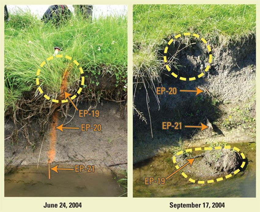
Trampling of streambanks by cattle causes bank slumping (Figure 4), which eventually leads to
stream channels becoming wider and shallower (Batchelor et al., 2014; Goss & Roper, 2018;
Herbst et al., 2012; Knapp & Matthews, 1996; Trimble & Mendel, 1995). Reductions in-stream
width/depth ratio create a larger stream surface area that is exposed to solar radiation, thus
further exacerbating the increase in average stream water temperature that occurs from loss of
vegetative overhead cover (Herbst et al., 2012; Kauffman et al., 1983). Additionally, trampling of
streambanks, coupled with the loss of riparian vegetation, results in decreased infiltration
potential of soil, leading to higher peak flows in streams (Behnke, 1978; Belsky et al., 1999).
Typically, water that percolates into the ground moves through sub-soil and seeps into stream
channels through the year, creating perennial flows. However, as cattle compact soil and degrade
vegetation, less rainwater infiltrates the soil and instead flows overland into streams, creating
peak flows (Belsky et al., 1999). Trimble & Mendel (1995) estimated that peak storm runoff from
a 120-hectare basin in Arizona would be 2-3 times higher when riparian areas were heavily grazed
compared to lightly grazed. High intensity flows in grazed areas further alter stream morphology
by incising and/or eroding stream banks, and deepening channels (Belsky et al., 1999; USDI,
1994). Furthermore, the interruption of perennial flows in riparian areas results in aquatic
ecosystems receiving less water during late-season flows (Kovalchik & Elmore, 1992; Li et al.,
1994; Ponce & Lindquist, 1990). Degradation of riparian zones also contributes to increased
sedimentation and nutrient loads in aquatic habitats, reviewed in later sections of this paper.
11Figure 4. Erosion pins (EP) record a bank failure due to cattle access . The numbers are obsolete
and refer to tables in Peppier & Fitzpatrick (2005) . The yellow dashes mark the riparian block
that failed. Image taken from Peppler & Fitzpatrick (2005) .
3.1.2. Channelization
Stream channelization is a common practice in US croplands, because it can reduce the risk of
crop loss from excess water stress and allows farmers more control over harvest conditions
(Blann et al., 2009; Spaling & Smit, 1995). Although most literature on this topic does not specify
these channelized regions as “feed crop agriculture”, it is important to discuss channelization in
relation to animal agriculture, as feed crops make up 40% of crop production in the US (Eshel et
al., 2014). For example, the Midwest produces 33% of the world’s corn (FAO, 2017), with most
of this corn being used as the main energy source in livestock feed (WAOB, 2020). Many of the
streams in agricultural regions of the Midwest have been exposed to severe and repeated
channelization (Edwards et al., 1984; Emerson, 1971). Channelization of streams negatively
12modifies crucial habitat parameters such as pool/glide quality, riffle/run quality, channel
morphology, and substrate (Lau et al., 2006; Raborn & Schramm, 2003; Sullivan et al., 2004).
Unchanneled streams harbor a variety of velocities, depths, widths, and substrates as a result of
natural stream meandering, producing well developed and interspersed riffle and pool habitats
(Aadland, 1993; Gorman & Karr, 1978; Scarnecchia, 1988). Channelization causes homogenous
stream width and depth, making it difficult to distinguish between riffle and pool habitats that
are important for aquatic biodiversity (Gorman & Karr, 1978; Smiley & Gillespie 2010).
3.1.3. Water extraction
Feed crop production requires approximately 45 billion m3 of water, totaling about 27% of the
total national irrigation use (Eshel et al., 2014). Almost 80% of irrigated feed crops are fed to beef
cattle, and approximately 15% are fed to dairy cattle, making cows the largest consumers of
irrigated feed crops in the US (Eshel et al., 2014; Richter et al., 2020) (Figure 3). According to
Richter et al., (2020), irrigation of cattle-feed crops is the single largest consumer at both regional
and national scales in the US, with 17 western states producing nearly all the feed crops that
require irrigation due to the arid nature of these ecosystems (Richter et al., 2020; Schaible &
Aillery, 2012). More specifically, cattle-feed irrigation is the leading driver of flow depletion in
one-third of all western US sub-watersheds, and more than one-quarter of western rivers in the
US are depleted by over 75% during summer months, with cattle-feed irrigation being the largest
water use in more than half of these rivers (Richter et al., 2020). River flow depletion due to
cattle-feed irrigation occurs when surface water is extracted, or shallow groundwater near rivers
is pumped. Water extraction has the potential to exacerbate other adverse anthropogenic
impacts on aquatic habitats such as water pollution, decreased oxygen levels, and opportunity
for alien species of fish to outcompete native species (Poff & Zimmerman, 2010; Richter et al.,
1997).
3.2. Climate change
Climate change is primarily caused by the release of greenhouse gases into the atmosphere (IPCC,
2013). Globally, livestock farming accounts for 14.5% (7.1 gigatons CO2-eq per annum) of total
13anthropogenic GHG emissions (Gerber et al., 2013) and is the primary anthropogenic source of
methane (CH4) and nitrous oxide (N2O) emissions, producing 44-50% and 53-60%, respectively
(Gerber et al., 2013; Smith et al., 2007). The global livestock sector’s emissions are comprised of
44% CH4, 29% N2O, and 27% CO2 (IPCC, 2007), with dairy and beef cattle contributing
approximately 65-77% of these emissions (Gerber et al., 2013; Herrero et al., 2013). Pigs,
chickens, and small ruminants contribute much less to emission levels, with each representing
between 7-10% of sector emissions (Gerber et al., 2013). In 2019, beef cattle accounted for 72%
of total national livestock CH4 (EPA, 2021). In the US, fertilizer application and manure
management make up a significant portion of national N 2O emissions, whereas crop feed
production, agricultural land use change, and crop feed transportation make up a significant
portion of national CO2 emissions (EPA, 2021). GHG emissions has resulted in an increase of 1°C
above pre-industrial levels (IPCC, 2013). This anthropogenic warming alters the water cycle, and
therefore, spatial and seasonal precipitation patterns (IPCC, 2013). This change in air
temperature has substantial impacts on aquatic ecosystems, including increasing in-stream water
temperatures and altering in precipitation patterns, which lead to periods of floods and drought
(Knouft & Ficklin, 2017).
3.2.1. CH4
Methane is estimated to have a global warming potential (GWP) of 28-36 CO2-eq over 100 years
(CO2 is used as a reference and therefore has a GWP of 1) and stays in the atmosphere for
approximately 10 years (EPA, 2021; IPCC, 2013). It is important to note that GWP calculations
differ. The EPA uses a 100-year GWP of 25 CO2-eq for the national GHG inventory, based on
calculations from the 2007 IPCC report (EPA, 2021; IPCC, 2007). The higher GWP of CH4 compared
to CO2 is attributed to the fact that CH4 absorbs considerably more energy and is a precursor to
ozone, which is another GHG (EPA, 2021; IPCC, 2013). In the US, animal agriculture is the largest
anthropogenic contributor of CH4, primarily via enteric fermentation and manure storage
systems.
14Enteric fermentation is responsible for most anthropogenic CH4 emissions in the US, representing
27.1% of total anthropogenic CH4 in 2019 (EPA, 2021). In ruminants (e.g., cows, goats), enteric
fermentation is the process of microbes decomposing and fermenting plant materials such as
starch, cellulose, and sugars in the digestive track or rumen. Enteric methane is a byproduct of
this process and is expelled from the animal via burping (Gerber et al., 2013; Ripple et al., 2014).
Nonruminant, or monogastric, animals such as pigs and chickens produce negligible enteric
methane emissions in comparison (Ripple et al., 2014). The large contribution of enteric
fermentation to national CH4 emission levels can be explained by the findings of Eshel et al.,
(2014), which show that dairy and beef are the two most consumed animal products in the US
(kcal/person/day), accounting for 12% and 7% of all consumed calories (Figure 3). In 2019, enteric
fermentation was responsible for emitting 178.6 million metric tons (MMT) CO2-eq, representing
an increase of 13.9 MMT CO2-eq. since 1990 (EPA, 2021). This increase in emissions from 1990
to 2019 follows the trend of increases in beef and dairy cow populations (EPA, 2021).
Manure management was the 4th largest contributor of anthropogenic CH4 in the US,
representing 9.5% of total CH4 emissions in 2019 (EPA, 2021). Manure that is handled as a liquid
or slurry is typically stored in an integral tank that is under a confinement facility or flushed into
an external anaerobic waste lagoon or pond (EPA 2020). The anaerobic decomposition that takes
place in these systems breaks down volatile solids in livestock manure, which produces CH4 (EPA,
2020; Gerber et al., 2013; Leytem et al., 2017). The EPA (2021) estimated that CH4 emissions from
livestock manure management were 62.4 MMT CO2-eq. in 2019, representing an increase of 25.3
MMT CO2-eq. since 1990, primarily due to increased concentrations of dairy and swine
production (EPA, 2021). In 2019, CH4 emissions from dairy cattle manure produced 32.0 MMT
CO2-eq, followed by swine manure, which produced 23.1 MMT CO2-eq. (EPA, 2021; Leytem et al.,
2017). Poultry and beef cattle manure produced 3.6 MMT CO2-eq and 3.4 MMT CO2-eq,
respectively, in 2019 (EPA, 2021). This large discrepancy in CH4 manure management emissions
is primarily due to the increased concentration of dairy cows and pigs in confinement facilities.
Despite the national dairy cow count decreasing since 1990, the industry has become more
15concentrated in certain states, resulting in higher density confinement facilities that utilize liquid-
based management systems to flush or store manure (EPA, 2021).
3.2.2. N2O
Nitrous oxide is estimated to have a GWP of 265-298 CO2-eq over 100 years and remains in the
atmosphere for more than 100 years, on average (IPCC, 2007; Steinfeld et al., 2006). The
significantly higher GWP of N2O compared to CO2 is attributed to the fact that it is significantly
more effective at absorbing thermal radiation and plays a role in degrading stratospheric ozone
(Poffenbarger et al., 2018). Nitrous oxide is primarily produced as an intermediary between
nitrification and denitrification, which are anthropogenically altered via agriculture (EPA, 2020;
EPA, 2021). The livestock sector in the US primarily contributes N2O through application of
manure on crops and pastures and manure management and storage (EPA, 2020; EPA, 2021).
Agricultural soil management is responsible for most anthropogenic N2O emissions in the US,
representing 75.4% of total anthropogenic N2O emissions, and 5.3% of total GHG emissions in
2019 (EPA, 2021). According to the EPA (2021), agricultural soil management activities include
application of synthetic and organic fertilizers, deposition of livestock manure, and growing N-
fixing plants; therefore, it is difficult to quantify the contribution of livestock to this value. Yet, it
is known that the fertilization of feed crops and deposition of manure on crops and pastures
generate substantial amounts of N2O emissions (Steinfeld et al., 2006; Gerber et al., 2013).
Nitrogen is an important macronutrient for plants that is used to improve crop yield; however,
plants often do not uptake all the reactive N available in fertilizers and manure. This results in
runoff of N, which eventually reacts with soil and produces N 2O as a byproduct (EPA, 2020).
Globally, livestock production and feed crop production produce 65% of N 2O emissions (EPA,
2020), although this number is difficult to discern in the US.
16Nitrous oxide can be produced
via microbial decomposition
of organic nitrogen in livestock
manure during management
and storage (EPA, 2021;
Gerber et al., 2013). The EPA
(2021) estimated that manure
management was the 4th
largest contributor of
anthropogenic N2O emissions,
representing 4.3% of total
emissions in 2019. These Figure 5. Nitrous oxide released via livestock manure. From
De Klein et al., (2008)
emissions are most likely to
occur in unpaved beef and dairy cow drylots since these sites are susceptible to nitrification and
denitrification processes, in which the byproduct is N2O (EPA, 2020) (Figure 5). In unpaved
feedlots, NH4 that is not lost to volatilization will be absorbed by the soil and be oxidized to NO 2
or NO3. The subsequent process of denitrification is dependent on on-site soil drainage – in poorly
drained soils, anaerobic conditions needed for denitrification will be more likely, and therefore,
will result in more N2O emissions (EPA, 2020). In 2019, N2O emissions from manure management
and storage were approximately 20 MMT CO2-eq, representing an increase of 5.6 MMT CO2-eq
since 1990, primarily due to the increase in specific livestock populations (EPA, 2021).
3.2.3. CO2
Carbon dioxide is considered the most prevailing GHG despite having the lowest radiative forcing,
because the vast majority of GHG emissions are CO2, and it has a longer atmospheric lifetime
(EPA, 2020; IPCC, 2007). CO2 has a GWP of 1 CO2-eq over 100 years, and anthropogenic emissions
will have effects that last thousands of years (EPA, 2021; IPCC, 2007). In the US, the livestock
sector contributes to anthropogenic CO2 emissions primarily through fossil fuel consumption and
land use change, although the relative contribution of the livestock sector is difficult to quantify.
17The livestock sector in the US consumes fossil fuels for activities such as facilitating the Haber-
Bosch process to fertilize feed crops and pastures, providing temperature regulation and
ventilation in confined animal feeding operations (CAFOs), and for transportation of livestock and
feed crops (Gerber et al., 2013; Pelletier et al., 2014; Steinfeld & Wassenaar, 2007). The Haber-
Bosch process is an energy intensive artificial nitrogen fixation process that produces ammonia,
which is primarily used for agricultural fertilizer (FAO, 2006; Steinfeld et al., 2006). In the US,
approximately 4.7 million tons of synthetic fertilizer are used per year for feed crops and pasture
lands (FAO, 2006). This equates to approximately 51% of synthetic fertilizer (primarily produced
via Haber-Bosch) being used for livestock feed crops and livestock pasture, resulting in CO2
emissions of 11.7 MMT CO2-eq per year (FAO, 2006). Additionally, fossil fuels are used to regulate
temperature and ventilation in CAFOs. In a study looking at broiler chicken sector life cycle
assessments (LCAs), Pelletier et al., (2008) estimated that on-farm emissions and inputs were
largely related to heating and ventilation of facilities and contributed approximately 226 kg CO2-
eq per ton of broiler poultry produced. Facility energy use was also found to be significant in
swine production systems in the Midwest; however, the contribution of GHGs from swine
production are primarily due to manure management and production of feed (Pelletier et al.,
2010). Lastly, the livestock sector emits CO2 via the processing and transport of livestock animals.
Global estimates indicate that processing and transport of dairy and beef cows emit 87.6 MMT
CO2-eq and 12.4 MMT CO2-eq, respectively (Gerber et al., 2013).
The conversion of forests and natural ecosystems to agricultural land and livestock pasture
releases CO2 into the atmosphere and reduces the carbon sequestration potential of an
ecosystem (Rojas-Downing et al., 2017). Globally, land use change is estimated to contribute
9.2% to the livestock sector’s overall emissions, with 6% attributed to pasture creation, and 3%
attributed to feed crops (Gerber et al., 2013), although these values do not consider foregone
sequestration potential and carbon storage potential. The IPCC (2013) reported that roughly 32%,
or 180 GtC (gigaton carbon) of total GHGs (predominantly CO2) released into the atmosphere
between 1750-2011 can be ascribed to land use change. Additionally, approximately one-third
18of ice-free land on the planet is dedicated to animal agriculture, making the livestock sector a
significant contributor to this figure (Rojas-Downing et al., 2017; Steinfeld et al., 2006). Steinfeld
et al., (2006) estimated that livestock-related cultivated soils generated roughly 28 million tons
of CO2 per year and livestock-induced desertification of pastureland generated roughly 100
million tons of CO2 per year on a global scale. As previously mentioned, livestock pastureland is
the single largest land use in the US, and the production of livestock feed utilizes 40% of cropland
(Bigelow & Borchers, 2017; Eshel et al., 2014), taking up land that could otherwise be reforested
to sequester CO2.
3.3. Pollution
The Environmental Protection Agency (EPA) indicated that at least 485,000 km of streams and
more than 2 million hectares of lakes in the US did not meet water quality standards in relation
to pollution (EPA, 2000). Hence, the widespread contribution of animal agriculture to aquatic
ecosystem pollution has been a longstanding concern in the US (Burkholder et al., 2007). Animal
agriculture is responsible for releasing pollutants such as nutrients, excess sediment,
pharmaceuticals, and estrogenic compounds into nearby surface waters through pathways such
as surface runoff, overflow of manure lagoons, direct disturbance or defecation, and atmospheric
deposition (Burkholder et al., 2007; EPA, 2012; Hutchins et al., 2007; Kauffman et al., 1983; Mallin
et al., 2015; Stone et al., 1995; West et al., 2011). It is important to note that in the studies found
for this review, sedimentation is primarily associated with pastured or grazing animals, whereas
nutrient, pharmaceutical, and estrogenic pollution are primarily associated with CAFOs. Since the
1950’s (chickens), and the 1970’s-1980’s (cows, pigs), most animals consumed in the US are
raised in CAFOs rather than pastures (Burkholder et al., 2007). Of the 20,000 CAFOs in the US,
only 8,000 facilities have National Pollutant Discharge Elimination System (NPDES) permits, which
help address water pollution by regulating the amount and types of pollutants being discharged
by point sources (EPA, 2012).
193.3.1. Nutrients
Animal agriculture contributes large amounts of excretory nitrogen (N) and phosphorous (P) to
aquatic ecosystems, primarily via overflow of waste lagoons, or runoff from recent applications
of waste to crop fields (Burkholder et al., 2007). Waste generated by CAFOs is typically hosed
through slats in the floor of the confinement building, where it is then drained and pumped into
outdoor waste lagoons. From there, the waste either remains in the lagoon or is sprayed onto
nearby fields to absorb excess nutrients (Mallin et al., 2015). Most studies relating to livestock
waste and aquatic nutrient pollution focus on CAFOs; however, pastured animals contribute to
increased nutrient concentrations via direct defecation in surface waters or runoff from pastures
(James et al., 2007), and aquaculture animals contribute via waste flows of metabolic and food
waste (Loch et al., 1996). Based on estimates from 2005, animal agriculture in the US produces
1.2 - 1.37 billion tons of manure per year, which is 3-20 times more solid waste than human
sanitary waste production (EPA, 2005). The contribution of N and P from livestock systems causes
a significant increase in eutrophication of aquatic systems, as well as increased ammonia levels
that are toxic to aquatic species (Burkholder et al., 1997; Mallin, 2000; Mallin et al., 2015).
Myriad studies demonstrate the significant impact that nutrient pollution from CAFOs have on
water quality. In a study conducted in a North Carolina watershed with swine and poultry CAFOs,
Mallin et al. (2015) found that nitrate concentrations were consistently high throughout the
watershed, reaching concentrations of >10mg N/L, and ammonium concentrations near swine
waste spray-fields reaching up to 38 mg N/L. This study also found that phosphorous in animal
waste was significantly correlated with high biochemical oxygen demand in samples (Mallin et
al., 2015). Similarly, Westerman et al. (1995) reported that surface runoff from spray-fields that
received swine waste at recommended concentrations had 3-6 mg NO3/L, while Stone et al.
(1998) found 6-8 mg total inorganic N/L and 0.7-1.3 mg P/L in a stream bordering a spray-field.
Therefore, nutrient losses from spray-fields receiving recommended concentrations of waste can
surpass nutrient levels (100-200 µg inorganic P or N/L) known to support noxious algae blooms
(Mallin, 2000). Sauer et al. (1999) measured nutrient runoff from test plots that contained
chicken litter and found that, after a rain event, these sites transported 5.0%, 29.5%, and 21.9%
20of the total nitrogen, ammonia, and reactive phosphorous that was applied. Additionally, studies
conducted after a waste lagoon overflow or spill have demonstrated the substantial impacts
these events have on aquatic ecosystems (Burkholder et al., 1997; Mallin, 2000). In 1995, the
New River in North Carolina received 25 million gallons of liquid swine waste due to a waste
lagoon rupture, which catalyzed algal blooms due to the nutrient load, and resulted in the
pollution of approximately 22 river miles (35.4 km) (Burkholder et al., 1997). That same year,
Mallin et al. (1997) documented the effects of a swine lagoon leak and a poultry lagoon breach
that resulted in algal blooms in the Cape Fear River basin.
3.3.2. Sediment
In a study conducted in 1982, excessive sedimentation was estimated to impact 46% of all US
streams and rivers (Judy et al., 1984). Sediment has been identified as the most detrimental
aquatic pollutant by some researchers, since it alters light attenuation, oxygen regimes, benthic
habitats, and trophic food webs (dos Reis Oliveira et al., 2019; Henley et al., 2000; Ritchie, 1972).
Animal agriculture significantly contributes to sedimentation, and literature pertaining to this
topic primarily focuses on how overgrazing of riparian zones contributes to sedimentation,
although CAFOs and aquaculture farms are contributors as well (Burkholder et al., 1997; Roberts
et al., 2009). Moreover, feed crop agriculture also triggers significant sedimentation due to tilling
and removal of riparian zones (Pimentel et al., 1995).
As previously mentioned, grazing cattle degrade riparian habitats via trampling and ingestion of
riparian vegetation, which in turn promotes erosion of stream banks, especially during periods of
precipitation (Braccia & Voshell, 2006). Vidon et al. (2007) found that cattle access to streams
increased total suspended solid concentrations by 11 times, and turbidity by 13 times during
summer and fall periods. In earlier studies, Winegar (1977) noted that a 3.5 mile (5.6 km) stretch
of stream protected from grazing contained 48-79% less sediment compared to when it was
previously grazed. Kauffman et al. (1983) found that during late season grazing periods, an
average of 13.5 cm of streambank was lost, or eroded away, in grazed areas while 3.0 cm was
lost in ungrazed areas. Similarly, other studies have found significantly higher total suspended
21solids and lower streambank stability due to erosion in grazed areas compared to ungrazed areas
(Grudzinski et al., 2018; Scrimgeour & Kendall, 2003). In addition to grazing cattle, swine waste
spills have been found to significantly increase total suspended solids due to both swine waste
and erosion (Burkholder et al., 1997). In North Carolina, a swine waste spill resulted in a 10-100-
fold increase in suspended solids (SS) compared to unaffected reference sites, which equated to
71.7 mg SS/L (Burkholder et al., 1997). Although less studied, trout farms release fecal waste and
food particulates in the form of organic suspended solids, which blanket streambeds and increase
substrate embeddedness (Roberts et al., 2009). Animal agriculture further contributes to
sedimentation of streams through its dependence on feed crop agriculture. In 1995, it was
estimated that US crop agriculture alone created approximately 17 tons/ha/year of eroded soil,
and 60% of this tonnage was deposited into waterways (Pimentel et al., 1995). It is important to
note that, although this estimated tonnage considers all cropland in the US, a significant portion
of it is dedicated to animal feed crops (Eshel et al., 2014).
3.3.3. Antibiotics
Antibiotics are largely used as therapeutic treatments and growth inducers for livestock, as well
as microbial treatments for aquaculture animals (Halling-Sorensen et al., 1998). Antibiotics
released by livestock animals have been shown to provide selective pressure for the survival and
spread of resistant organisms (Hooper, 2002). In 1998, one study showed that livestock
consumed approximately 40% of the 22,680 tons of antibiotics produced by the US per year
(Levy, 1998). It is estimated that 75% of antibiotics ingested by livestock end up in animal waste,
eventually making their way into surface waters via runoff (Kolpin et al., 2002; West et al., 2011).
In 2002, a survey of US surface waters unveiled residues of chlortetracycline, tetracycline, and
oxytetracycline at maximum concentrations of 0.69, 0.11, and 0.34 µg/L, and found that water
samples frequently contained mixtures of pharmaceuticals (Kolpin et al., 2002). West et al. (2011)
examined water quality indicators in a watershed with CAFOS and observed that multi-drug-
resistant bacteria were significantly more common at sites impacted by CAFOs.
223.3.4. Estrogenic compounds
Animal agriculture waste flows are considered a source of estrogenic endocrine disrupting
compounds (EDCs), often entering aquatic ecosystems via surface runoff (Campbell et al., 2006).
Causal relationships between estrogenic EDCs in aquatic environments and CAFOs have been
identified (Shrestha et al., 2012). Several studies have documented significant concentrations of
estrogenic EDCs in streams and ponds adjacent to fields fertilized with chicken litter (Finlay-
Moore et al., 2000; Nichols et al., 1997). More specifically, Nichols et al. (1997) recorded that
EDC concentrations in runoff were dependent on rate of application, and documented EDC
concentrations in chicken litter runoff as high as 1,280 ng/L. Total free estrogen concentrations
(estrone, 17α-estradiol, 17β-estradiol, and estriol) have been found to be highest in swine
lagoons (1,000-21,000 ng/L), followed by poultry lagoons (1,800-4,000 ng/L), then dairy lagoons
(370-550 ng/L), and lastly, beef lagoons (22-24 ng/L) (Hutchins et al., 2007). For reference, EDC
concentrations as low as 1 ng/L are known to negatively impact aquatic wildlife (Parrott & Blunt,
2004; Purdom et al., 1994).
3.4. Alien species
Animal agriculture introduces alien species into aquatic ecosystems through the escape of
farmed animals from aquaculture (Boersma et al., 2006; Pool, 2007; Thorstad et al., 2008). Fishes
in aquaculture are selectively bred and genetically engineered to maximize their survival and
productivity in aquaculture settings (Bostock et al., 2010; Thorstad et al., 2008). This genetic
alteration results in significant genetic differences compared to wild fish populations; therefore,
the breeding of wild and escaped genetically altered farmed species remains a concern (Bostock
et al., 2010; Thorstad et al., 2008). Studies acknowledge that farmed fish escape from
aquaculture pens, although these studies do not quantify the frequency of escapes (Pool, 2007;
Thorstad et al., 2008). This section will remain specific to aquatic animals farmed for food and
will not focus on animals used for sport fishing or bait.
In 2018, the US had 2,475 freshwater aquaculture farms (USDA, 2018). Channel catfish (Ictalurus
punctatus) are the primary species produced in this industry, representing 287,132 tons, or 81%
23of finfish produced (FAO, 2011). Channel catfish have a native range of approximately 20 states
in the eastern-central portion of the US (Page & Burr, 1991), but are also produced outside of
this range (FAO, 2011), and have been widely introduced throughout the country. The production
of channel catfish occurs mostly in earthen ponds in the southeastern states of Louisiana,
Arkansas, Mississippi, and Alabama, and is increasing in North and South Carolina (FAO, 2011,
USDA, 1995). Other notable fish produced in freshwater aquaculture farms are rainbow trout
(Oncorhynchus mykiss) and tilapia (Tilapia spp.). Rainbow trout are produced throughout the US,
but are predominantly produced in northwestern Idaho (FAO, 2011), and are native to the Pacific
northwest, western California, and western Idaho (Page & Burr, 1991). Throughout the decade
of 1998-2008, production of rainbow trout was relatively stable, averaging approximately 24,000
tons per year (FAO, 2011). Tilapia species are grown throughout the US, although they are native
to Africa and the Middle East (USDA, 1995). In 1994, 14,585 tons of tilapia were produced in the
US (USDA, 1995). Another farmed fish of concern are Atlantic salmon (Salmo salar), which are
anadromous fish that are grown in offshore net-pens, and swim to freshwater streams to mate
and spawn when they escape (Thorstad et al., 2008). Atlantic salmon are primarily produced off
the northeastern coast of the US, where the last wild populations remain, and are also produced
on the west coast, where they are not native (FAO, 2011; NOAA, 2021).
3.5. Overexploitation
Overexploitation of freshwater biodiversity for human consumption remains an understudied
topic (Allan et al., 2005). Few studies quantify harvests of wild aquatic animals, and some studies
claim that native ranges of certain fishes are unknown due to past overharvesting and
subsequent collapse of stocks (Allan et al., 2005). Globally, total catch of freshwater fish was 8.7
million metric tons in 2002, with North America accounting for 2% of this value, equating to
approximately 1.74 million metric tons (Allan et al., 2005). North America shows a declining trend
in commercial freshwater fisheries; however, many of these deserted commercial fisheries have
been replaced by recreational fisheries, which can add to total fish harvest but remain
unreported (Cooke & Cowx, 2004).
24Pacific salmon, Atlantic salmon, and Lake sturgeon (Acipenser fulvescens) populations are some
of the few cases of overharvested freshwater species in the US that are cited in scientific
literature (Allan et al., 2005; NOAA, 2021). Historically, Pacific salmon were overharvested to a
degree that still affects present runs (Allan et al., 2005; Johnson et al., 2018). Commercial
overharvesting of Chinook salmon in the Columbia River, in particular, have experienced 4 phases
of overexploitation: (1) 1866-1888 is considered the beginning of the fishery, (2) 1889-1922 is
considered the productive phase of harvesting, (3) 1923-1958 is the period of notable decline in
Chinook salmon runs, (4) 1958-present agencies are now maintaining reduced productivity of
runs (Johnson et al., 2018). Recently, NOAA (2018) designated five Pacific salmon stocks – two
Chinook and three coho – as “overfished” and one Chinook stock as “subject to overfishing”.
Harvest of summer-run Chinook salmon stock in the Upper Columbia River exceeded
management plan recommendations by 14% in 2015 (NOAA, 2021). Moreover, wild Atlantic
salmon in the US were historically native to nearly every coastal river northeast of the Hudson
River in New York; however, overfishing reduced population sizes until the commercial fisheries
were closed in 1948 (NOAA, 2021). The fishery is still closed, as wild Atlantic salmon in the US are
listed as Endangered under the Endangered Species Act (ESA), yet overfishing remains a concern
(NOAA, 2021). Wild Atlantic salmon are still captured due to fishing industries, either as bycatch
or due to illegal poaching (NOAA, 2021). Lake sturgeon are another example of a freshwater
species with documented cases of overexploitation (Allan et al., 2005). Beginning in the mid-
1800s, lake sturgeon were intensely harvested for their caviar and meat and were also
intentionally overharvested because they damaged fishing gear intended for more valuable
species (Allan et al., 2005; Boreman, 1997). Between 1879 and 1900, the Great Lakes commercial
sturgeon fishery brought in an average of 1800 metric tons per year (USFWS, 2021). By the 1920s,
lake sturgeons in the Great Lakes were depleted enough that the fishery closed (Allan et al.,
2005).
254. State
Each of the five pressures have negative consequences on aquatic biodiversity. The following
sections will look at the state of aquatic biodiversity as a result of each pressure. Since some
pressures are interrelated, a multistress section is also included.
4.1. Habitat alteration
The loss of riparian zones due to grazing significantly diminishes the availability of suitable habitat
for aquatic biodiversity by decreasing shade, compacting soil via trampling, and decreasing
allochthonous inputs (Batchelor et al., 2014; Goss & Roper, 2018; Kauffman et al., 1983; Nussle
et al., 2017). Salmonids are especially vulnerable to these effects, as they are temperature-
sensitive, cold-water species. Goss & Roper (2018) evaluated 153 stream reaches in the Columbia
Basin, and noted that improved stream conditions for salmonids – salmon, trout, and char –
corresponded to decreased livestock disturbance along riparian zones. A review conducted by
Platts (1991) reported that 15 of 19 studies showed that salmonid populations declined in the
presence of livestock, whereas Behnke (1978) revealed that golden trout (Oncorhynchus mykiss
aguabonita) biomass was 3-4 times greater in ungrazed sections of streams when compared to
grazed sections. Although myriad studies focus on the decline of salmonids in relation to livestock
grazing in riparian zones (Armour et al., 1994; Elmore & Beschta, 1987; Kauffman & Krueger,
1984; Moyle et al., 2016; Van Velson, 1979; Zoellick, 2004), there are also plenty of studies
focusing on aquatic invertebrates. Frest (2002) identifies livestock grazing as a primary factor in
the extirpation of freshwater snail populations via direct trampling and soil compaction. In
Virginia (VA), the Piedmont pondsnail (Stagnicola neopalustris), which was known to be endemic
to a single pond, is understood to be extinct due to cattle grazing (Herrig & Shute 2002).
Moreover, macroinvertebrate communities tend to shift from intolerant taxa (e.g.,
Ephemeroptera, Plectoptera, Trichoptera) to more tolerant taxa (e.g., chironomids) in the
presence of cattle grazing and loss of riparian habitat, partially due to the decrease in food quality
and loss of habitat (Belsky et al., 1999; Jackson et al., 2015; Rinne, 1988; Tait, et al., 1994). In
various studies, macroinvertebrate richness declined in study areas with livestock grazing
compared to ungrazed areas (Herbst et al., 2012; McIver & McInnis, 2007). In a study conducted
26You can also read