LITHOSPHERIC STRENGTH PROFILES - The Web site cannot be found

21
 LITHOSPHERIC STRENGTH PROFILES
In order to study the mechanical response of the lithosphere to various types of forces, one has to take
into account its rheology, which literally means knowing how it flows. As a scientific discipline,
rheology describes the interactions between strain, stress and time. Strain and stress depend on the
thermal structure, the fluid content, the thickness of compositional layers and various boundary
conditions. The amount of time during which the load is applied is obviously an important factor.
 - At time scale of seismic waves (up to hundreds seconds) the sub-crustal mantle behaves
 elastically down deep within the asthenosphere.
 - Over a few to thousands of years (e.g. load of ice cap), the mantle flows like a viscous fluid.
 - On long geological times (more than 1 million year), the upper crust and the upper mantle
 behave also as thin elastic and plastic plates that overlie an inviscid (i.e. with no viscosity)
 substratum.
The dimensionless Deborah number D, summarized as natural response time/experimental
observation time, is a measure of the influence of time on flow properties.

Elasticity, plastic yielding and viscous creep are therefore ingredients of the mechanical behaviour of
Earth materials. Each of these three modes will be considered in assessing flow processes in the
lithosphere; these mechanical attributes are expressed in terms of lithospheric strength. This strength
is estimated by integrating yield stress with depth. The current state of knowledge of rock rheology is
sufficient to provide broad general outlines of mechanical behaviour, but also has important
limitations. Two very thorny problems involve the scaling of rock properties with long time periods
and for very large length scales.

ELEMENTS OF RHEOLOGY
 Definitions
Rheology describes the response of materials to an imposed stress system. This response varies
considerably according to the physical conditions of deformation. Deformation can be either
recoverable or permanent. Recoverable deformation is described by a time-independent strain-stress
relation – when the stress is removed, the strain returns to zero. This includes elastic deformation and
thermal expansion. Permanent deformation includes plastic and viscous flow or creep as well as
brittle deformation (cracking, faulting, etc.) and requires time-dependent relations. The flow
behaviour of rocks to applied loads is empirically derived from laboratory experiments and can be
compared to theoretical constitutive equations.

 Gross geological differentiation
One can observe the nature of the deformation and describe mathematically the specific relationships
between stress and strain, more precisely between the rate of application of stress and the rate of
deformation, by experimentally subjecting rocks to forces and stresses under controlled conditions.
Different rock types respond differently to the forces that act upon them. The response of each rock
type depends on the conditions under which the force is applied. As a general observation:
- Under low confining pressures and temperatures like those at shallow depths in the crust, and
on short time scales, the sample returns to its original dimensions when the load is removed (the
material behaviour is elastic) or has deformed by fracturing (the material is brittle).
- Under high confining pressures and temperatures like those at greater depths in the crust, the
sample deformed, slowly and steadily without fracturing. It behaved as a pliable or mouldable
material, that is, it deformed in a ductile manner. The deformed sample does not return to its original
dimensions when the load is removed. At least part of the strain is permanent. The sample behaved
as a plastic material.

jpb – Strength profiles Tectonics, 2019

22
- Whatever the deformation regime, two layers separated by a “weaker” layer may deform
independently; they are decoupled. Conversely, strain and stresses are transmitted across coupled,
physically bonded layers. The degree of coupling between the upper and lower crusts as well as
between crust and mantle affects the mode of deformation and the structural style at any scale.
In summary, experiments show over all that cold rocks in the upper part of the crust are brittle and hot
rocks in the lower part of the crust are ductile. This approximation will permit to outline some of the
deformation mechanisms that are thought to exist in the lithosphere. However, deep and hot rocks can
also behave elastically when they are deformed very fast. This is why seismic waves can travel through
the entire Earth. Therefore, it is indispensable to understand and apply the mathematical models
described in this chapter to comprehend and quantify rock behaviour correctly.

 Constitutive equations
Rheological equations are called constitutive equations because they describe time-dependent
stress/strain behaviours resulting from the internal constitution of the material, such as thermal energy,
pore fluid pressure, grain size, composition, mass, density, etc., and external parameters such as
pressure, temperature, chemistry of the environment etc. In other words, constitutive equations
involve material (intrinsic) properties and external (extrinsic) conditions. For each constitutive
equation, a mechanical analogue will be considered. However, a single equation describing material
responses over the wide range of physical conditions would include too many parameters
(visco+elasto+plastic rheology with temperature, grain size and pressure dependent viscosity
considering strain softening of friction angle) to be practicable. It is more suitable to consider few
ideal classes of response (rheologies such as elastic, viscous, plastic, etc.) which some materials
display to various degrees of approximation under various physical conditions. For these reasons it is
important to distinguish between materials and response.

Material
 Mechanical properties
 Homogeneity
A strictly homogeneous material is one in which all pieces are identical. In other words, material
composition and properties are independent of position. Materials are not homogeneous are
heterogeneous (inhomogeneous). Isotropy
Homogeneous materials may be mechanically isotropic or, on the contrary, anisotropic. An isotropic
material is one in which the mechanical properties are equal in all directions: material properties are
independent of the direction in which they are measured. Sandstones and granites can be considered
as homogeneous and isotropic materials.
Layered and foliated rocks are statistically homogeneous, anisotropic materials if the scale of the
layering or fabric is small relative to the scale of deformation.

 Parameters
Material parameters are quantities that define some physical characteristics. Parameters such as
elasticity, rigidity, compressibility, viscosity, fluidity are actually not constant. They are scalars in
isotropic materials and tensors to account for the directional dependence of parameters in anisotropic
materials. They also depend on extrinsic parameters such as temperature and pressure and are related
to the rheological properties of the material. It is consequently very important to know the physical
dimensions of these material parameters.

Types of material responses
Stress will permanently deform a body of material only if the strength of the body is exceeded. In
simple terms, strength is the maximum differential stress that a material can support under given

jpb – Strength profiles Tectonics, 2019

23
conditions. Theoretical continuum deformation can be described with three end-members, rheological
behaviours: elasticity, viscous flow and plasticity. These three behaviours refer to three ideal
rheological models, which are the characteristic relationships between stress, strain and time,
exhibited by analogue objects being deformed. In order to understand deformation in rock, it is
convenient to examine separately and in combination the three rheological end-members:
- Reversible elastic rheology, at small stresses and strains
- Irreversible, rate dependent creep (viscous rheology) which is usually thermally activated
- Rate independent, instantaneous yielding at high stresses (plastic rheology), which is often
 pressure sensitive but temperature independent.
In this introduction, only the one-dimensional macroscopic behaviour will be discussed.

 Food for thoughts
Drop on the floor: (1) a jelly bean (or a gum eraser), (2) a rusk or a cracker, (3) a ball
of dough (or soft clay or silly putty) and (4) some honey or heavy syrup. They all are
submitted to the same gravity forces and they all follow the same trajectory. Describe
their difference when they hit the ground, and relate their behaviour to those
introduced up to now.

 Elastic deformation
Elastic rheology has wide applications in geodynamics and constitutes a fundament to the plate
tectonic theory according to which the lithospheric plates do not internally deform significantly over
geological time. The lengthwise compression or extension of a helical spring (Hookean body)
demonstrates the linear elastic deformation and response.
 Definition
Deformation is perfectly elastic when straining or unstraining takes place instantaneously,
spontaneously once the load is applied or removed, and strain is strictly proportional to stress. An
elastic medium deforming instantaneously and reversibly under local stresses has no memory of past
deformations and stresses. Strain exists only if stress exists, whether deformation occurs in seconds
or over million years; elastic deformation is time independent and recoverable. Importantly also,
the principal axes of strain must coincide with the principal axes of stress in isotropic materials. An
elastic material stores the energy used to deform it. This is important: the elastic energy that was
stored during the elastic rock deformation is suddenly released during an earthquake.

jpb – Strength profiles Tectonics, 2019

24
 Occurrence in rocks
When a seismic (acoustic) wave from an earthquake or an explosion travels through a body of rock,
the rock particles are infinitesimally displaced from their equilibrium positions. They return to these
positions once the disturbance has passed; there is no permanent distortion of the rock.
The same kind of temporary and totally recoverable deformation occurs if a rock or mineral
specimen is loaded axially in the laboratory at relatively low stress (the latter really meaning
differential stress) and at low hydrostatic pressures and temperatures. The instant the load is applied,
the specimen begins to deform. The ideal relationship between the axial stress and the longitudinal
strain is linear. Provided stress and strain remain small, the specimen does not break and instantly
returns to its original unstrained size and shape once the deforming load is removed.
 Modulus of elasticity
The linear relationship between stress and longitudinal strain in tension as well as in compression is
written:
 σ= E ε = E (  −  0 )  0 (1)
This equation is the Hooke’s law where:
 σ is the applied stress,
 ε is the dimensionless extensional strain, proportional to σ,
  the deformed-state length,  0 the original length, and
 E is a constant of proportionality (for example the strength of the spring) known as elasticity
modulus or Young's modulus, which has the same dimension ([M] [T] [L]-1) and unit (Pa) as stress
because strain is dimensionless.
Note that dε dt = 0 . There are no time-dependent effects.
 Poisson number
The Poisson ratio, ν, is used to express the relationship between volume change and stress and refers
to the phenomenon that elastic materials extended or shortened in one direction are simultaneously
shortened or extended along the perpendicular direction. This lateral strain effect is called the Poisson
effect. The dimensionless Poisson’s number is the ratio of elastic lateral, transverse shortening of an
extended rod to its longitudinal extension.
 ν = ε parallel − to − extensional −stress ε perpendicular − to − extensional −stress (2)

It follows from equations (1) and (2) that shortening produced by one principal stress in its direction
gives rise to tensile strains, equally in the other coordinate directions in isotropic materials:
 σ xx E
 ε xx = ε yy = −ν ( σ xx E ) ε zz = −ν ( σ xx E )

Since these equations are linear, elastic strain in each principal stress direction is the sum of the strains
due to each principal stress:

 =
 ε xx (1 E ) σxx − ν ( σ yy + σzz )
 =
 ε yy (1 E ) σ yy − ν ( σxx + σzz )
 =
 ε zz (1 E ) σzz − ν ( σxx + σ yy )

jpb – Strength profiles Tectonics, 2019

25

These equations further show that normal strains are independent of the shear stress components in
isotropic materials.
The Poisson number shows how much a core of rock bulges as it is shortened. For rocks, it is typically
between 0.25 and 0.33, which indicates that lateral strain is about one-quarter of the imposed strain.
 Shear modulus
Equations (1) and (2) consider one-dimensional, tensile or compressional experiments. If the
deformation is simple shear, the elastic resistance to sliding on a plane is also a constant
proportionality: the shear modulus G (also called rigidity modulus, expressed in Pa) defined as the
ratio of shear stress τ to shear strain γ :
 τ= G γ
 Bulk modulus
In pressure tests, the rock sample is subjected to controlled hydrostatic pressure. As there is volume
strain, length strain and shear strain associated with appropriate stresses, a number of other constants
replacing E are defined for isotropic elastic materials.
For a uniform hydrostatic pressure P producing a uniform dilatation, the bulk modulus or
incompressibility K is the ratio of the hydrostatic pressure to that dilatation.
 V-V0 dv
 P=K =K
 V0 v
where V and V0 are the final and initial volumes, respectively.
The inverse of the bulk modulus k = 1 K is the compressibility. The units are Pa.
For isotropic elastic materials only two parameters are independent. Therefore, four quantities E, ν, G
and K are related by the expressions:
 = ν )  3K (1 − 2ν )   2 (1 + ν ) 
 G E  2 (1 +=

 Relationship between elastic strain and stress
For purely elastic deformation, strain directions coincide with stress directions. Normal stresses (e.g.
hydrostatic pressure) tend to change the volume of the material and are resisted by the body's bulk

jpb – Strength profiles Tectonics, 2019

26
modulus, which depends on the Young's modulus and Poisson ratio. Shear stresses tend to deform the
material without changing its volume, and are resisted by the body's shear modulus.
 Strain energy
In an ideal elastic body, all the energy introduced during deformation remains available for returning
the body to its original state. This stored, internal strain energy does not dissipate into heat, which
makes elasticity the only thermodynamically reversible rheological behaviour.
 Ultimate strength
A body deforming elastically may brutally break: the stress value at the point of rupture is the ultimate
strength.
 Non-linear elasticity
Some materials have modulus of elasticity that varies with stress and deformation but recover their
initial shape along a different stress / strain path than the deformation path. Such materials are elastic
with hysteresis.

 Viscous deformation
The intricately folded rocks that exist in some tectonic environments indicate that under certain
conditions rocks can undergo large permanent strains without obvious faulting or loss of material
continuity. Most of the structures of interest to geologists involve strains that are permanent and
irreversible: There is no recovery (i.e. elimination of strain: the rock remains in a strained state) after
removal of the deforming stress. The energy input to deform the rock is principally dissipated into
heat. Hence, any rock deforming viscously emits heat.
 Definition
The ideally viscous (Newtonian) behaviour is best exhibited by the flow of fluids. The along-axis
compression or extension of a dashpot (Newtonian body), a porous piston that slides in a cylinder
containing a fluid, demonstrates this type of deformation and response. When a force is applied to the
piston, it moves. The rate at which it moves depends on the stress intensity. The resistance of the fluid
to the piston moving through it represents viscous resistance to flow. When the force is removed the
piston does not go back: Deformation (displacement) ceases but is irreversible (non-recoverable) and
permanent.

 Viscosity
The ideally viscous (Newtonian) material is incompressible. In this material, the strain-rate is
proportional to the applied stress:
 σ = η ε (3)
jpb – Strength profiles Tectonics, 2019

27
Where: ε is the strain rate (i.e. dε dt , the total strain derivative with respect to time) and,
 η , the constant of proportionality, is the viscosity.
The unit of viscosity has the dimension of stress [ML−1T −2 ] multiplied by time, therefore
[ML−1T −1 ] . It is 1 Pa.s. The bulk viscosity of the mantle is of the order of 1021 Pa.s. Typical
geological strain rates are 10-12 s-1 to 10-15 s-1.
Equation (3) says that the higher the applied stress, the faster the material will deform. Conversely, a
higher flow rate is associated with an increase in the magnitude of shear stress. The total strain is
dependent both on the magnitude of the stress and the length of time for which it is applied. Large
permanent strains whose amount is a function of time can be achieved. Like for elasticity, strain and
stress appear or disappear simultaneously, with the corollary that any deformation along time produces
local shear stress.

Note that an ideal viscous fluid has no shear strength and its viscosity is independent of stress. All of
the deforming energy is dissipated into heat: the viscous behaviour is dissipative.
For anisotropic materials (3) is replaced by a system of nine linear equations.
 Non-linear behaviour
The linear viscosity is a close approximation to that of real rocks at high temperatures (1000-1500°C)
and slow strain rates (10-12 to 10-14 sec-1). Such physical conditions are found in the lower lithospheric
mantle. The viscous behaviour of upper mantle and crustal rocks is complicated by two important
facts:
(i) Viscosity is a strong exponential function of temperature (the Arrhenius relationship). Viscosity
 decreases with temperature.
(ii) The proportionality between stress and strain rate is typically not linear, but governed by a law
 stating that stress raised to some power is proportional to strain rate. The stress exponent of
 rocks is typically between 3 and 5, so that the application of a doubled stress results in an 8 to
 32 fold increase in strain rate.
The simplest equation to describe the nonlinear behaviour is:
 1
 σ n = Aε or σ = Bε n (4)
 where A and B are complex material functions. Equations (4), like equation (3), relate the stress to
the strain rate. The flow power index n is a dimensionless material characteristic.

jpb – Strength profiles Tectonics, 2019

28
The result is that viscosity of rocks in the related stress-strain rate plot is a curve. Because of the
nonlinear behaviour of rocks, one uses the effective viscosity ηeff , which is defined as the ratio of
the shear stress to the shear strain rate. The effective viscosity is a material coefficient, not a material
property. It is a convenient description of the viscous behaviour under known conditions of pressure,
temperature, stress and strain rate. Yet, importantly, the effective viscosity depends itself either on the
stress or the strain rate. This is apparent when reformulating equations (4):
 1
 −1
 1− n 
 σ = Aσ ε or σ = Bε n ε
 σ = ηeff ( σ ) ε or σ = ηeff ( ε ) ε
In the corresponding curve one readily sees that the rheology is strain rate hardening because the stress
increases with increasing strain rate but it is also viscosity strain rate softening because the effective
viscosity decreases (softens) with increasing strain rate.

 Plastic deformation
Plasticity deals with the behaviour of a solid.
 Definition
The ideally plastic material is a solid that does not deform until a threshold strength = stress (the yield
stress) σ c is reached; the solid is incapable of maintaining a stress greater than this critical value σ c
. There is no permanent deformation if the applied stress is small (i.e. smaller than the yield stress); at
the yield stress, permanent and irreversible deformation proceeds continuously and indefinitely under
constant stress (as for viscous deformation); it is therefore theoretically possible to get unlimited
plastic deformation. The amount of strain, i.e. of plastic flow is a function of time, increasing as long
as the yield stress is maintained. Plastic flow on a macroscopic scale strictly is spatially continuous
(uniform). Geologists extended the concept to discontinuous, non-linear frictional sliding (e.g.
faulting where the force is not proportional to displacement). In both cases, deformation is a shear
strain at constant volume and can only be caused by shear stress. For rocks and soils, so-called non-
associated plastic flow laws involve volume change during plastic flow.
 Yield criterion
Ideal plastic behaviour is rate independent. It assumes that there is no deformation below the yield
stress and that during deformation the stress cannot rise above the yield stress, except during
acceleration of the deformation. Yet, strain rate is independent of stress. The constitutive equation
where stress for flow is a constant is the Von Mises yield criterion:
 σ≤K
which requires that the magnitude of stress cannot exceed the yield stress K = σc . This particular
stress is the characteristic strength of the material. The strength is not a constant but a dependent
variable; it is a function of the three principal stresses applied and of the temperature, pressure, of the
nature of the material, the chemical composition of the adjacent rocks and, finally, of the history of
the deformation (i.e. the intermediate steps followed to attend the yield value). Time does not appear
in the constitutive equation. Neither strain nor strain rate is related to stress.
 Model
The conceptual model to simulate this type of deformation and response is a weight resting on a flat
and rough surface and pulled horizontally (Saint-Venant body). The weight does not move as long as
the applied force is less than the frictional resistance. At a threshold force the weight begins moving,
and a constant force that just overcomes the frictional resistance keeps it moving. When the force is
removed or decreases below the threshold magnitude, the weight stays in its new position.

jpb – Strength profiles Tectonics, 2019

29

The analogy is not really a case of plastic deformation. It describes the relationships between stress,
strain (displacement) and time, but the weight remains undeformed. A plastic body is deformed while
displaying similar relationships between stress, strain and time. The flow rule is a function of stress:
  0 if σ≤K and σ = 0
 ε =  
 Λ.f (σ ) if σ=K and σ = 0

In which Λ is a positive and indeterminate proportionality factor. This indeterminacy, along with the
existence of K, distinguish perfectly plastic from viscous materials.

Note that the stress does not determine the strain rate, they are not proportional, but the stress and
strain rates behave in an analogous manner. The ideally plastic material displays another characteristic
kind of deformation: strain only takes place in localised regions where the critical value of stress is
reached.

 Viscoelastic deformation
Real rocks, whether shallow or deep in the Earth, combine the properties of ideal viscous, plastic and
elastic bodies. Their strain has elastic properties on the time scale of seismic waves, and plastic or
viscous components or any combination of these behaviours on the long, plate-tectonics time scale.
Rocks are elasto-visco-plastic. A material that combines viscous and elastic characteristics is
viscoelastic.
Viscoelastic behaviours are useful in modelling the response of the earth’s lithosphere, which exhibits
elastic deformation over a short time-scale but gradually flows on long terms. Mechanical models of
such materials are represented by a spring and a dashpot arranged in series or in parallel.
 Firmo-viscous (i.e. strong-viscous) behaviour (Kelvin body)
A spring and a dashpot in parallel (known as the Kelvin body) simulate the strong-viscous
(firmoviscous) deformation.

 When the force is applied both the spring and the dashpot move simultaneously. The deformation
(i.e. the displacement) is the same for both. However, the dashpot and spring stresses are in parallel
and thus the total stress is the sum of the stress in the spring and the stress in the dashpot. From adding
equations (1) and (3), the Kelvin model has the constitutive equation:
 σ = E ε + ηε
Note that: If E → 0 (the spring has zero stiffness), the flow is viscous.
 If η → 0 (i.e. for low viscosities) the material is elastic.

jpb – Strength profiles Tectonics, 2019

30

Because of the parallel arrangement of the dashpot and the spring, the Kelvin body is characterised
by complete recovery of its geometry when an applied force is removed. However, the dashpot retards
elastic shortening of the spring. Stress gradually decreases until all of the strain is recovered. When
the force is removed, the strain does not immediately disappear. This is known as elastic after-effect.
Note again that a suddenly applied stress will induce no instantaneous strain because of the dashpot
in parallel to the spring.
Some unconsolidated geological materials approximate this behaviour. However, this model is
inappropriate to describe large tectonic strains because stresses become excessively large if strain of
the elastic spring becomes very large.
 Visco-elastic behaviour (Maxwell body)
A visco-elastic material basically obeys the viscous law (i.e. strain is a function of time), but behaves
elastically at the instant of stress application and for stress of short duration.
Rheology
A spring and a dashpot arranged in series (Maxwell body) represent this type of behaviour. This
arrangement indicates that the spring and the dashpot take up the same stress (the forces and the stress
they represent are equal in the spring and in the dashpot) but the total strain (as well as the strain rate)
is the sum of the spring deformation and the dashpot deformation.

This model is befitting large tectonic strains since there is no limitation from the elastic spring.

jpb – Strength profiles Tectonics, 2019

31
When a Maxwell body is subjected to a stress, the linear strain rate ε is composed of two parts: (1)
The spring is instantaneously and elastically extended at a strain rate directly proportional to the stress
rate σ ; (2) the dashpot responds only to the instantaneous level of stress, and moves at a constant rate
controlled by the viscosity for as long as the force is applied. Using equations (1) and (3), the
corresponding constitutive equation is:
 σ σ
 ε= + (5)
 E η
Note that: If E → ∞ (the spring is rigid), the material behaves like a viscous material for long-
 term loads.
 If η → ∞ (i.e. for high viscosities) the material behaves like an elastic material for
 loads of short duration.

Note also that, in contrast to the Kelvin body, a suddenly applied stress will induce an instantaneous
elastic strain because the spring is free to respond.
Relaxation time
For simulating a permanent deformation, the spring is extended and then held at a given extension
(i.e. the material is under constant imposed strain). The spring deforms instantaneously and elastically
as soon as a constant force F is applied. The spring instantaneously stores energy gradually converted
into permanent viscous deformation as the dashpot moves at a constant rate through the fluid until the
spring has returned to its unstressed length. Provided no force is still applied, the spring only may
recover its original length, but the dashpot maintains some irreversible flow. The viscosity of the
liquid retards elastic recovery, which is rapid at first but decays as the tension in the spring decays.
When the application of force F stops, stress neither vanishes nor persists; instead it dissipates
exponentially. The reduction in stress that occurs with time under a fixed, constant strain or
displacement is called stress relaxation.

The time taken for the stress to decay to e−1 of its initial value is known as the Maxwell relaxation
time t M . e is the base of natural logarithms. The relaxation time t M can be obtained by dividing
viscosity by the shear modulus:
 tM = η G

jpb – Strength profiles Tectonics, 2019

32
 Exercise
Calculate the relaxation time for olivine-dominated rocks (Earth mantle):
G = 1012 dyn.cm-2 and η =10 22 poise .

The dimensionless Deborah number D incorporates both the elasticity and viscosity to characterize
the fluidity of a visco-elastic material. Its definition is the ratio of a characteristic material time (how
long does it take to naturally relax/deform) to a characteristic process/observation time (time of the
material response in experimental or numerical tests):
 D = µε G
with µ the viscosity, ε the strain rate and G the elastic modulus. Small Deborah numbers define
viscous materials that easily flow; high Deborah numbers define non-Newtonian to elastic materials.

The Deborah number depends on the observation time. What does it mean? Water behaves as a fluid
under natural and “usual” conditions (i.e. above freezing temperatures). As experiment, jump from
high into a pool or a river or the sea: you can be injured like if you crashed against a solid. This is
“observation time”: fluids behave closer to solids under some circumstances.
 Anelastic behaviour (Kelvin-Voigt body)
Although the pre-seismic strain in the upper crust is mostly recoverable, the complete response of
rocks is not instantaneous. This type of non-perfectly elastic behaviour where unstraining is
recoverable but not instantaneous (time dependent) is called anelastic.
The mechanical model of a standard linear solid comprising a spring (a Hookean body) in series with
a unit of parallel dashpot and spring (a firmo-viscous Kelvin body) represents the anelastic behaviour.
A plot of strain against time illustrates this for a specimen loaded axially. When the force is applied
there is an instantaneous elastic response due to the first spring. Stretching of the second spring is
inhibited by the viscosity of the fluid in the dashpot with which it is in parallel. Later flow comprises
elastic deformation delayed by the action of viscosity. When the force is removed, there is again an
instantaneous elastic response and then the strain decays asymptotically back to zero.

Anelasticity is of great importance in many rock mechanics problems associated with mining,
tunnelling and quarrying. Anelastic behaviour is associated with reversible, time-dependent slipping
along grain boundaries (internal friction). This strain response absorbs energy from seismic and any
sound waves moving through a rock. The magnitude of this attenuation depends on environmental
jpb – Strength profiles Tectonics, 2019

33
parameters such as temperature, pressure, and the frequency of the propagating wave, for example as
they pass through parts of the upper mantle of the earth. This behaviour is also termed recoverable
transient creep. The anelastic motion of a fluid phase, either as a melt or a saturated hydrous fluid,
will give rise to energy losses from sound waves propagating through a rock and to a parallel decrease
in the velocity of the waves through the rock. This phenomenon has been widely postulated as the
source of the upper mantle low velocity zone.
 Elasto-plastic behaviour (Prandtl body)
The elasto-plastic deformation is simulated by the series arrangement of a spring and a weight (the
Prandtl body).

Stress below the yield strength first stretches the spring. Then the weight is pulled at yield stress
close to the frictional resistance of the weight, and comes to rest in a new position where the stress
state is the same as in the initial state. Yield defines the point where permanent deformation begins.

 Viscoplastic deformation
To eliminate the indeterminacy on Λ  in the flow rule of perfectly plastic materials, one must
introduce hardening in the model. The conceptual model (Bingham body) to simulate this type of
deformation and response is a weight resting on a flat and rough surface (Saint-Venant body) in
parallel with a linear viscous dashpot (Newton body).

jpb – Strength profiles Tectonics, 2019

34
If the stress is smaller than the yield stress of the weight, the model is rigid. At the yield stress, an
overstress (σ − K ) is exerted on the dashpot. Accordingly, the flow rule of a viscoplastic material is:

  0 if σ

35
Stress changes in a material are generally caused by deformations and not by rotations. The linear
viscosity μ of a liquid is the proportionality factor between stress and deformation rate and is defined
as for the one-dimensional case:
 ∂v
 σ xy = 2µ Dxy = µ x
 ∂y
Extension to two dimensions for non-compressible materials provides:
 σij =−pδij + 2µ Dij , i, j =1..2

in the so-called index notation and written out:
 ∂v x
 σ xx =− p + 2µ
 ∂x
 ∂v y
 σ yy =− p + 2µ
 ∂y
  ∂v ∂v y 
 σ xy = µ x +
 σ yx = 
  ∂y ∂x 

where p is pressure, δij the Kronecker delta, and σ xx , σ yy , σ xy and σ yx the components of the two-
dimensional stress tensor.

Brittle / ductile behaviour
Rocks like many usual materials are reacting in an elastic manner only for small strains. When the
yield stress is attended, there are two possible behaviours:
− rupture, when the continuity of the deformation is lost. This behaviour is brittle, where elastic
deformation leads to failure before plastic deformation and the material loses cohesion through the
development of fractures or faults.
− a plastic, irreversible flow (creep) while, apparently, the continuity holds. The deformation is quite
similar to the usual viscous flow, but it can be observed only when the yield stress is attended. This
behaviour is ductile.

 Brittle behaviour
The maximum stress a rock can withstand before beginning to deform permanently (inelastic
behaviour) is its yield point, or elastic limit.

 At this stress level, and at low confining pressure and low temperature, most rocks and minerals break
into fragments. Localised deformation at the yield stress is permanent; therefore, the brittle behaviour
yields a plastic deformation. With this definition, brittle behaviour refers to a state of stress at which
rupture, i.e. loss of cohesion occurs.
The brittle mode of deformation includes both fracturing and sliding, hence governs the development
of joints and faults. Open fractures are generally parallel to the axis of loading and there is no offset
parallel to the fracture surface. Faults are inclined to the axis of loading, and show a localised offset
parallel to their surface.

jpb – Strength profiles Tectonics, 2019

36

Cataclastic flow is achieved by distributed fracturing and the relative movement of rock fragments.
The mechanical properties of rocks deforming in the brittle regime are nearly insensitive to
temperature, but very sensitive to strain rate and confining pressure. Indeed, friction critically depends
on the pressure acting across planes. Therefore, the fracture strength of rocks at the Earth's surface is
the lowest and is controlled by the failure criteria only, but it increases with depth due to increasing
lithostatic pressure. In reality, friction is controlled at any depth by the effective pressure, the
difference between the lithostatic pressure and the pore fluid pressure acting against it.

 Ductile behaviour
The ductile behaviour is a non-mechanistic, phenomenological term to describe the non-brittle modes
of deformation; rocks exceeding their yield point deform by distributing the permanent strain in a
smoothly varying manner throughout the deformed mass without any marked discontinuity. The term
ductility is used in geology to indicate the capacity (% of strain) of a rock to undergo permanent
deformation without the development of macroscopic fractures. The term does not refer to the
microscopic deformation mechanisms:
- Ductile flow commonly involves deformation of individual grains by a number of solid state
 deformation mechanisms such as crystallographic slip, twinning, or other processes in which
 atomic diffusion plays a part.
- Diffusion flow refers to transport of material from one site to another. The three diffusion
 processes are volume diffusion, grain-boundary diffusion and pressure solution. A set of
 conditions (relative heat, pressure, time, fluids, etc.) must be met before the rock deforms.
- Granular flow applies to pervasive microcracking permitting movement of microfragments and
 grains, what is often compared to the flow of dry sand. Grain boundary sliding plays a major role.
 The mechanism under high confining pressure is sometimes called superplastic flow to account
 for friction on the moving particle (grain) boundaries.

The ductile behaviour is dominantly temperature-dependent and prevails in the deeper crustal and
lithospheric levels or in regions with a high thermal gradient. The stress magnitude, strain rate and the
mineral composition of the rock medium are other important controlling parameters. The effect of
increased temperature and decreased strain rate is to promote thermally activated processes such as
crystal slip and atomic diffusion. Creep is the time-dependent flow of solid material under constant
stress. Creep can be by viscous or by plastic flow. Plasticity refers to the property of crystals to deform
permanently by slip along lattice planes. Crystal plasticity is basically due to the movement of
dislocations and is not systematically proportional to time.

jpb – Strength profiles Tectonics, 2019

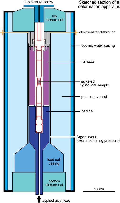
37

Provided the temperatures are sufficient, rocks begin to creep at low stresses. It means that ductile
parts of the lithosphere are very weak in comparison to the elastic-rigid lithospheric parts and may be
treated as viscous at long time scales.

 Brittle-ductile transition
The effect of increased confining pressure is to inhibit fracturing and cracking. As the confining
pressure (i.e. the lithostatic pressure in the Earth) is increased the behaviour of rocks passes through
a transition from brittle to ductile behaviour for each particular type of rock. This brittle-ductile
transition is generally placed at the lower limit of most crustal seismicity. This transition is not sharp,
nor is it a consistent depth or temperature. It is a function of hydrostatic pressure, temperature and
strain rate as well. In general, the lower the temperature and hydrostatic pressure, and the higher the
strain rate, the more likely is a rock to behave in a brittle manner. Conversely, the higher the
temperature and hydrostatic pressure and the lower the strain rate (or the longer time the stress is
applied), the more likely is a rock to behave in a ductile manner. In reality, there is a broad transition
between brittle and ductile behaviours, where “semi-brittle” or “semi-ductile” deformation involves
a mixture of frictional sliding and ductile flow on the microscale.

STRESS AND STRAIN IN ROCKS
Rocks and minerals are natural solid materials. To investigate the behaviour of rocks and relate strain
and strain rates with stress, one need to experimentally deform rocks under varied and controlled
conditions of temperature, pressure, fluids and time. Such experiments are the foundation of rock
mechanics.

 Most mechanical tests consist in compressing a small cylindrical rock sample along its axis with a
piston while exerting a confining pressure to all sides of the sample with a pressurised fluid. The fluid,
contained in a pressure chamber, transmits a uniform confining pressure to the rock cylinder through
an impermeable, flexible sleeve called jacket, made of a material (usually copper) sufficiently weak
at experimental conditions to not distort measurements. The confining pressure simulates the pressure
to which rocks deep in the Earth are subjected, i.e. the weight of the overlying rock. The axial
compression replicates a geologically realistic tectonic force. This experimental setting is known as
triaxial test because it allows predetermining stress to be applied along each of the three principal
axes, with the main compression oriented parallel to the cylinder long axis. However, two of the
principal stresses are equal to the confining pressure.
The stress along the axis of the cylinder is calculated knowing the axial force applied by the piston
and the area of the cylinder extremities. The difference between the axial stress and the confining
pressure is the differential stress (σ1 − σ 3 ) . Pore pressure, if necessary, is introduced through
additional devices. By varying any or all the pressures (axial load, confining and pore pressures), one
can obtain different stress configurations: The axial stress can be either larger (compression) or
smaller (tensile) than the confining pressure. Axial loading allows only few % of strains. Experiments
reaching high shear strains are in torsion, whereby samples are twisted between coaxially rotating
plates.

jpb – Strength profiles Tectonics, 2019

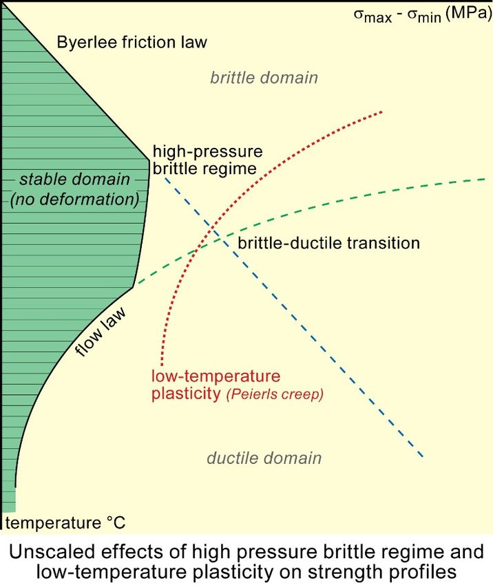
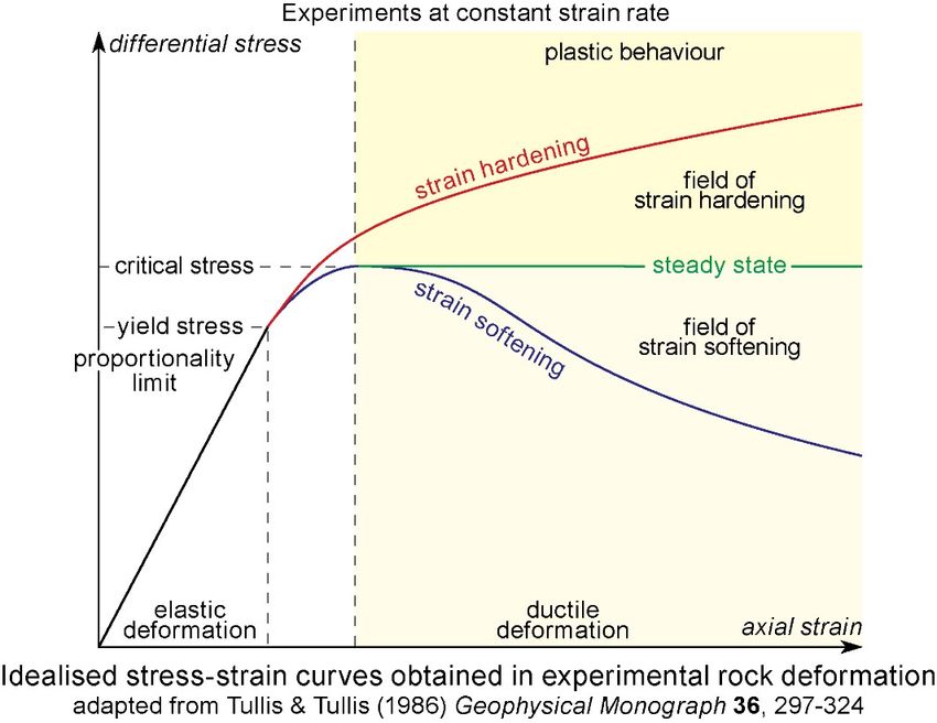
38

Results are graphically displayed in diagrams where the differential stress (σ1 − σ 3 ) is plotted against
the strain ε , which is calculated from the measured displacement of the piston ∆ reported to the
initial length of the specimen  0 : ε =∆  0 . This displacement is timed to access strain rate. The
detailed shape of the stress/strain curve depends on the rate of loading, and on other parameters that
will be discussed after a general description.

Constant strain-rate experiments - Effects of variation in stress
In constant strain rate experiments, the piston of the machine moves at a constant rate throughout the
experiment. The specimen deforms at a constant rate. In order to maintain this rate, the stress is
allowed to vary and this is recorded. Three main fields in terms of progressive increase in tension
(elastic, viscous and final break = ultimate failure) can be identified on a typical strain-time diagram.

jpb – Strength profiles Tectonics, 2019

39

 Elasticity limit
Starting from the origin, i.e. at the onset of experiment, the stress-strain graph begins with a straight
linear segment along which the strain increment is proportional to the stress increment. The sample
recovers its initial size as soon as the load is removed.

This linear plot documents that the rock first deforms as a perfectly elastic material. The stress
corresponding to the end of this linear section is called proportionality limit. For slightly larger
values of differential stress, a change in slope of the stress-strain graph indicates the beginning of
permanent deformation: The stress is no longer proportional to strain. The point where permanent
strain begins is the yield point (corresponding to a yield stress). This critical stress is generally
difficult to identify accurately because the stress-strain graph starts to curve rather gradually. In most
jpb – Strength profiles Tectonics, 2019

40
materials the proportionality and the yield points are practically the same. For other materials, such as
rubber, the segment of the stress-strain graph between the proportionality limit and the higher yield
point documents inelasticity (i.e. non-linear elasticity).

 Strain hardening
Continuing an experiment at low temperatures, the slope of the stress-strain graph of many materials
diminishes but remains positive beyond the yield point. An ever-increasing (but slower than in the
elastic domain) stress is required for deformation to increase from the yield point onward. The material
exhibits essentially ductile behaviour while undergoing irrecoverable deformation. This effect is the
strain hardening.
Strain hardening reflects intracrystalline deformation. Deformation displaces atoms of the crystal
lattice with the introduction of dislocations, which in turn create local elastic strain. The movement of
these dislocations (dislocation glide) results in permanent deformation. The dislocation density
increases, hence the elastic energy in the crystal lattice increases during hardening, which explains
why the material becomes stronger. Inversely, strain hardening can be suppressed by prolonged but
moderate heating (recovery) or by intense heating that induces a total recrystallization of the material
(annealing).
 Resilience
Strain hardening is responsible for another phenomenon. If load is removed during an experiment,
the unloading stress-strain curve is linear and has the same slope as its initial, elastic part, down to the
strain axis. Elastic strain is recovered but strain due to ductile-plastic deformation remains. Unloading
does not interrupt the stress-strain curve. If a load is reapplied to the same sample, it follows the same
line as the unloading path up to the point where unloading was prompted. Reinitiated deformation is
again elastic, but the new elasticity limit is higher than the first one (note that the slope, the elasticity
modulus, remains the same, though). Then the strain hardening curve resumes.
The yield strength of the specimen has increased (work hardening) because the original fabric, thus
properties of the sample, has been modified by permanent plastic deformation. The rock has acquired
more resilience.

Resilience is the strain energy stored per unit volume of material before failure. Elastic materials give
back the strain energy they absorbed when load is removed before failure.

jpb – Strength profiles Tectonics, 2019

41
 Stress relaxation
If the experiment is interrupted and the specimen held at constant strain, the stress will relax slowly.
If loading is resumed, the specimen will behave as if it had been unloaded and reloaded elastically up
to the point where straining was interrupted. Stress relaxation does not interrupt the stress-strain curve.

 Steady state
The yield strength is a variable that depends on the past plastic deformation of the sample. At high
temperatures or slow strain rates, the curve becomes horizontal from the yield point onward: no strain
hardening accompanies permanent deformation, and conditions approach steady state. Strain
increases indefinitely with no increase in stress. This slow deformation, known as creep, is the
essential characteristic of plastic strain. A perfectly plastic material is in steady state at the yield stress,
and from that point on the stress-strain graph.
Steady state follows minor strain softening in most rocks.

 Strain softening
Above a second critical value of highest stress known as the ultimate strength, the stress-strain curve
may descend either to a plateau value or (ultimately and) to a failure point. The material needs
progressively lower stresses to further deform. This behaviour is called strain softening.

 Failure
The stress-strain curve falls to finish the experimental strain softening or steady state. The material
exhibits accelerated viscous flow (necking for tension experiments) leading to rupture at the failure
stress. Breakage of the sample occurring before the yield point is brittle failure.

Shear fracture criteria
At rupture, the normal stress σ N and the shear stress σS acting on a plane are related by an equation
of the form:
 σS = f ( σ N ) (6)

jpb – Strength profiles Tectonics, 2019

42
and experiments have shown that, for materials with no cohesion strength such as soils, the
relationship is
 σS = σ N tan φ
where φ is known as the angle of internal friction (it is in this linear equation the slope of a line).
The term internal friction describes a material property of slip resistance along the fracture.

 Coulomb criterion
Coulomb proposed in 1773 that shear fracture occurs when the shear stress on a potential fault plane
reaches and overcomes a critical value. The relationship (6) becomes the Coulomb failure criterion:
 σS = c + µ σ N (7)
where c is a material constant known as the cohesion or the shear strength;
 µ is another material constant known as the coefficient of internal friction equivalent to the
term tan φ seen for soils.

Equation (7) assumes that shear fracture in solids involves two factors: breaking cohesive bonds
between particles of intact rock (the c term), together with frictional sliding (the term µ , proportional
to the normal compressive stress σ N acting across the potential fracture plane). This physical
interpretation predicts a linear increase of rock strength with normal stresses acting on the rock and
fits reasonably well much experimental data. Experiments provide cohesive strength of the order of
10-20 MPa for most sedimentary rocks and 50 MPa for crystalline rocks. The average angle of internal
friction is 30°.
The Coulomb criterion predicts that shear fractures form at less than 45° to σ1 because of the positive
slope of the shearing resistance curve and the symmetrical shape of the shear stress curve. This
criterion, also termed Mohr-Coulomb and Navier-Coulomb yield criterion, governs the creation of a
new fracture.

 Byerlee’s law
The frictional strength on fault planes is generally constant. The coefficient of internal friction µ on
existing fractures in consolidated rocks determines which shear stress is required to cause further
movement on the fault planes:
 σS = µ σ N (8)
This equation, usually valid when two rough surfaces are in contact, is known as Amonton’s law. A
direct consequence of this law (and the Coulomb criterion) is that the shear stress required for sliding
is independent of the surface contact area and increases with normal stress, therefore with confining
pressure. The parameter µ , in this general sense, is also referred to as the coefficient of static friction.
James Byerlee, an American geophysicist, compiled experimentally determined values of the shear
stress required for frictional sliding on pre-cut fault surfaces in a wide range of rock types. He found
two best-fit lines that depend on the confining pressure. For confining pressures corresponding to
shallow crustal depths (up to 200 MPa ≈ 8 km ), µ = 0.85 and equation (8) becomes:
 σS= 0.85 σ N (9)
Two diagrams actually illustrate this linear function.
The first one refers to very low (

43

The second one fits laboratory results generated under higher (up to 100 MPa) normal stress
conditions.

jpb – Strength profiles Tectonics, 2019

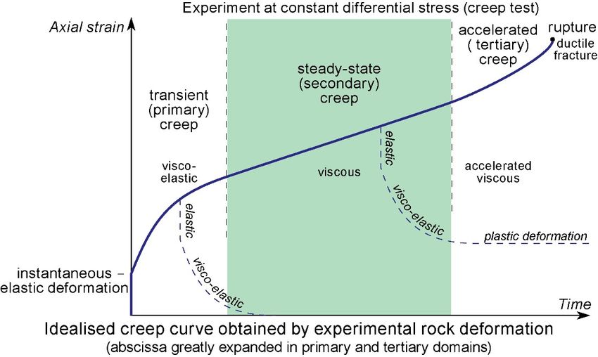
44
The large scatter of data point under very low normal stress reflects surface roughness, the area of
contact of the asperities, less influent under higher confining pressure because the latter prevents
dilatancy of the shear fracture, hence unlocking of interwoven surface irregularities. Instead, shearing
and smearing of asperities tends to stabilize frictional properties
For confining pressures between 200 and 2000 MPa, the frictional strength of pre-cut rocks is better
described by including a "cohesion-like" parameter:
 =σS 50MPa + 0.6 σ N (10)

The Byerlee’s law refers to equations (9) and (10), together. They are empirical and indicate that the
shear stress required to activate frictional slip along a pre-existing fracture surface is largely
insensitive to the composition of the rock. These laws seem to be valid for normal stresses up to 1500
MPa and temperatures < 400°C, which allows defining a lower boundary to stresses acting in the
brittle lithosphere.

Constant stress experiments - Ductile flow
Deformation experiments lasting for days at constant differential stress and temperature produce very
slow, continuous and plastic creep (time-dependent flow) of the sample. The resulting strain / time

jpb – Strength profiles Tectonics, 2019

45
curve can generally be divided, after the initial elastic response, into three regions representing
decelerating, steady (constant rate) and accelerating creep:
In the first region, the slope of the curve (i.e. the strain rate) decreases progressively; this decelerating
behaviour is called primary or transient creep; it is logarithmic because the total strain increases
with the logarithm of time. The phenomenon of decreasing creep rate at constant stress is called cold
working, a strain hardening because the material becomes less ductile with increasing strain. Primary
creep is reversible if experimental load is ended, visco-elastic strain being slowly removed after
instantaneous retrieval of the elastic strain. Primary creep strain is usually < 1% of the sum of the
three creep regions.

- In the second, usually largest regions of creep curves, the slope (strain rate) is constant and
residual, plastic strain is irrecoverable; this linear flow behaviour is called secondary or steady-state
creep. Even with a constant stress steady-state creep could continue indefinitely. It may represent the
long-term deformation processes that occur within the Earth over geological times without failure.
Therefore it is the part of the experiment that interests most geologists. The material behaves like a
viscous, yet non-Newtonian fluid. As a first order but approximate explanation, steady-state creep
results from recovery processes (mostly thermal softening) balancing strain hardening (due to
dislocations) as it appears.
- In the third region, not always observed or absorbing a very small amount of strain, the strain
rate increases exponentially until rupture of the specimen. Accelerating flow is mainly caused by
the spread of microfractures or slip surfaces through the rock in such a way that they link up
(accumulating damage) to form continuous pervasive cracks causing loss of cohesion, and failure;
this is called tertiary or accelerating creep.

 Failure criteria
Ductile isotropic materials have equal or nearly equal strength values in uniaxial tension and uniaxial
compression. Yield is generally caused by the slip of crystal planes along the plane of maximum shear
stress. Therefore, and independent from the state of stress, a given point in the an isotropic body does
not deform plastically as long as the maximum shear stress at that point is under the yield shear stress,
which defines plasticity.
 Tresca criterion
The maximum shear stress criterion, known as Tresca criterion, assumes that the differential stress
and the maximal principal stress are smaller than the plastic, yield shear strength K:

jpb – Strength profiles Tectonics, 2019

46
 In uniaxial compression: σ1 ≤ K
 In uniaxial tension: σ3 ≤ K
 In general: ( σ1 − σ3 ) ≤ K
Graphically, this criterion requires that the two principal stresses plot within an irregular hexagon of
a two-dimensional space.

The six-sided prism in the two-dimensional stress space is an hexagon of infinite length in the along
the hydrostatic axis, inclined at 45° to all principal stress axes (planes of maximum resolved shear
stress are at 45° to stress axes).
 Von Mises criterion
The maximum distortion energy (a.k. von Mises) criterion, states that ductile failure occurs when the
energy of distortion per unit volume of isotropic material reaches the same energy for yield/failure.
Mathematically, this is expressed as
 1
 
 
 ( σ1 − σ2 )2 + ( σ2 − σ3 )2 + ( σ3 − σ1 )2  ≤ K 2
 2
The left side of this equation is known as equivalent stress, and the equation holds regardless the
relative magnitudes of σ1 , σ2 and σ3 . In plane stress, σ2 = 0 and the criterion reduces to:
 σ12 − σ1σ3 + σ32 ≤ K 2
This equation represents a principal stress ellipse in which the Tresca hexagon is inscribed. This
geometrical relationship shows that the maximum shear stress criterion is more conservative than the
von Mises criterion since it lies inside the von Mises ellipse. Like for the Tresca criterion, the ellipse
has infinite length in the σ1 =σ2 =σ3 , i.e. the hydrostatic axis direction (the ellipse actually is an
oblique section of an infinite cylinder).

jpb – Strength profiles Tectonics, 2019

47

Deformation tests yield results better reproduced by the von Mises stress than by the Tresca criterion.

 Steady-state creep function
Creep mechanisms depend strongly on temperature. Dislocation glide is dominant in the lower
temperature range, giving way to dislocation and lattice diffusion (Nabarro-Herring) creep at
increasing temperature, followed by grain boundary diffusional (Coble) creep at very high
temperature. These mechanisms are not described here. In general, the differential stress (σ1 −σ 3 ) is
related to the rate of steady state creep ε by the non-linear, empirical (phenomenological) equation
of the form:
 −Q + pV
 ε = Aσn d − m f fluid
 r
 exp
 RT
where A, the frequency factor, is a material constant defined for the particular creep mechanism in
 − ∙ −1.
 σ the differential stress
 n is also an experimentally determined constant depending on the material and the creep
 mechanism; it commonly varies between 3 and 5, but can be higher for dislocation glide.
 d is the grain size with exponent −m
 f fluid is the fluid fugacity (generally water) with exponent r
 Q is a creep activation energy, a constant that must be determined experimentally. Q has a
 unit of kcal (or Joules) / mole.
 p is pressure
 V the activation volume
 R is the gas constant (in ∙ −1 ∙ −1 ).
 T is the absolute temperature in Kelvin
Grain size and fluid fugacity have nearly no effect on dislocation creep because it results from
practically rigid displacement of matter by motion of within crystal lattice defects (the dislocations).
The generalized equation is thus reduced to:
 dε n −Q
 ε
 = = A ( σ1 − σ3 ) exp (11)
 dt RT
The right part of equation (11), referred to as Weertman equation, implies that viscosity decreases
exponentially with temperature. High temperature diffusion creep involves the additional grain size,
power law dependency and A includes a diffusion coefficient. Since diffusion implies material
jpb – Strength profiles Tectonics, 2019