MAGNIFICENT BEASTS OF THE MILKY WAY: HUNTING DOWN STARS WITH UNUSUAL INFRARED PROPERTIES USING SUPERVISED MACHINE LEARNING - DIVA PORTAL
←
→
Page content transcription
If your browser does not render page correctly, please read the page content below
.

Magnificent beasts of the Milky Way: Hunting
 down stars with unusual infrared properties
     using supervised machine learning

                              Julia Ahlvind1
                        Supervisor: Erik Zackrisson1
                       Subject reader: Eric Stempels1
                          Examiner: Andreas Korn1
              Degree project E in Physics – Astronomy, 30 ECTS
       1
           Department of Physics and Astronomy – Uppsala University
                               June 22, 2021
Contents
1 Background 2
1.1 Introduction . . . . . . . . . . . . . . . . . . . . . . . . . . . . . . . . . . . . . . . . . . . . . . . . 2
2 Theory: Machine Learning 2
2.1 Supervised machine learning . . . . . . . . . . . . . . . . . . . . . . . . . . . . . . . . . . . . . . . 3
2.2 Classification . . . . . . . . . . . . . . . . . . . . . . . . . . . . . . . . . . . . . . . . . . . . . . . 3
2.3 Various models . . . . . . . . . . . . . . . . . . . . . . . . . . . . . . . . . . . . . . . . . . . . . . 3
2.3.1 k-nearest neighbour (kNN) . . . . . . . . . . . . . . . . . . . . . . . . . . . . . . . . . . . 3
2.3.2 Decision tree . . . . . . . . . . . . . . . . . . . . . . . . . . . . . . . . . . . . . . . . . . . 4
2.3.3 Support Vector Machine (SVM) . . . . . . . . . . . . . . . . . . . . . . . . . . . . . . . . 4
2.3.4 Discriminant analysis . . . . . . . . . . . . . . . . . . . . . . . . . . . . . . . . . . . . . . 5
2.3.5 Ensemble . . . . . . . . . . . . . . . . . . . . . . . . . . . . . . . . . . . . . . . . . . . . . 6
2.4 Hyperparameter tuning . . . . . . . . . . . . . . . . . . . . . . . . . . . . . . . . . . . . . . . . . 6
2.5 Evaluation . . . . . . . . . . . . . . . . . . . . . . . . . . . . . . . . . . . . . . . . . . . . . . . . . 6
2.5.1 Confusion matrix . . . . . . . . . . . . . . . . . . . . . . . . . . . . . . . . . . . . . . . . . 6
2.5.2 Precision and classification accuracy . . . . . . . . . . . . . . . . . . . . . . . . . . . . . . 7
3 Theory: Astronomy 7
3.1 Dyson spheres . . . . . . . . . . . . . . . . . . . . . . . . . . . . . . . . . . . . . . . . . . . . . . . 8
3.2 Dust-enshrouded stars . . . . . . . . . . . . . . . . . . . . . . . . . . . . . . . . . . . . . . . . . . 8
3.3 Gray Dust . . . . . . . . . . . . . . . . . . . . . . . . . . . . . . . . . . . . . . . . . . . . . . . . . 9
3.4 M-dwarf . . . . . . . . . . . . . . . . . . . . . . . . . . . . . . . . . . . . . . . . . . . . . . . . . . 10
3.5 post-AGB stars . . . . . . . . . . . . . . . . . . . . . . . . . . . . . . . . . . . . . . . . . . . . . . 10
4 Data and program 10
4.1 Gaia . . . . . . . . . . . . . . . . . . . . . . . . . . . . . . . . . . . . . . . . . . . . . . . . . . . . 11
4.2 AllWISE . . . . . . . . . . . . . . . . . . . . . . . . . . . . . . . . . . . . . . . . . . . . . . . . . 11
4.3 2MASS . . . . . . . . . . . . . . . . . . . . . . . . . . . . . . . . . . . . . . . . . . . . . . . . . . 11
4.4 MATLAB . . . . . . . . . . . . . . . . . . . . . . . . . . . . . . . . . . . . . . . . . . . . . . . . . 12
4.4.1 Decision trees . . . . . . . . . . . . . . . . . . . . . . . . . . . . . . . . . . . . . . . . . . . 12
4.4.2 Discriminant analysis . . . . . . . . . . . . . . . . . . . . . . . . . . . . . . . . . . . . . . 13
4.4.3 Support Vector Machine . . . . . . . . . . . . . . . . . . . . . . . . . . . . . . . . . . . . . 13
4.4.4 k-nearest neighbour . . . . . . . . . . . . . . . . . . . . . . . . . . . . . . . . . . . . . . . 13
4.4.5 Ensemble . . . . . . . . . . . . . . . . . . . . . . . . . . . . . . . . . . . . . . . . . . . . . 13
5 The general method 14
5.1 Forming datasets and building DS models . . . . . . . . . . . . . . . . . . . . . . . . . . . . . . . 14
5.1.1 Training set stars . . . . . . . . . . . . . . . . . . . . . . . . . . . . . . . . . . . . . . . . . 14
5.1.2 Training set Dyson spheres . . . . . . . . . . . . . . . . . . . . . . . . . . . . . . . . . . . 14
5.1.3 Training set YSOs . . . . . . . . . . . . . . . . . . . . . . . . . . . . . . . . . . . . . . . . 16
5.2 Finding and identifying the DS candidates . . . . . . . . . . . . . . . . . . . . . . . . . . . . . . . 16
5.2.1 Manual analysis of DS candidates . . . . . . . . . . . . . . . . . . . . . . . . . . . . . . . 16
5.3 Testing set . . . . . . . . . . . . . . . . . . . . . . . . . . . . . . . . . . . . . . . . . . . . . . . . 17
5.4 Best fitted model . . . . . . . . . . . . . . . . . . . . . . . . . . . . . . . . . . . . . . . . . . . . . 18
6 Process 18
6.1 limiting DS magnitudes . . . . . . . . . . . . . . . . . . . . . . . . . . . . . . . . . . . . . . . . . 19
6.2 Introducing a third class . . . . . . . . . . . . . . . . . . . . . . . . . . . . . . . . . . . . . . . . . 19
6.3 Coordinate dependence . . . . . . . . . . . . . . . . . . . . . . . . . . . . . . . . . . . . . . . . . 20
6.4 Malmquist bias . . . . . . . . . . . . . . . . . . . . . . . . . . . . . . . . . . . . . . . . . . . . . . 21
6.5 cc flag . . . . . . . . . . . . . . . . . . . . . . . . . . . . . . . . . . . . . . . . . . . . . . . . . . . 22
6.6 Feature selection . . . . . . . . . . . . . . . . . . . . . . . . . . . . . . . . . . . . . . . . . . . . . 22
6.7 Proportions of the training sets . . . . . . . . . . . . . . . . . . . . . . . . . . . . . . . . . . . . . 23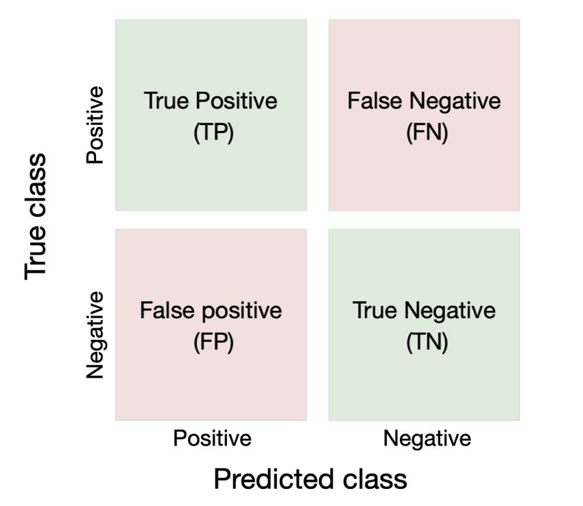
7 Result                                                                                                                                                                                            23
  7.1 Frequent sources of reference . . .               .   .   .   .   .   .   .   .   .   .   .   .   .   .   .   .   .   .   .   .   .   .   .   .   .   .   .   .   .   .   .   .   .   .   .   24
      7.1.1 Marton et al. (2016) . . . .                .   .   .   .   .   .   .   .   .   .   .   .   .   .   .   .   .   .   .   .   .   .   .   .   .   .   .   .   .   .   .   .   .   .   .   24
      7.1.2 Marton et al. (2019) . . . .                .   .   .   .   .   .   .   .   .   .   .   .   .   .   .   .   .   .   .   .   .   .   .   .   .   .   .   .   .   .   .   .   .   .   .   24
      7.1.3 Stassun et al. (2018) . . . .               .   .   .   .   .   .   .   .   .   .   .   .   .   .   .   .   .   .   .   .   .   .   .   .   .   .   .   .   .   .   .   .   .   .   .   24
      7.1.4 Stassun et al. (2019) . . . .               .   .   .   .   .   .   .   .   .   .   .   .   .   .   .   .   .   .   .   .   .   .   .   .   .   .   .   .   .   .   .   .   .   .   .   25
  7.2 A selection of intriguing targets . .             .   .   .   .   .   .   .   .   .   .   .   .   .   .   .   .   .   .   .   .   .   .   .   .   .   .   .   .   .   .   .   .   .   .   .   25
      7.2.1 J18212449-2536350 (Nr.1) .                  .   .   .   .   .   .   .   .   .   .   .   .   .   .   .   .   .   .   .   .   .   .   .   .   .   .   .   .   .   .   .   .   .   .   .   26
      7.2.2 J04243606+1310150 (Nr.8)                    .   .   .   .   .   .   .   .   .   .   .   .   .   .   .   .   .   .   .   .   .   .   .   .   .   .   .   .   .   .   .   .   .   .   .   27
      7.2.3 J18242978-2946492 (Nr.10)                   .   .   .   .   .   .   .   .   .   .   .   .   .   .   .   .   .   .   .   .   .   .   .   .   .   .   .   .   .   .   .   .   .   .   .   28
      7.2.4 J18170389+6433549 (Nr.22)                   .   .   .   .   .   .   .   .   .   .   .   .   .   .   .   .   .   .   .   .   .   .   .   .   .   .   .   .   .   .   .   .   .   .   .   29
      7.2.5 J14492607-6515421 (Nr.26)                   .   .   .   .   .   .   .   .   .   .   .   .   .   .   .   .   .   .   .   .   .   .   .   .   .   .   .   .   .   .   .   .   .   .   .   30
      7.2.6 J06110354-4711294 (Nr.30)                   .   .   .   .   .   .   .   .   .   .   .   .   .   .   .   .   .   .   .   .   .   .   .   .   .   .   .   .   .   .   .   .   .   .   .   31
      7.2.7 J05261975-0623574 (Nr.37)                   .   .   .   .   .   .   .   .   .   .   .   .   .   .   .   .   .   .   .   .   .   .   .   .   .   .   .   .   .   .   .   .   .   .   .   32
      7.2.8 J21173917+6855097 (Nr.46)                   .   .   .   .   .   .   .   .   .   .   .   .   .   .   .   .   .   .   .   .   .   .   .   .   .   .   .   .   .   .   .   .   .   .   .   33
  7.3 Summary of the results . . . . . .                .   .   .   .   .   .   .   .   .   .   .   .   .   .   .   .   .   .   .   .   .   .   .   .   .   .   .   .   .   .   .   .   .   .   .   34

8 Discussion                                                                                                                                                                                        34
  8.1 Evaluation of the approach . . . . . . . .                        .   .   .   .   .   .   .   .   .   .   .   .   .   .   .   .   .   .   .   .   .   .   .   .   .   .   .   .   .   .   .   35
      8.1.1 The influence of various algorithms                         .   .   .   .   .   .   .   .   .   .   .   .   .   .   .   .   .   .   .   .   .   .   .   .   .   .   .   .   .   .   .   35
      8.1.2 Training sets . . . . . . . . . . . .                       .   .   .   .   .   .   .   .   .   .   .   .   .   .   .   .   .   .   .   .   .   .   .   .   .   .   .   .   .   .   .   36
  8.2 Challenges . . . . . . . . . . . . . . . . . .                    .   .   .   .   .   .   .   .   .   .   .   .   .   .   .   .   .   .   .   .   .   .   .   .   .   .   .   .   .   .   .   37
  8.3 Follow-up observations . . . . . . . . . . .                      .   .   .   .   .   .   .   .   .   .   .   .   .   .   .   .   .   .   .   .   .   .   .   .   .   .   .   .   .   .   .   37
  8.4 Grid search . . . . . . . . . . . . . . . . .                     .   .   .   .   .   .   .   .   .   .   .   .   .   .   .   .   .   .   .   .   .   .   .   .   .   .   .   .   .   .   .   38
  8.5 Future prospects and improvements . . .                           .   .   .   .   .   .   .   .   .   .   .   .   .   .   .   .   .   .   .   .   .   .   .   .   .   .   .   .   .   .   .   39

9 Conclusion                                                                                                                                                                                        40

A Appendix                                                                                                                                                                                          i
  A.1 Candidates . . . . . . . .    .   .   .   .   .   .   .   .   .   .   .   .   .   .   .   .   .   .   .   .   .   .   .   .   .   .   .   .   .   .   .   .   .   .   .   .   .   .   .   .   i
  A.2 Uncertainty derivations .     .   .   .   .   .   .   .   .   .   .   .   .   .   .   .   .   .   .   .   .   .   .   .   .   .   .   .   .   .   .   .   .   .   .   .   .   .   .   .   . iii
  A.3 Results of various models     .   .   .   .   .   .   .   .   .   .   .   .   .   .   .   .   .   .   .   .   .   .   .   .   .   .   .   .   .   .   .   .   .   .   .   .   .   .   .   . iv
  A.4 Algorithm . . . . . . . . .   .   .   .   .   .   .   .   .   .   .   .   .   .   .   .   .   .   .   .   .   .   .   .   .   .   .   .   .   .   .   .   .   .   .   .   .   .   .   .   . v
      A.4.1 linear SVM . . . .      .   .   .   .   .   .   .   .   .   .   .   .   .   .   .   .   .   .   .   .   .   .   .   .   .   .   .   .   .   .   .   .   .   .   .   .   .   .   .   . v
      A.4.2 quadratic SVM . .       .   .   .   .   .   .   .   .   .   .   .   .   .   .   .   .   .   .   .   .   .   .   .   .   .   .   .   .   .   .   .   .   .   .   .   .   .   .   .   . vii
Abstract The significant increase of astronomical data necessitates new strategies and developments to analyse a large amount of information, which no longer is efficient if done by hand. Supervised machine learning is an example of one such modern strategy. In this work, we apply the classification technique on Gaia+2MASS+WISE data to explore the usage of supervised machine learning on large astronomical archives. The idea is to create an algorithm that recognises entries with unusual infrared properties which could be interesting for follow-up observations. The programming is executed in MATLAB and the training of the algorithms in the classification learner application of MATLAB. Each catalogue; Gaia+2MASS+WISE contains „ 109 , 5ˆ108 and 7ˆ108 (The European Space Agency 2019, Skrutskie et al. 2006, R. M. Cutri IPAC/Caltech) entries respectively. The algorithms searches through a sample from these archives consisting of 765266 entries, corresponding to objects within a ă 500 pc range. The project resulted in a list of 57 entries with unusual infrared properties, out of which 8 targets showed none of the four common features that provide a natural physical explanation to the unconventional energy distribution. After more comprehensive studies of the aforementioned targets, we deem it necessary for further studies and observations on 2 out of the 8 targets (Nr.1 and Nr.8 in table 3) to establish their true nature. The results demonstrate the applicability of machine learning in astronomy as well as suggesting a sample of intriguing targets for further studies.
Sammanfattning
     Inom astronomi samlas stora mängder data in kontinuerligt och dess tillväxt ökar snabbt för varje
år. Detta medför att manuella analyser av datan blir mindre och mindre lönsama och kräver istället
nya strategier och metoder där stora datamängder snabbare kan analyseras. Ett exempel på en sådan
strategi är vägledd maskininlärning. I detta arbete utnyttjar vi en vägled maskininlärnings teknik
kallad klassificering. Vi använder klassificerings tekniken på data från de tre stora astronomiska
katalogerna Gaia+2MASS+WISE för att undersöka användningen av denna teknik på just stora
astronomiska arkiv. Idén är att skapa en algorithm som identifierar objekt med okontroversiella
infraröda egenskaper som kan vara intressanta för vidare observationer och analyser. Dessa ovanliga
objekt är förväntade att ha en lägre emission i det optiska våglängdsområdet och en högre emission
i det infraröda än vad vanligtvis är observerad för en stjärna. Programmeringen sker i MATLAB och
träningsprocessen av algoritmerna i MATLABs applikation classification learner. Algoritmerna söker
igenom en samling data bestående av 765266 objekt, från katalogerna Gaia+2MASS+WISE. Dessa
kataloger innehåller totalt „ 109 , 5ˆ108 och 7ˆ108 (The European Space Agency 2019, Skrutskie
et al. 2006, R. M. Cutri IPAC/Caltech) objekt vardera. Det begränsade dataset som algoritmerna
söker igenom motsvarar objekt inom en radie av ă 500 pc. Många av de objekt som algoritmerna
identifierade som ”ovanliga” tycks i själva verket vara nebulösa objekt. Den naturliga förklaringen för
dess infraröda överskott är det omslutande stoft som ger upphov till värmestrålning i det infraröda.
För att eliminera denna typ av objekt och fokusera sökningen på mer okonventionella objekt gjordes
modifieringar av programmen. En av de huvudsakliga ändringarna var att introducera en tredje klass
bestående av stjärnor inneslutna av stoft som vi kallar ”YSO”-klassen. Ytterligare en ändring som
medförde förbättrade resultat var att introducera koordninaterna i träningen samt vid den slutgiltiga
klassificeringen och på så vis, identifiering av intressanta kandidater. Dessa justeringar resulterade i
en minskad andelen nebulösa objekt i klassen av ”ovanliga” objekt som algoritmerna identifierade.
Projektet resulterade i en lista av 57 objekt med ovanliga infraröda egenskaper. 8 av dessa objekt
påvisade ingen av det fyra vanligt förekommande egenskaperna som kan ge en naturlig förklaring
på dess överflöd av infraröd strålning. Dessa egenskaper är; nebulös omgivning eller påvisad stoft,
variabilitet, Hα emission eller maser strålning. Efter vidare undersökning av de 8 tidigare nämnda
objekt anser vi att 2 av dessa behöver vidare observationer och analys för att kunna fastslå dess sanna
natur (Nr.1 och Nr.8 i tabell 3). Den infraröda strålningen är alltså inte enkelt förklarad för dessa 2
objekt. Resultaten av intressanta objekt samt övriga resultat från maskininlärningen, visar på att
klassificeringstekniken inom maskininlärning är användbart på stora astronomiska datamängder.
List of Acronyms
Machine learning
ML – Machine learning.
model – Another word for the machine learning system or algorithm that is trained on the training data.
training data - A dataset that consists of both input and output data, which is used in the training process
of the models.
predictions- The output of a model after it has been trained on training data.
input data - The data that is fed to the model, i.e. the first part of the training data.
labeled data - Another word for the output data, i.e. the second part of the training data.
test data - A dataset that is used to test the performance of the model and that is different from the training
set.
training a model - A process where the algorithms are provided training data, where it learns to recognise
patterns.
hyperparameter - A parameter whose value is used to control the learning process, thus, adjusting the model
in more detail.
classifier - A method on solving classification problems.
kNN – k-Nearest Neighbour
SVM – Support Vector Machine
classes/labels - The output of a classifier.
parametric – For parametric models, the training data is used to initially establish parameters. However once
the model has been trained, the training data can be discarded, since it is not explicitly used when making
predictions.
loss function - A function that measures how well the model’s predicted output fits the input data.
TP – True positive.
FN – False negative.
FP – False positive.
TN – True negative.
Astronomy
SED – Spectral Energy Distribution.
YSO – Young Stellar Object.
PMS – Pre-main-sequence
MS – Main sequence
IR – Infrared
FIR – Far infrared
NIR – Near infrared
UV - Ultraviolet
DS – Dyson sphere
11 Background on large astronomical data. The procedure is to create
a sample of models of typical targets that contain
1.1 Introduction these unusual infrared properties, as well as a sample
of common stars. The unconventional objects, as the
Progress in astronomy has been driven by a number ones that fit the Dyson sphere models, are limited to
of important revolutions, such as the telescope, near solar-magnitudes within this study. Thereafter,
photography, spectroscopy, electronics and computers, we apply ML to train algorithm(s) to recognise and
which have resulted in a major burst of data. categorise stars with uncommon infrared properties
Astronomers are now facing new challenges of handling from the Gaia+WISE+2MASS catalogues. The Gaia
large quantities of astronomic data which accumulates archive is a grand ESA (European Space Agency)
every day. Large astronomical catalogues such as catalogue comprising brightnesses measurements and
Gaia, with its library of „1.6 billion stars, hold positions of more than 1.6 billion stars with remarkable
key information on stellar evolution, galaxy formation accuracy. The brightness is measured in the three
processes, the distribution of stars and much more. It passbands GBP (BP), G and GRP (RP) which covers
is crucial for the progression of astronomic research, wavelengths from the optical („300 nm) to near-
not only to access this data but to extract relevant infrared (NIR) („1.1 µm). The 2MASS (Two Micron
and important information. It is unrealistic to assume All Sky Survey) catalogue contains, besides astrometric
that all data will be manually analysed. Therefore, we data, ground-based photometric measurements in
are entering an era where we put more confidence in the NIR regime („1.1-2.4 µm), with around 470
computers and machine learning (ML) processes, to do million sources. Complementary to the optical-NIR
the work at hand. measurements, WISE (Wide-field Infrared Survey
The astronomic data avalanche is not solely the Explorer) photometry data is recovered in four mid-
cause of the increasing usage of ML. The technique infrared (mid-IR) bandpasses („2.5-28 µm). The
is becoming more and more popular and important in AllWISE source catalogue contains „ 7 ˆ 108 entries
numerous fields. Moreover, the growing interest is not (R. M. Cutri IPAC/Caltech). Note that this catalogue
isolated to astronomical research, but in other scientific is not a point source catalogue, meaning that it
research, financial computations, medical assistance contains some resolved sources such as galaxies and
and applications in our mobile phones. There are many filaments in galactic nebulosity. Using these three
subdivisions for machine learning that can be used archives enables a broader wavelength range, necessary
in various fields. For the purposes of this work, we for our study. The project is expected to result in a
will adopt supervised machine learning (SML). This list of intriguing objects that are suitable for follow-up
ML technique exploits the fact that the input data is observations. Questions that will be considered are; are
classified so that the predictions of the training can be there any objects with properties consistent with those
evaluated. This is in contrast to unsupervised machine expected for Dyson spheres in our night sky? If so, is
learning which trains models based on unclassified it possible to determine their nature based on existing
training data. Simply put, the difference between data outside the Gaia+WISE+2MASS catalogue?
unsupervised and supervised ML is, thus, that the
training process is further supervised for the latter In this report we include relevant background
technique. theory of machine learning and astronomical
Supervised ML can be further divided into knowledge in section 2 & 3, respectively. In section
subgroups, namely regression and classification 4, we review the databases used in the ML part of
techniques. The technicalities of the latter are the work, the programs and applications exploited in
discussed in section 2.2 and is used within this work. section 4.4 and the employed programming methods
The classifier method will be adapted in order to and scripts in section 5. Further on, in section 6, we
categorise stars with and without unusual infrared discuss the process and steps of implementations taken
properties. Several types of stars are expected to have throughout the work to improve the programs. The
these kinds of properties. Some of them being stars main results are thereafter appraised in section 7, as
surrounded by debris disks and dust-enshrouded stars, well as a selection of the most prosperous candidates.
such as young stellar objects (YSOs) or protostars. Thereafter we discuss the overall progress, results, the
Further intriguing objects with such infrared properties application of ML in astronomy and future prospects
are the hypothetical Dyson spheres (DS). A Dyson and improvements in section 8. Finally, we conclude
sphere is an artificial mega-structure which encloses the results of this work and its appliance in section 9.
a star with the porpoise of harvest the stellar light.
By narrowing down the search to the latter group of
alluring objects, we hope to discover intriguing targets 2 Theory: Machine Learning
that are not directly explained by previously observed
astronomical phenomena. Machine learning is the scientific area involving the
study of a computer algorithm that learns and
With this work, we aim to exploit the use of improves on past experiences. A ML algorithm or
machine learning and thereby test its applicability model is constructed on sample data, referred to as
2training data, with the goal to predict and asses 2. Therefore, the classes of the outcome can be referred
an outcome without being trained for that specific to as positive and negative classes.
task. There are two main subgroups of ML which
are used in various situations, unsupervised learning
and supervised learning. In the former technique,
the algorithm is trained to identify intrinsic patterns
2.3 Various models
within the input-training data without any knowledge There are many different models or algorithms that
of labeled responses (output data). A commonly used can be used in machine learning. Similar to the
technique of unsupervised ML is clustering. It is used choice of supervised or unsupervised machine learning,
to find hidden patterns and groupings in the data, different models are suitable for different purposes.
which has not been categorised or labelled. Instead Furthermore, the classification model that depends on
of relying on labeled data, the algorithm looks for the chosen machine learning algorithms, can further be
commonalities in the training data and categorises tuned by changing the values of the hyperparameters
entries according to presence or absence of these (see section 2.4). Some of the models commonly used
properties. The latter subgroup, supervised ML, is for classification, as described in the former section, are
used within this work and presented in the following discussed below. Note however, that these methods are
section. also applicable for other machine learning techniques
besides classification. The algorithms reviewed in the
2.1 Supervised machine learning following section are also the ones adapted in this work.
By trial and error we adopt the various algorithms
Supervised machine learning techniques utilise the to identify what algorithm(s) are most suited for this
whole training data which contains some input data, classification problem.
output data and the relationship between the two
groups. By using a model, that has previously been
adapted to the training data, one can predict the 2.3.1 k-nearest neighbour (kNN)
outcome i.e. the output data from a new set of data, The k-nearest neighbour method for supervised
that is different from the training data (Lindholm machine learning is, as many other SML models, based
et al. 2020). The process of adapting the model onto on the predictions of its neighbours. If an input
the training data is referred to as training the model. data point xi is close to a training data point xt ,
Unsupervised machine learning is particularly useful then the prediction of the input data yi (xi ) should
for cases where the relationship between the input data be close to the prediction of the training set yt (xt ).
x and output data y is not explicit. For instance, the For example, if k “ 1, then the object is assigned
relationship may be too complicated or even unknown the class of its single nearest neighbour. For higher
from the training data. Thus, the problem can not be values of k, the data point is classified by assigning
solved with a traditional computer program of input the label that is most prevailing among its k number
x that returns the output y, based on some common of nearest neighbours. The kNN algorithm works in
set of rules. Supervised machine learning, instead, various metric spaces. A common metric space is the
approaches the problem by learning the relationship Euclidean metric, where the distance between two data
between x and y from training data. points (xj , xi ) in n-dimensions follow eq. 1 (Kataria &
Singh 2013). Other examples of metric space that can
As previously mentioned, which ML approach to be used are Chebyshev or Minkowski.
use depends on the data and what you want to achieve.
SML is suitable for regression techniques, categorising g
or classifying data since the algorithm needs training fn
fÿ 2
in order to make predictions on the unseen data. Dpxj , xi q “ ||xj ´ xi || “ e pxi,k ´ xj,k q (1)
Regression techniques predict continuous responses e.g. k
changes in the flux of a star. In contrast, classification
techniques predict discrete responses e.g. what type As with all ML models, the parametric choices vary
of star it is. The latter approach will be used in this between problems. There is no optimal value for k
work and is more thoroughly described in the following which is profitable for the majority of cases and few
section. guidelines exist. However, one is that for a binary
(two-class) classification, it is beneficial to set k equal
to an odd number since this avoids tied classifications
2.2 Classification
(Hall et al. 2008). But in truth, one has to, by trial
The classification method categorises the output into and error, test the options on a training set to see
classes and can thus take M number of finite values. what is suitable for this particular classification. In
In the most simplest case, M=2 and is referred to general, a large value of k reduces the effect of noise
as a binary classification, if M ą2 we instead call it on the classification, but at the same time makes the
a multi-class classification. For the binary case, the boundaries between classes less distinct, thus risking
labelled responses are noted -1 and 1, instead of 1 and overfitting (the model has adapted too much to the
3training data and will not be able to generalise well to
new data).
2.3.2 Decision tree
Another method commonly used in machine learning is
decision trees and more specifically classification trees
if the problem regards classification. The leaves in
a classification tree represent the class labels and the
branches the combined features which are used in order
to select the class. More specifically, the input variable
(previously referred to as xi ) is known as the root node,
the last nodes on the tree are known as leaf nodes or
terminal nodes and the intermediate nodes are called
internal nodes.
The nodes of a decision tree are chosen by looking Figure 1: An illustration of a two dimensional support vector
machine with corresponding notations.
for the optimum split of the features. One function that
measures the quality of a split is the Gini index. This
function selects the optimal separation for when the
data is split into groups, where one class dominates and problem can be split into multiple binary classification
minimises the impurity of the two children nodes–the problems and thus be solved for. The primary
following nodes after a split of a parent node. The objective of this technique is to project nonlinear
gini impurity thus measures the frequency at which any separable n-dimensional data samples onto a higher
element of the dataset is miscategorised when labelled, dimensional space with the use of various kernel
and follows the formula seen in eq. 2. Here πˆlm is functions such that they can be separable by an n-
the proportion of the training observations in the lth dimensional hyperplane. This is referred to as a linear
region that belong to the mth class according to eq. 3. classifier but higher orders such as quadratic, cubic and
In eq. 3, nl is the number of training data points in Gaussian also exists. The choice of the hyperplane in
node l, yi is the ith label of the training data point the dimensional space is important for the precision
(xi , yi ). Therefore, πˆlm is essentially the probability and accuracy of the model.
of an element yi belonging to the class m (Lindholm One common choice is the maximum-margin
et al. 2020). hyperplane, where the distance between the two closest
data points of each group (the support vectors), is
M
ÿ M
ÿ maximised and that no miss classification occurs. The
Ql “ πˆlm p1 ´ πˆlm q “ 1 ´ pπˆlm q2 (2) hyperplane or the threshold which separates these two
m“1 m“1 classes will thus reside in between the two closest
points where the distance from the threshold and data
1 ÿ point is called the margin (Hastie et al. 2009). In two
πˆlm “ 1yi “ m (3)
nl dimensions, one can visualise the data as two groups
on the xy-plane, where one can draw two parallel lines
representing the boundary of each group, orthogonal
Trees can be sensitive to small changes in the to the shortest distance between the data points of
training data, which can result in large changes in the the different groups (see figure 1). For this case,
tree, hence in the final outcome of the classification. the hyperplane is also represented as a straight line
Therefore, the numbers of splits in classification trees and positioned in between the two boundary lines. A
must be treated carefully in order to prevent overfitting general hyperplane can be written as a set of points
i.e. where the tree does not generalise well from the x satisfying the eq. 4, where θ is the normal vector to
training data. In the use of decision trees, one can the hyperplane ( and y the classification label following
further improve the precision of the predicament by y P t ´1, `1 . The boundary lines (hyperplanes for
utilising the so-called pruning. Pruning is essentially a higher dimension) thus represent the position where
the inverse process of splitting an internal node when anything on or above eq. 5a is of the class with label 1,
a sub-node or internal node is removed after training and on or below eq. 5c of class -1. The distance between
the data. these two boundary hyperplanes in the θ-direction is
2
||θ|| (see figure 1), and to maximise the distance, ||θ||
2.3.3 Support Vector Machine (SVM) needs to be minimised (Lindholm et al. 2020).
Support vector machine is yet a further ML technique
well suited for classification, but can also be used in
regression problems. In its most simple form, SVM
does not support multiclass classification, however, the θT x ´ b “ y (4)
4constraints are followed. In other words, if C is large,
the constraints are hard to ignore and the margin is
θT x ´ b “ 1 (5a) narrow. If C is small, the constraints are easily ignored
θT x ´ b “ 0 (5b) and the margin is broad.
θ T x ´ b “ ´1 (5c)
ÿ
min||θ||2 ` C maxp0, 1 ´ yi pθ T xi ` bqq (8)
i
Furthermore, if we also require that all
classifications are correct, in addition to having the Furthermore, for non-linear separable data, even
maximum distance as stated above, we enforce eq. 7. introducing soft margins would not suffice. The
` ˘ kernel function provides a solution to this problem by
y θT xi ` b ě 1@i (7) projecting the data from a low-dimensional space to
a higher dimensional space (Noble 2006). The kernel
When combining the two criteria, we get the so- function derives the relationships between every pair
called optimisation` problem,˘where ||θi || is subject to of data points as if they are in a higher dimension,
the constraints yi θ T xi ´ b ě 1@1 . Thus, we end meaning that the function does not actually do the
up with the function signpθ T x ´ bq. The choice of transformation. This is referred to as the kernel trick.
the maximum margins is often by default used by the Common kernel functions are polynomials of degree
program itself since it is the most stable solution under two or three, as well as radial basis function kernels
perturbations of input of further data points. However, such as Gaussian.
for non linearly separable data, the algorithm often
finds the soft margins. This lets the SVM algorithm 2.3.4 Discriminant analysis
deal with errors in the data by allowing a few outliers
to fall on the wrong side of the hyperplane, thus Discriminant analysis uses the training set to
”misclassify” them without affecting the final result. determine the position of boundaries that separates
In other words, the outlier(s) instead reside on the the response classes. The locations of the boundaries
same side of the hyperplane with members of the are determined by treating each individual class as
opposite class. Clearly, we can not allow too many samples from multidimensional Gaussian distributions.
misclassifications, and thus aiming to minimise the The boundaries are thereafter drawn at the points
misclassification rate. Hence when introducing the where the probability of classifying an element to
soft margins it is necessary to control and check the either of the classes, is equal. The boundary is thus
process. Soft margins are used in a technique called a function that depends on the parameters of the
cross validation. This technique is used to control the fitted distributions. If the distribution of all classes
balance between misclassifications and overfitting. One is assumed to be equal, the boundary equations are
can set the number of allowed misclassifications within simplified greatly and become linear. Otherwise, the
the soft margins to get the best classification that is boundaries are quadratic. The quadratic discriminant
not overfitting. This happens automatically for some analysis (QDA) is slightly more demanding in terms
programs (like MATLABs classification learner (CL)) or of memory and calculations, but it is still seen as an
can be set manually. efficient classification technique. The QDA can be
In order to control the position of the boundary, expressed as seen in eq. 9 (Lindholm et al. 2020).
SVM utilises a so-called cost function. The idea is
to regulate the freedom of misclassified points on the ´ ¯
action of maximising the margin by using the hinge loss π̂m N x|µ̂m , Σ̂m
function. A point belonging to the positive class that ppy “ m|xq “ ř ´ ¯ (9)
M
resides on or above the higher boundary or support j“1 π̂j x|µ̂j , Σ̂j
vector (eq. 5a) has zero loss. A point of the positive
n
class on the threshold (eq. 5c) has loss one, and further Where π̂m{j “ m{j
n is the number of training points
points in the positive class on the ”wrong” side of in class m/j over the total number of data points and
the threshold have linearly increasing loss. The cost N indicates Gaussian or normal distribution. Eq. 10
function thus accounts for the distance between the shows the mean vector of each class among all training
support vector and the misclassified point. The further data points within that class.
the separation, the more costly it gets to correctly
classify the point and less so to shift the threshold, 1 ÿ
µ̂m{j “ xi (10)
maximise the margin and miscategorise the point. The nm{j i:yi “m
total cost function can be stated as seen in eq. 8 where
the first term governs the maximisation of the margin Finally, eq. 11 describes the covariance matrix of
and the second term accounts for the loss function each class m, in other words, a matrix that describes
(Smola & Schölkopf 1998). The parameter C is a the covariance between each pair of elements of the
regularisation parameter that adjusts how well the given vectors xi and µ̂m .
52.4 Hyperparameter tuning
Sometimes the performance of the classification
1 ÿ T
σ̂m “ pxi ´ µ̂m q pxi ´ µ̂m q (11) can be optimised by setting the hyperparameters
nm i:yi “m manually. Hyperparameters vary between models but
are generally seen as ”settings” for the algorithm.
A typical hyperparameter for SVM algorithms is the
polynomial degree of the kernel function, for kNN it
2.3.5 Ensemble is the number of neighbours k. For decision trees
there are two important hyperparameters to consider;
Ensemble methods are meta-algorithms that uses the number of estimators (decision trees) and the
several copies of a fundamental model. This set of maximum allowed depth for each tree, i.e. the
multiple copies are referred to as an ensemble of base maximum number of splits or branches. As with many
models, where base models can e.g. be one of the things in machine learning, there is no optimal choice
aforementioned models in the sections above. The of hyperparameters. Therefore, empirical trials of the
fundamental concept is to train each such base model hyperparameters are the preferred way to optimise the
in slightly different ways. Each base model makes its algorithm, this is also known as hyperparameter tuning.
own prediction and thereafter an average or majority Another approach is the so-called Grid search, which
vote is derived to obtain the final prediction (Lindholm builds and evaluates a model for each combination
et al. 2020). There are two main types of models of parameters specified in a grid. A third option
when discussing ensemble classification, bagging and is a random search which is based on a statistical
boosting. In bagging, or ”bootstrap aggregation”, distribution of each parameter, from which values are
multiple slightly different versions of the training set randomly sampled (Bergstra & Bengio 2012). This
are created. These sets are random overlapping subsets work is, as previously mentioned, executed in MATLAB
of the training data. This results in an ensemble of and MATLAB’s classification learner. Here the evaluation
similar base models which are not identical to the of the hyperparameter tuning is automatically done
core base model, thus when training the models, one by the program and commonly not tweaked by us.
reduces the variance and so the risk of overfitting. One However, hyperparameter tuning is indeed accessible
could summarise bagging as an ensemble of multiple in MATLAB and tested within this work. The available
models of the same type, where each one is trained and relevant hyperparameters in MATLABs CL is further
on a different generated random subset of the training discussed in section 4.4. Furthermore, we evaluate our
data. This method is not a new model technique, but experimentation of hyperparameter tuning by studying
a collection of formerly mentioned models that uses a a confusion matrix which is addressed in the below
new approach to the data itself. After the ensemble has section 2.5.1.
been trained, the results are aggregated by an average
or weighted average of the predicted class probabilities,
which results in a final prediction from the bagging. 2.5 Evaluation
The second ensemble classification technique 2.5.1 Confusion matrix
mentioned is boosting. In contrast to bagging, the
base models in boosting are trained sequentially where The most convenient way of evaluating the
each model aims to correct for the mistakes that the performance of a classifier is to study a so-called
former models have made. Furthermore, an effect confusion matrix. For a binary classification problem,
of using boosting is bias reduction of the base model, the confusion matrix is formed by separation of the
instead of the reduced variance in bagging. This allows validation data in four groups depending on the true
boosting to turn an ensemble of weak base models into output or label y and the predicted output ypxq.
one stronger model, without the heavy calculations Figure 2 shows a general confusion matrix where the
that normally would be required (Lindholm et al. green boxes, true positive (TP) and true negative
2020). Both boosting and bagging are ensemble (TN), show the correctly classified elements, meaning
methods that combine prediction from multiple models that the model predicts the true class. The red boxes,
of classification (or regression) type. Thus, boosting is false positive (FP) and false negative (FN) instead
also using previously mentioned models through a new show the number of incorrectly predicted elements.
approach. The biggest difference is, as mentioned, that Out of the latter two outcomes, the false positive is
boosting is sequential. The idea is that each model tries often the most critical one to consider and should,
to correct for the mistakes made by the previous one therefore, be minimised. This is true because, in most
by modifying the training dataset after each iteration, cases of classification, we are interested in discerning
in order to highlight the data points for which the one specific class as accurate as possible. To illustrate
formerly trained models performed dissatisfactory. this, we will use an example related to this work,
The final prediction is then a weighted average or namely the classification of common stars (A) and
weighted majority vote of all models of the ensemble. stars with unusual infrared properties (B). Since the
goal is to identify targets belonging to class B, TP are
6The accuracy of a classification model is similar to
the precision, but includes the total correct predictions
while precision evaluates half of the true outcome.
The accuracy thus evaluates the fraction of correct
predictions over the total number of predictions, as
seen in eq. 13. The ratio takes a value between 0
and 1, but the accuracy is commonly presented in
percentage 0-100%. The accuracy metric is conceivably
better suited for a uniformly distributed sample since
it is a biased representation of the minority class.
This implies that the majority class has a bigger
impact on the accuracy than what the minority class
has. Therefore, the classification accuracy could be
misleading if the working involves large differences in
the quantities of each class (Schütze et al. 2008).
TP ` TN
Figure 2: The figure shows a confusion matrix with true and Accuracy “ (13)
predicted classes. The true positive (TP) and true negative (TN) TP ` TN ` FP ` FN
(green squares) represents the correctly classified objects while
the false positive (FP) and the false negative (FN) (red squares) Naturally, a precision close to 1 and an accuracy
are the falsely classified objects.
near 100% is preferred, however, as discussed earlier
(section 2.5.1) it is more important to reduce the
targets predicted as, and truly are unusual stars. TN number of FN. A model with high precision and a
are targets predicted as and are common stars, FN are high ratio of FN is a worse model than one with lower
targets predicted as stars but belong to class A. Finally, precision and a low ratio of FN. Nevertheless, both
the most critical outcome, FP are targets predicted as parameters give a quick indication of how well the
group B but in reality, TN are targets predicted as and model classifies the entries.
are common stars, FN are targets predicted as stars but
belong to class A. Finally, the most critical outcome,
FP are targets predicted as group B but in reality, 3 Theory: Astronomy
belong to group A (common stars falsely classified as
unusual stars). If the number of FP is high, it means The purpose of this work is as previously mentioned,
that the model will assort many common stars as to utilise machine learning to select intriguing stellar
unusual ones, thus making the result unreliable. This targets with unusual infrared properties. A typical
means that the group of interest will be contaminated spectral energy distribution (SED) of a star, like a
by ”common stars” and, thereby making the manual black-body spectrum, is characterised by a relatively
process of checking the list of interesting targets time- smooth peak at some specific wavelength (e.g. see
consuming. If instead FN is high while FP is low, the SED of the Sun in figure 3). The placement of
it means that many uncommon targets are lost in the peak is determined by the temperature of the star
the classification and gets assorted into the common and indicates in what wavelength range the majority
group. It is true that these targets will go unnoticed, of the stellar radiation is emitted. The black-body
however, the targets later classified as uncommon stars curve of solar-like stars (spectral type FGK) commonly
by the model will have a smaller uncertainty of being peaks in the optical wavelength range and decreases
misclassified. as we move to longer wavelengths in the infrared
(IR). The specific position of the peak in the optical
signifies the colour of the star. It should be noted that
2.5.2 Precision and classification accuracy black-body radiation is often the first approximation
Further parameters that can be used for assessing the for stellar emission even though stars are not perfect
overall performance of the classification is precision black bodies. The unconventional objects considered in
and classification accuracy. The precision of a model this study are expected to deviate from this classical
describes the ratio of true positives over all positives, view. The targets of interest do indeed show a peak
as stated in eq. 12. A high precision value (close to in the optical, but with a lower brightness than a
1) is good and a low (close to 0) signals that there is common star. Furthermore, these targets are also
a problem in the classification which yields many false expected to show an excess in the infrared regime.
positives. The underlying idea is that there is some component
blocking a significant fraction of the stellar radiation,
TP thus making the star dimmer. However, the stellar
precision “ (12) radiation can not be retained within but is re-emitted
TP ` FP
in another wavelength. This re-emitted radiation is the
7are identifying potential candidates based on their IR-
excess from thermal radiation. The AGENT formalism
is one proposal of how the energy budget would look
like for a Dyson sphere. This formalism was first
introduced by Wright, Griffith, Sigurdsson, Povich &
Mullan (2014) and follows;
α`“γ`ν (14)
ff Where α is the collected starlight, is the non-
starlight energy supply, γ represent the waste heat
radiation and ν is all other forms of energy emission
e.g. neutrino radiation. For simplifications of the
formalism one assumes negligible non-thermal losses
(ν „ 0) and that the energy from starlight is much
higher than other sources ( „ 0) thus generalising
Figure 3: The solar spectrum. Credit: Robert A. eq. 14 to α “ γ. The simplified black body model of
Rohde licensed under CC BY-SA 3.0 the Dyson sphere can be expressed using α and γ on
the host star (see eq. 6 of Wright, Griffith, Sigurdsson,
Povich & Mullan (2014)). We generalise it further by
thermal radiation emitted in the IR. In the following expressing the luminosity and magnitude of the DS as;
section, we will discuss known astronomical objects
that fit the description of these uncommon targets, as LDS “ LStar ˆ fcov (15)
well as a hypothetical object which lay the ground for
our investigation of the use of ML on large astronomical
datasets. magDS “ magStar ´ 2.5log10 p1 ´ fcov q (16)
3.1 Dyson spheres 3.2 Dust-enshrouded stars
Perhaps the most speculative candidate for a target One type of the known astronomical objects that
with a SED as described in the above section is a so- fit part of the SED profile of our DS models are
called Dyson sphere. A Dyson sphere is an artificial dust-enshrouded stars or certain stars within nebulae.
circumstellar structure first introduced by Dyson Young stellar objects (YSOs) are good candidates
(1960), which harvest starlight from the enclosed star. for nebulous objects. YSOs denotes stars in their
Such a mega-structure covers parts of or the whole early stage of evolution and can be divided into two
star, thus blocking the star’s light. This causes the subgroups; protostars and pre-main-sequence (PMS)
energy output in the optical part of the SED to stars. The terminology of a protostar refers to a
drop. However, the blocked starlight is reradiated point in time of the cloud collapsing phase of stellar
in the thermal infrared as the megastructure gets formation. When the density at the centre of the
heated up and has turned into an ember the size collapsing cloud has reached around 10´10 kgm´3 , the
of a star. This energy output is seen as a second region becomes optically thick and makes the process
peak or slope in the IR range of the SED. Stars more adiabatic (no heat or mass transferred between
encased by Dyson spheres are therefore expected to system and surrounding). The pressure increases in the
show abnormalities in their SED when compared to central regions and eventually reaches near hydrostatic
”normal” stars. A Dyson sphere is typically not equilibrium (the gravitational force is balanced by
visualised as a solid shell enclosing the star, but rather the pressure gradient; Carroll & Ostlie (2017)). The
a swarm of satellites where each satellite absorbs a protostar resides deep within the parent molecular
small fraction of the stellar radiation (Suffern 1977, cloud, enshrouded in a cocoon of dust. Since the
Wright, Mullan, Sigurdsson & Povich 2014, Zackrisson star has yet to begin nuclear fusion, the generated
et al. 2018). The covering fraction fcov , depends on the energy does not come from the core. Instead, most
distribution and scales of the enshrouding satellites. of the energy comes from gravitational contractions
If one assumes that this astro-engineered structure which heats the interior. The heated dust thereafter
acts like a gray-absorber (all wavelengths are equally reradiates the photons in longer wavelengths which
affected), one expects only a general dimming of the accounts for the IR source of radiation associated with
observed flux and no further changes on the spectral these stars. This IR excess might, therefore, resemble
shape. An ideal Dyson sphere with high efficiency that of a Dyson sphere. However, the protostar is not
can absorb all stellar light and has minimal energy expected to peak much in optical due to the dust which
loss. In reality, that is not likely the case for such is fully enshrouds the protostar, thus all radiation is
a construction. Some of the absorbed stellar light reprocessed.
will be turned into waste heat and other forms. The As the name suggests, a PMS star is a star in the
waste heat is the centrepiece of this work since we evolutionary stage just before the main sequence where
8Tauri stars, they also show strong emission lines. The
major difference between T Tauri and Herbing Ae/Be
stars are their masses, where the former typically have
masses in the range 0.5 to 2 M@ (solar masses) and
the latter group 2-10 M@ .
Furthermore, YSOs are associated with early
star evolution phenomena such as protoplanetary
disks (also known as proplyds), astronomical jets (a
beam of ionised matter that is emitted along the
axis of rotation) and masers. Maser emission is
commonly detected via emission from OH molecules
(hydroxyl radical) or water molecules H2 O. A maser
is the molecular analogue to a laser and a source of
stimulated spectral line emission. Stimulated emission
is a process where a photon of specific energy interacts
with an excited atomic electron which causes the
electron to drop into a lower energy level. The emitted
photon and the incident photon will be in the same
phase with each other, thus amplify the radiation
(Carroll & Ostlie 2017).
Figure 4: The HR diagram with absolute magnitude and
luminosity on the vertical axis and spectral class and effective
temperature on the horizontal axis. The diagram also shows the
different evolutionary stages of stars and some well known stars.
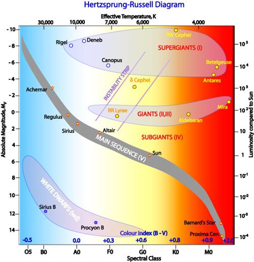
Image credit: R. Hollow, CSIRO. 3.3 Gray Dust
most stars in their evolution reside today and spend A potential source that could give rise to false high
most of their lifetime. The main sequence (MS) fcov Dyson sphere candidates, is seemingly grey dust.
refers to a specific part of the evolutionary track for Obscured starlight with no significant reddening of
a star in the so-called Hertzsprung-Russell diagram the spectrum is likely caused by material in the line
(HR diagram), which plots the temperature, colour of sight. This is what we refer to as grey dust.
or spectral type of stars against their luminosity or Micrometre-sized dust grains would essentially be grey
absolute magnitude, to mention a few versions (see at optical to near-infrared wavelengths, thus, reduce
figure 4). After a protostar has blown away its envelope the optical peak that is seen for most stars, similarly
or birth cradle, it is optically visible. The young star as expected of a Dyson sphere (Zackrisson et al. 2018).
has acquired nearly all of its mass at this stage but Studies suggest that such dust grains have been formed
has not yet started nuclear fusion. Thereafter, the star in circumstellar material around supernovae (Bak
contracts, which results in an internal temperature Nielsen et al. 2018) but have also been detected in the
increment and finally initiates fusion processes. When interstellar medium (Wang et al. 2015). Observations
the star is in the phase of contraction, it is in the have shown that the µm-sized graphite grains, together
pre-main-sequence stage (Larson 2003). Two common with nano- and submicron-sized silicate and graphite
types of PMS stars are T Tauri stars and Herbing grains, fit the observed interstellar extinction of the
Ae/Be stars. T Tauri stars are named after the first Galactic diffuse interstellar medium in the range from
star of their class to be discovered (in the constellation far-UV to mid-IR, along with NIR to millimetre
of Taurus) and represent the transition between stars thermal emission (Wang et al. 2015). The µm-sized
that are still shrouded in dust and on the MS. Dust grains account for the flat or grey extinction in the
that surrounds the young star (both T Tauri and UV, optical and NIR. Since they absorb little (near no)
Herbing Ae/Be type) is the source of IR radiation and amount in the optical, they do not emit much radiation
causes the IR excess in the SED which matches the DS in the IR. The sources of smaller sized grains could,
models. However, the T Tauri stars are expected to however, potentially mimic the IR signature of a DS.
feature irregular luminosity variations due to variable The gray dust likely affects the optical part of the SED
accretion and shocks, with timescales on the order more than the IR, to a great extent. Interstellar gray
of days (Carroll & Ostlie 2017). Furthermore, these dust will block the dispersed stellar radiation from a
types of young stars exhibit strong hydrogen emission distant star and emit IR radiation while gray dust that
lines (the Balmer series). Thus, an Hα spectral line surrounds a star prevents a larger fraction of the stellar
indication is a good signature for these types of stars. radiation to escape, hence also a higher IR emission.
Herbing Ae/Be stars are likely high-mass counterparts Therefore, the IR property created by circumstellar
to T Tauri stars. As the name suggests, these stars dust, is the one that most resembles that of a Dyson
are of spectral type A or B and in likeness to T sphere.
93.4 M-dwarf
M-dwarfs or Red dwarfs are small and cool main
sequence stars (thus appear red in colour) and
constitutes the largest proportion of stars in Milky
Way, more than 70% (Henry et al. 2006). These low-
mass stars develop slowly and can therefore maintain
a near-constant low luminosity for trillions of years.
This makes them both the oldest existing types of
stars observed, but also very hard to detect at large
distances. Evidently, not all M-dwarfs have debris
disks. In fact, this group of stars is rare and most
observed M-dwarfs with debris disks are younger M-
dwarfs, (Binks & Jeffries 2017). Most studies of
circumstellar debris disks are concentrated on early-
type or solar-type stars, and less so for M-dwarfs.
However, some studies (Avenhaus et al. 2012, Lee et al.
2020) have shown that warm circumstellar dust disks
are not only observed around M-dwarfs but that they
also create an excess in the IR. The underlying sources Figure 5: Evolutionary track of a solar mass star. Credit:
of the dust disks are believed to be planetesimal belts Lithopsian, licensed under CC BY-SA 4.0.
where the dust is created through collisions. This also
takes place in the solar system, however, the collisions
are more frequent for other observed systems which IR, thus producing similar SEDs as the ones expected
results in higher IR excess than solar system debris for DSs. However, the obscured AGB stars, and young
disks (Avenhaus et al. 2012). The combination of stars as previously discussed, are often associated with
the low luminosity, temperature and an encompassing OH masers. The post-AGB phases start when the
debris disk of an M-dwarf could create a SED that is star begins to contract and heat up. The increasing
consistent with a DS model. Although, a debris disk is temperature and constant luminosity make the star
not expected to generate high coverage, meaning that a transverse horizontally towards higher temperatures in
fitted DS model onto a target with a debris disk should the HR diagram (see figure 5). When the temperatures
show a low covering fraction. Typically a debris disk reach „ 25000 K, the radiation is energetic enough to
reduces the optical emission in orders of LLIR‹
„ 0.01 ionise the remaining circumstellar envelope and appear
(Hales et al. 2014). as planetary nebulae (Engels 2005). It is possible that
post-AGB or non-pulsating AGBs have similar SEDs
3.5 post-AGB stars as the expected DSs since both objects are assumedly
cooler with stronger IR-emission.
Post-Asymptotic giant branch (post-AGB) stars are
evolved stars with initial masses of 1-8 M@ (Engels
(2005), values vary significantly between authors „0.5-
10 M@ ). These objects are expected to have high 4 Data and program
brightness where a solar-mass star can reach ą 1000
times the present solar luminosity (see figure 5). An
AGB star is both very luminous and cool, thus having The data used within this work originates from three
strong IR-radiation and occupy the upper right region different catalogues. These are the Gaia (Data release
in the HR-diagram seen in figure 5. The characteristics 2, DR2; Gaia Collaboration (2016, 2018)), 2MASS
of these stars are the energy production in the double- (Skrutskie et al. 2006) and WISE/AllWISE (All Wide-
shell structure (helium and hydrogen) that surrounds field Infrared Survey Explorer; Wright et al. (2010)).
the degenerated carbon-oxygen core. The AGB phase The three catalogues cover different wavelength ranges,
can be divided into two parts; early-AGB, a quiescent that when used together covers optical to mid-infrared
burning phase and the thermal pulse phase, where wavelengths. Since the targets of interest display
large energy releases are created by flashes of He- somewhat lower energy output in the optical and an
shell burning. In these phases, the outer layers of excess in the IR, this range of wavelengths is suitable
the envelopes are extended to cooler regions by the for our project.
pulsation which facilitates dust formation. The newly
formed dust is pushed out by radiation pressure which In this section, we will first go through the
drags the gas along and leads to high mass-loss rates. three data catalogues from which we recover our
In turn, the high mass-loss rates lead to the formation astronomical data. Thereafter, a more in-depth review
of circumstellar dust shells with high optical depths. of machine learning via MATLAB, its features and
The dust absorbs the stellar light and re-emits in the utilities.
104.1 Gaia
The ESA space observatory Gaia with the
accompanying database is one of today’s greatest
resource of stellar data. The satellite is constantly
scanning the sky, thus creating a three-dimensional
map of no less than „ 1.6 billion stars. This
corresponds to around one per cent of the total number
of stars within the Milky Way. Furthermore, the
data will reach remarkable accuracy, where targets
brighter than 15m will have a position accuracy of
24 microarcseconds (mas) and the distance to the
nearest stars, as good as 0.001% (The European Space
Agency 2019). Such precision will be achieved at the
end of the mission when the satellite has measured
each target about 70 times. The satellite operates in Figure 6: The coloured lines show the passbands for GBP pBP q
three band-pass filters; BP , G and RP with respective (blue), G (green) and GRP pRP q (red) that defines the Gaia DR2
central wavelength; 0.532, 0.673 and 0.797 µm (Gaia photometric system. The thin, gray lines show the nominal, pre-
launched passbands used for DR1 and published in Jordi et al.
Collaboration 2016, 2018) which can be seen in figure 6. (2010). Credits: ESA/Gaia/DPAC, P Montegriffo, F. De Angeli,
New data releases are frequently published in the C. Cacciari. The figure was acquired from Gaia’s homepage
Gaia archive as the satellite repeatedly scans each where it was published 16/03/2018.
target. The latest release EDR3 was made public
in December of 2020. This work is based on the catalogue superior to a former WISE All-Sky
predecessor DR2. Even though the (early) EDR3 has Release Catalog. Furthermore, the photometric
better accuracy, it is missing some properties (such accuracy of AllWISE, in all four bands, has improved
as luminosity) and partly other properties for some due to corrections of the source flux bias and more
targets (e.g. G magnitudes). It is worth noting that the robust background estimations. The only exception,
errors of the magnitudes are not given in the archive, where WISE All-Sky is better than AllWISE is for
these are manually derived from the respective flux (see photometry measurements for sources brighter than
eqs. 30 & 31). The error estimation is a simplification the saturation limit in the first two bands W 1 ă 8 &
of the real uncertainty but is not expected to have an W 2 ă 7. Both these catalogues are commonly shown
impact on the machine learning process. The estimated for our Dyson sphere candidates when searched for in
errors for Gaia photometry in Vega system is based on VizieR 2 , where we pay extra attention to the variability
the derivation found on the homepage of ESA Gaia: flag for each band. From this catalogue we also utilise
GDR2 External calibration1 (Paolo Montegriffo 2020). a parameter called cc-flag which is discussed more in-
The derivation can be seen in Appendix A.2. depth in section 6.5.
4.3 2MASS
4.2 AllWISE
Between 1997 and 2001, the Two Micron All
WISE is a Medium Class Explorer mission by NASA Sky Survey resulted in photometric and astrometric
that conducted a digital imaging survey of the full measurements over the entire celestial sphere. A pair
sky in the mid-IR bandpasses; W 1, W 2, W 3 and of two identical telescopes at Mount Hopkins, Arizona
W 4 with respective central wavelength; 3.4, 4.6, 12.0 and Cerro Tololo, Chile, made NIR observations which
and 22.0 µm (Wright et al. 2010). The catalogue resulted in a Point Source Catalogue containing above
contains photometry and astrometry for over 500 470 million sources. The 2MASS All-Sky Data Release
million objects. In likeness to the Gaia satellite, the includes the aforementioned Point Source Catalogue,
WISE space telescope accumulates data for each target 4.1 million compressed FITS images of the entire sky
multiple times. The independent exposures for each and an additional Extended Source Catalogue of 1.6
point on the Ecliptic plane were typically 12 times million objects. The NIR photometric bands used
or more, while observational points at the Ecliptic in 2MASS and utilised within this work were; J, H
poles reached several hundred. In November 2013 the and Ks with corresponding central wavelengths; 1.247,
AllWISE Data Release was generated. This source 1.645 and 2.162 µm (Skrutskie et al. 2006). These
catalogue is a combination of data from WISE Full passbands largely correspond to the common bands J,
Cryogenic, 3-Band Cryo and NEOWISE Post-Cryo H and K, first introduced by Johnson (1962), with
survey phases. This has enhanced the sensitivity in the adjustment that 2MASS Ks filter (s for short)
the W 1 and W 2 bands, thus making the AllWISE excludes wavelengths beyond 2.31 µm to minimise
1 https://gea.esac.esa.int/archive/documentation/GDR2/Data_processing/chap_cu5pho/sec_cu5pho_calibr/ssec_cu5pho_
calibr_extern.html
2 https://vizier.u-strasbg.fr/viz-bin/VizieR
11You can also read