Master Thesis Evaluating pre-trained language models on partially unlabeled multilingual economic corpora
←
→
Page content transcription
If your browser does not render page correctly, please read the page content below

Master Thesis

Evaluating pre-trained language models on partially
     unlabeled multilingual economic corpora

                          Author
                        Jacopo Rizzo

                        Supervisors
    Prof. Dr. Christian Heumann, Dr. Matthias Aßenmacher
                         Advisors
        Prof. Dr. Ralf Elsas, M.Sc. Moritz Scherrmann

                  Department of Statistics
          Ludwig-Maximilians-Universität München
                 Munich, 26th of April 2022

Declaration of Authenticity

The work contained in this thesis is original and has not been previously submitted
for examination which has led to the award of a degree.

  To the best of my knowledge and belief, this thesis contains no material previously
published or written by another person except where due reference is made. This
applies also to all graphics, drawing, maps, tables and images included in this thesis.

            Place and Date                                 Jacopo Rizzo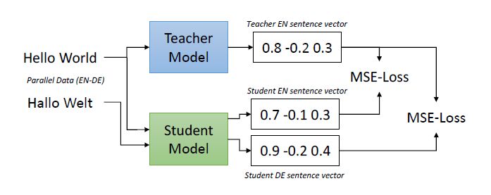
Abstract

   This master thesis analyses economic text documents of public companies and
aims to set up a transformer-based NLP model, which is able to automatically clas-
sify such documents in one or more self-defined classes. Specifically, the goal of this
thesis is to fine-tune a pre-trained BERT model on documents of German public
companies, and use this model to classify documents of American public companies.
Therefore, we evaluate the model on two different, but related, data sources, which
is comparable to evaluating a transfer learning problem. These documents can be
divided into three main categories: labeled German documents from German public
companies, unlabeled English documents from German companies and unlabeled
English documents from American companies. As we are primarily interested in
classifying the American documents, we make use of the labeled German data con-
taining the same content of the English documents of the German companies to
automatically label the latter, in order to have a labeled English dataset that can
be used for fine-tuning. The results show that our model partly outperforms the
chosen benchmark model by about 4 percentage points on the F1-score.
Contents

List of Figures                                                                          I

List of Tables                                                                          II

List of Abbreviations                                                                  III

1 Introduction                                                                          1

2 Problem Description and Related Works                                                 3
   2.1   Related works . . . . . . . . . . . . . . . . . . . . . . . . . . . . . . .    4

3 Methods                                                                               6
         3.0.1   Neural Networks in NLP . . . . . . . . . . . . . . . . . . . . .       8
   3.1   Word Embeddings . . . . . . . . . . . . . . . . . . . . . . . . . . . .        9
         3.1.1   Static Embeddings . . . . . . . . . . . . . . . . . . . . . . . . 10
         3.1.2   Tokenization . . . . . . . . . . . . . . . . . . . . . . . . . . . . 12
   3.2   Transformers . . . . . . . . . . . . . . . . . . . . . . . . . . . . . . . 14
         3.2.1   Attention! . . . . . . . . . . . . . . . . . . . . . . . . . . . . . 16
   3.3   BERT . . . . . . . . . . . . . . . . . . . . . . . . . . . . . . . . . . . 18
   3.4   Multilingual Transformers . . . . . . . . . . . . . . . . . . . . . . . . 20

4 Data                                                                                 24
   4.1   Original Data . . . . . . . . . . . . . . . . . . . . . . . . . . . . . . . 24
         4.1.1   Labels . . . . . . . . . . . . . . . . . . . . . . . . . . . . . . . 26
   4.2   Labels Transfer . . . . . . . . . . . . . . . . . . . . . . . . . . . . . . 28
   4.3   Transfer Evaluation . . . . . . . . . . . . . . . . . . . . . . . . . . . . 30
   4.4   Forms 8-K . . . . . . . . . . . . . . . . . . . . . . . . . . . . . . . . . 33

5 Fine-Tuning and Results                                                              35
   5.1   Fine-Tuning . . . . . . . . . . . . . . . . . . . . . . . . . . . . . . . . 36
   5.2   Test Data and Threshold Decision . . . . . . . . . . . . . . . . . . . . 38
   5.3   Transfer learning on forms 8-K . . . . . . . . . . . . . . . . . . . . . . 41
         5.3.1   TL on items 7 and 8 . . . . . . . . . . . . . . . . . . . . . . . 42
6 Discussion and Outlook 45 7 Conclusion 47 Bibliography 48 A Mathematics 53 A.1 CBOW and Skip-gram . . . . . . . . . . . . . . . . . . . . . . . . . . 53 A.2 Softmax function . . . . . . . . . . . . . . . . . . . . . . . . . . . . . 54 A.3 Word order in self-attention . . . . . . . . . . . . . . . . . . . . . . . 54 B Data Overview 56 B.1 Available features in each dataset . . . . . . . . . . . . . . . . . . . . 56 B.2 Labels’ definitions . . . . . . . . . . . . . . . . . . . . . . . . . . . . . 57 C Forms 8-k items 59 D Labels Transfer Evaluation 61
List of Figures

 3.1    NN representation . . .      .   .       .   .   .   .   .   .   .   .   .   .   .   .   .   .   .   .   .   .   .   .   .    7
 3.2    CBOW ans Skip-gram .         .   .       .   .   .   .   .   .   .   .   .   .   .   .   .   .   .   .   .   .   .   .   .   11
 3.3    WP tokenization . . . .      .   .       .   .   .   .   .   .   .   .   .   .   .   .   .   .   .   .   .   .   .   .   .   13
 3.4    Transformers . . . . . .     .   .       .   .   .   .   .   .   .   .   .   .   .   .   .   .   .   .   .   .   .   .   .   14
 3.5    Attention . . . . . . . .    .   .       .   .   .   .   .   .   .   .   .   .   .   .   .   .   .   .   .   .   .   .   .   16
 3.6    BERT architecture . . .      .   .       .   .   .   .   .   .   .   .   .   .   .   .   .   .   .   .   .   .   .   .   .   18
 3.7    BERT input embeddings        .   .       .   .   .   .   .   .   .   .   .   .   .   .   .   .   .   .   .   .   .   .   .   19
 3.8    BERT pre-training . . .      .   .       .   .   .   .   .   .   .   .   .   .   .   .   .   .   .   .   .   .   .   .   .   20
 3.9    SBERT . . . . . . . . .      .   .       .   .   .   .   .   .   .   .   .   .   .   .   .   .   .   .   .   .   .   .   .   21
 3.10   Knowledge distillation .     .   .       .   .   .   .   .   .   .   .   .   .   .   .   .   .   .   .   .   .   .   .   .   22

 4.1    Data relation . . . . . .    .   .       .   .   .   .   .   .   .   .   .   .   .   .   .   .   .   .   .   .   .   .   .   24
 4.2    Data overview . . . . . .    .   .       .   .   .   .   .   .   .   .   .   .   .   .   .   .   .   .   .   .   .   .   .   25
 4.3    Class distribution . . . .   .   .       .   .   .   .   .   .   .   .   .   .   .   .   .   .   .   .   .   .   .   .   .   27
 4.4    Multilingual embeddings      .   .       .   .   .   .   .   .   .   .   .   .   .   .   .   .   .   .   .   .   .   .   .   29
 4.5    Items distribution . . . .   .   .       .   .   .   .   .   .   .   .   .   .   .   .   .   .   .   .   .   .   .   .   .   33

 5.1    Accuracy dev set . . . . . . . . . . . . . . . . . . . . . . . . . . . 36
 5.2    BERT loss . . . . . . . . . . . . . . . . . . . . . . . . . . . . . . . 38
 5.3    Predictions items 7 and 8 . . . . . . . . . . . . . . . . . . . . . . 43

                                             I
List of Tables
4.1 Classes overview . . . . . . . . . . . . . . . . . . . . . . . . . . . 26
4.2 Allocation of classes and items . . . . . . . . . . . . . . . . . . . 28
4.3 Confusion matrix examples . . . . . . . . . . . . . . . . . . . . . 31
4.4 Confusion matrix for SBERT . . . . . . . . . . . . . . . . . . . . 32
5.1 Thresholds performances . . . . . . . . . . . . . . . . . . . . . . . 39
5.2 Local performance test set . . . . . . . . . . . . . . . . . . . . . . 40
5.3 GerBERT global performances . . . . . . . . . . . . . . . . . . . 40
5.4 Local performances 8-K . . . . . . . . . . . . . . . . . . . . . . . 41
5.5 Global performances 8-K . . . . . . . . . . . . . . . . . . . . . . . 42
5.6 Performances items 7 and 8 . . . . . . . . . . . . . . . . . . . . . 43
IIList of Abbreviations
AI Artificial Intelligence
BaFin Bundesanstalt für Finanzdienstleistungsaufsicht
BERT Bidirectional Encoder Representations from Transformers
BPE Byte Pair Encoding
CLS Classification Token
CNN Convolutional Neural Networks
DL Deep Learning
GRU Gated Recurrent Unit
LM Language Model
LSTM Long Short-term Memory
ML Machine Learning
MLM Masked Language Modelling
NLP Natural Language Processing
NN Neural Networks
NSP Next Sentence Prediction
RNN Recurrent Neural Networks
SBERT Sentence Bidirectional Encoder Represenations from Transformers
SEC U.S. Securities and Exchange Commission
SEP Separation Token
SGD Stochastic Gradient Descent
STS Semantic Textual Similarity
TL Transfer Learning
WP WordPiece
IIIChapter 1
Introduction
In economics, as in many other fields, it is essential to create the conditions to
ensure the fairness for all parties involved. This becomes particularly important
when dealing with listed companies, as it is not unusual for them to have a large
number of stakeholders, who must be informed simultaneously whenever the compa-
nies take important decisions. This transparency is fundamental for a fair market.
Thus, listed companies are obliged to publish specific documents reporting all the
relevant information about important corporate events or valuable disclosures every
time these occur (SEC, 2022). In Germany these kind of reports are best known
as Ad-Hocs and are regularised and controlled by the Bundesanstalt für Finanzdi-
enstleistungsaufsicht (BaFin), which is the German Federal Financial Supervisory
Authority, while in the United States these are named forms 8-K and the U.S. Se-
curities and Exchange Commission (SEC), the American counterpart of the BaFin,
clearly defines in which occasions these are required. These documents contain in-
formation that is considered material (Kenton, 2022), which means that there is a
high probability that investors will take them into great consideration when making
an investment decision. For example, a company publishes information concerning
internal changes in the Executive Board. Or a pharmaceutical company announces
the results of tests on a new drug that they plan to market. Normally a company
releases a variable amount of such documents during a year. Taking all listed compa-
nies into account, this results in a large amount of documents. It therefore becomes
very difficult for an investor to have a constant overview of various companies and
to filter the documents that may be relevant for him. Automating this process
would bring numerous advantages and of course would eliminate the likelihood of
human errors. The automation of processes like this is becoming more and more
important, especially when dealing with a big amount of data. In this regard, the
advent of Artificial Intelligence (AI) models has provided incredible improvements
in terms of results. And the branch of AI that deals with analysing and process-
ing text data, and more generally the natural language used by human beings, is
1better known as Natural Language Processing (NLP). In particular, in this field
research is carried out to teach machines to understand and analyse natural lan-
guage in different manners. And as with most modern AI models, artificial neural
networks often form the basis of many NLP models. Although the idea of this
type of model was already presented in the mid-1990s by Rosenblatt (1958), they
have gained notoriety and only found a significant and regular application in recent
decades. This is mainly due to the constantly increasing computational powers of
CPUs and GPUs in recent years, with which it is nowadays possible to train and use
AI models capable of tackling different NLP tasks with remarkable results, as for
example summarising newspaper articles, answering messages automatically, as in
the case of chat-bots, or classifying documents into defined categories. In this sense,
a significant increase in performance in this AI area was achieved with the introduc-
tion of the transformer-based models by Vaswani et al. (2017). Transformers have
partially revolutionised the world of NLP by succeeding in solving mathematical
and technical problems present in previous models. They also paved the way for
pre-trained models, i.e. models trained from scratch on a vast quantity of data that
can be generally used as a starting point for various challenges. And among the first
models with a transformer-based architecture, BERT is certainly one of the most
important, being capable of achieving outstanding results in several NLP tasks.
The goal of this thesis is to implement an NLP model, which is able to classify
economic documents in pre-defined classes. More precisely we want to fine-tune
a pre-trained BERT model using the Ad-Hocs, which we will then use to classify
the forms 8-K. Fine-tuning a model means taking the pre-trained version of it and
training it further on a specific task using the own data. The problem or task for
which we optimise the model with this process is also called the downstream task. In
our case this amounts to optimising the model to perform a multi-label classification.
This work is structured in the following way: In the next chapter we will introduce
the problem setting in detail and will provide some related works. In chapter 3
all the models and methods used in this work will be explained, with a particular
attention on transformers and BERT. Chapter 4 provides some descriptive statistics
and describes the pre-processing steps we have done on the data, while in chapter 5
we analyse and interpret the results of our classification model. These will be further
discussed in chapter 6, where we also present some ideas on what can be done to
improve our results. Chapter 7 will draw the final conclusions of this thesis. Note
that this work was done in cooperation with the Chair of Finance and Banking of
the LMU Munich, whom we will refer to as the project partner and who provided
us with the topic and the data.
2Chapter 2
Problem Description and Related
Works
In this thesis we want to set up a classification method that automatically classifies
economic documents, i.e. the forms 8-K, into pre-defined classes. We will use a total
of 22 classes, defined by the project partner, which we will look at more in detail in
chapter 4. Each document can be classified in, and thus belong to, more than a single
class. This means, that we face a so-called multi-label classification problem, i.e. a
single instance can be assigned to more classes1 . For example, a document reporting
the quarterly financial results and informing that a new CEO will replace the current
one would then belong to the classes Earnings and Management simultaneously.
Bit since the forms 8-K are not labeled with our classes, they cannot be used for
the fine-tuning process. Instead, labeled Ad-Hocs are available for the scope of this
thesis. We will make use of these to create a suitable dataset for fine-tuning a BERT
model. We are going to use the latter in turn to classify the forms 8-K. This process
of using a classification model trained on some specific data to classify other data,
which is related to some extent to the former one, can be seen as a kind of Transfer
Learning (TL) problem. As Bengio et al. (2003, p. 526) defines it, TL "refer to
the situation where what has been learned in one setting is exploited to improve
generalisation in another setting". With respect to this, the language of the labeled
Ad-Hocs represents the first major obstacle we have to deal with. The labeled Ad-
Hocs that we have are only in German language. Fine-tuning a BERT model in
one language and using it to classify text in another language would not be very
reasonable, because one, it was not optimised for a multilingual context and two,
most languages do not share much of their vocabularies, thus the shared knowledge
would be limited. Consequently, a BERT model trained on a single language is more
reliable than a model trained on more languages. Fortunately, many of the German
1
This is in contrast to a multi-class classification problem, where a single instance can belong
to only one class, i.e. the classes are mutually exclusive
32.1. RELATED WORKS
public companies, obligated to publish such documents, do so in both languages, i.e.
German and English, with both versions containing exactly the same information.
We are therefore confronted with a multilingual context, where we have partially
labeled data, i.e. the German Ad-Hocs, and partially unlabeled data, i.e. the English
Ad-Hocs. But we can make use of the fact that both language versions of a given
Ad-Hoc contain the same semantic information, to label the English one according
to the German one. This will set up a labeled English dataset, which can be used to
fine-tune BERT. With this we can then finally classify the forms 8-K in our classes.
A first classification for specific categories defined by the SEC is actually already
supplied with the forms 8-K. These categories are called items and the SEC defines
31 different ones. Each company filing such reports, needs to specify to which items
the single sections of the form belong to. The main reason, why we do not use these
already defined classes for our problem is that the definitions of these classes are
really vague and shallow. The two most frequent items for example, are defined
as Regulations and Other events and account alone for a third of the forms 8-K,
despite the fact that these contain information which belongs to other categories as
well. Hence, we want our model to be able to allocate categories to the disclosures
in a more fine-grained manner. While fine-tuning such a model seems feasible, a
second major problem arises when evaluating it. The inconsistency of the number
and definitions between our classes and the US items makes it difficult for us to
judge whether our model is able to correctly classify the single documents or not.
In order to overcome this issue, we will propose an allocation between our classes
and the items that yields some stimulating results.
In this work we will use the terms label and class, as well as their plural forms,
indistinctly. Trivially in both cases we will refer to one or more of the 22 classes used
in our classification problem. Since we are in a Deep Learning (DL) context, the
technical terminology of this field will be used, and refer to a single data observation
as an instance and to a variable in statistical terms as a feature (Google, 2021).
Moreover, we will call the process of using our fine-tuned BERT on the forms 8-K
the TL task.
2.1 Related works
Multi-label classification for text data using DL methods is an active and wide
research field. Fine-tuning a pre-trained LM on a specific downstream task, as in
our case multi-label classification, and on a specific semantic field, as in our case
only on economic documents, has become a common practice in recent years and
has significantly increased the performance of the various models. In this respect,
the advent of transformers model by Vaswani et al. (2017) has brought considerable
42.1. RELATED WORKS
improvements in the field of NLP, and consequently also for this specific downstream
task. Sarwar et al. (2020) for example implement a DistilBERT model in order
to automatic classify commit messages of software developers in multiple defined
classes to improve the development process of the applications. More closely related
to our topic Arslan et al. (2021) present a comparison between different LMs, for the
classification of financial documents. Unlike us, they face a multi-class classification
problem, but among the various models used, they also fine-tune a BERT model.
Their experiments show that BERT performs slightly worse or in some cases the
same as RoBERTa (Liu et al., 2019), which turned out in their case to give the
best results. Very interestingly, and partially in contrast with the assumption that
domain-specific fine-tuned models perform better, is the comparison with FinBERT
(Yang et al., 2020), a domain-specific BERT version which is further pre-trained and
fine-tuned only on financial text data. Indeed, in one of the scenarios the author
experimented, RoBERTa was able to outperform FinBERT and generally it achieved
similar results. Regarding a domain-specific multi-label classification problem the
results of Chalkidis et al. (2019) on the classification of EU legislation documents
in a vast amount of classes, show how their fine-tuned BERT yields the best results
for different problem set-ups, compared to all the other models. Moreover earlier
methods, which did not involve transformers models, such as the one presented by
Du et al. (2019) supports the idea of fine-tuning a domain-specific model. The
authors demonstrate how theoretically it is sufficient to fine-tune a bidirectional
model such as ELMO (Peters et al., 2018) on medical text data to obtain good
results with respect to a multi-label classification task.
In the pre-processing phase, we are going to label the English text data by looking
at which part of the English text has the same semantic meaning of the German
labeled one. To accomplish this we need to create sentence embeddings. LASER
by Artetxe and Schwenk (2018) was among the first model to present remarkable
results for this purpose. This model uses an encode-decoder architecture in the
training process and discards the decoder when used for inference. The classification
results presented in the paper showed a very good performance. Nonetheless, using
a siamese network architecture as done in SBERT by Reimers and Gurevych (2019),
is better if we want to find semantically similar sentences among different languages,
while LASER performs better when the task is to find the exact translation in a
cross-lingual context.
5Chapter 3
Methods
In this section we will go through and explain all the methods used in this thesis.
For overview and time reasons we will only dive into the details of the used methods.
Nonetheless for the interested reader we provide references for all those mentioned
methods that are not directly part of this work. In particular we focus our attention
on Word embeddings, Transformers and BERT.
(Deep) Feedforward neural networks, or just Neural Networks (NN)1 , form
the core of the topics we cover in this chapter. Apart from providing great results
most of the time, the great advantage of NNs is their versatility. It is possible to use
them to analyse both structured and unstructured data, for supervised (i.e. with
labeled data) or unsupervised (i.e. with unlabeled data) learning tasks, as well as
for hybrids of the latter, f.e. semi-supervised learning. The introduction of the back-
propagation algorithm by Rumelhart et al. (1986)2 for updating the parameters in
combination with mathematical optimisation techniques, like the Stochastic Gradi-
ent Descent (SGD) in all its variations (Bottou, 1998), and the constantly increasing
calculation power of computers rapidly boosted the fame and use of NNs since begin
of the century. An example of a very simple fully-connected NN architecture, con-
sisting of a single hidden layer, an input and an output layer is illustrated in figure
3.1. The parameters we want the model to learn are the individual connections be-
tween all the neurons, here represented as black lines between the layers, which are
called weights, and for which we will use the matrix notation W. For example here,
each connection between the neurons of the input layer (i.e. the blue ones) and the
hidden units (i.e. the green ones) and between these latter and those of the output
layer (i.e. the yellow ones) correspond to some w ∈ W . When passing data to the
model, each input (i.e. feature) is multiplied by the weight of the corresponding
1
The correct term is Artificial Neural Networks, but to avoid annoying repetitions we refer to
them just as NN
2
They are the first to propose the use of this technique in the field of NNs. Backpropagation
as idea already existed
6Fig. 3.1: Simple fully-connected neural network architecture with a single
hidden layer consisting of four neurons (or hidden units), an input layer
with three neurons, corresponding to the single features, and an output
layer with two neurons. Usually a bias term, which we omit here, is added
to each layer, except for the output one.
connection between two units and a bias term is added. The outcome of this opera-
tion is then passed to some function denoted as activation function, which activates
the neuron towards which the connection is pointed. This happens between each
layer in our network. The input of the hidden layer in our figure, which is passed to
the activation function, can be expressed in mathematical notation as
WTx + b (3.1)
with W T being the transposed weights matrix, x the vector of inputs, i.e. the
features, and b the vector of the bias terms. We then use another function to classify
or process the output of the last layer. In a multi-label classification problem we
use a sigmoid function defined as
1
sigmoid(x)c = (3.2)
1 + e−x
to compute the probability for the output vector x (i.e. outcome vector or values
of output units) to belong to class c ∈ C, with C denoting the set of all the classes
of our problem. During training the model’s output is compared to the true class
using a loss function, or simply loss. In order to minimise this loss, which is the
mathematical way of expressing the task of our model, we iteratively update the
weights3 via backpropagation, i.e. computing the gradient of the loss. Typical used
3
In general in the beginning the weights (and biases) are initialised randomly, for example
using He initialisation by He et al. (2015)
7losses are the MSE -loss for regression problems and the BCE -loss, short for binary
cross-entropy, for classification problems, which can be defined as
C
X
L(ŷn , yn ) = − yn,c ∗ log(ŷn,c ) + (1 − yn,c ) ∗ log(1 − ŷn,c ) (3.3)
c=1
for a multi-label classification problem, with ŷn being the model’s predicted proba-
bility for instance n = 1, ..., N (i.e. probability for an instance to belong to a class c
computed with the sigmoid function), yn being the true label for that instance and
c = 1, ..., C denoting the single classes of our problem. Usually, the true labels are
binarized and set to 0 if the instance does not belong to that class and 1 if it does,
yielding a binary vector of length equal to the number of classes of the problem. So,
one of the two terms of the sum of equation 3.3 is always multiplied by 0. Moreover,
normally more instances are inputted at the same time in the model to speed up the
training or fine-tuning process. A group of input instances is also called a batch. In
this case the loss is computed singularly for each instance in the batch and then the
final loss, used for the weights’ update, is computed by averaging all these losses by
B
1
, with B denoting the number of instances in the batch.
NNs are called feedforward since all the information is evaluated by flowing from
the input to the output layer through the intermediates hidden layers, without any
feedback connection. This is a problem when modelling sequences of data, where
each instance is related in some form to the others. For example time series or as
in our case natural language in form of texts. Extending NNs to the case where
we allow these connections leads to the creation of Recurrent Neural Networks
(RNN), which are the precursors of the transformers, the family of models we
use in this thesis. We will look more in detail at the structure of these latter in
section 3.2. For a more detailed overview of NNs in general (and in particular
their classes, like RNNs and Convolutional Neural Networks (CNN)) we refer to
Goodfellow et al. (2016, Ch. 6) and Hastie et al. (2017, p. 389-416). Details and
computation of gradient-based optimisation, including backpropagation and SGD
(stochastic gradient descent), can be found in Goodfellow et al. (2016, Ch. 4-6).
3.0.1 Neural Networks in NLP
Since in NLP we analyse and process language in a statistical way, each model is
also called a Language Model (LM). Basically a LM is nothing more than a
probability distribution over a sequence of words. In other words, we want to model
the conditional probability for a word i to be predicted given all or just some of the
83.1. WORD EMBEDDINGS
other ones in the sequence, i.e
J
Y
P (wiJ ) = P (wj |wij−1 ) (3.4)
j=1
with wi being the i−th word and wij = (wi , wi+1 , ..., wj−1 , wj ) the entire sequence in
which the word appears. Parallel to this, the final target is to compute meaningful
vector representations for words in a corpus, i.e. word embeddings (more on this
in section 3.1). In this regard a first approach, implementing a simple feed-forward
NN, is presented by Bengio et al. (2003). Many variations have been presented
during the years, which included the use of RNNs, in combination with Long Short-
term Memory (LSTM) (Graves, 2013) and Gated Recurrent Unit (GRU) (Cho et al.,
2014) in order to solve the vanishing gradient problem (Hochreiter et al., 2001). But
a first small revolution in that field is presented by the Word2Vec framework (see
section 3.1.1) by Mikolov et al. (2013a,b), which laid the foundations for pre-trained
word embeddings based on TL. In this regard, ULMFiT by Howard and Ruder
(2018) is the first model implementing a unidirectional TL architecture, while ELMo
(Peters et al., 2018) is among the first to use bidirectionality in the model. During
the same year an improvement in the field was carried out by GPT (Radford et al.,
2018) (also being the first model based on parts of the transformers architecture, see
section 3.2) and by the Bidirectional Encoder Representations from Transformers
(BERT) architecture, which was called from then on the NLP state-of-the-art model,
introduced by Devlin et al. (2018). We are going to use BERT for the main analysis
in this work and a detailed introduction is given in section 3.3.
3.1 Word Embeddings
Before jumping to the models used in this thesis we first need to define the important
concept of word embedding. It is well known that computers, and hence in our spe-
cific case NLP models, only understand numerical representations (single numbers,
vectors, matrices...). But in the natural language context we deal with sequences of
letters and/or symbols. For example a text of an economic document can be seen
as a sequence of semantically related words4 . And a single word is nothing more
than a sequence of letters. So, to be understood and analysed by the computers
we need to convert words, or as we will see part of them, i.e. tokens (see section
3.1.2), into numbers, or more specifically vectors. A word embedding can therefore
be defined as the numerical vector representation of a word. Thus, what we try
4
The semantic field of a word is a set of words that refers to a specific subject and are related
to each other (Faber and Usón, 1999, p. 67)
93.1. WORD EMBEDDINGS
to achieve with an NLP model is to create the best possible word embeddings5 .
The outputs of most of the modern NLP models are in fact a multi-dimensional
vector representation of the the input tokens. And a good starting point in order
to construct these in a meaningful way is the distributional hypothesis by Firth
(1957). This states that "a word is characterised by the company it keeps", hence
words that appear in similar contexts tend to have similar meanings. Building on
this we can assert that the best embedding includes all the necessary information
of an input token, in particular its contextual meaning. We therefore seek to build
contextual embeddings, i.e. context dependent representations of words.
3.1.1 Static Embeddings
The idea of using vector space models for representing text data is firstly intro-
duced by Salton et al. (1975). First approaches make use of the intuitive one-
hot-encoding. Assume we have a finite vocabulary V with 5 words, for instance
V = {cat, dog, house, computer, bottle}, we can then simply create binary embed-
dings, such as
1 0 0 0 0
0 1 0 0 0
cat = 0 dog = 0 house = 1 computer = 0 bottle = 0
0 0 0 1 0
0 0 0 0 1
and use them for our downstream tasks. However this method has many disadvan-
tages. First of all, words that are not present in the vocabulary are not represented.
Second, the dimension of each vector depends on the dimension of the vocabu-
lary, which for very large vocabularies leads to the curse of dimensionality problem
(Hastie et al., 2017, p. 22-26). Third, a word will always get the same representa-
tion, i.e. context-independent6 . Fourth, the output embeddings would be orthogonal
to each other, making it impossible to compute a notion of word similarity based
on some distance metric, since we would get the same distance for each couple of
(orthogonal) vectors.
But what we actually want are dense, trainable, continuous vectors of a fix dimen-
sion that allows us to calculate similarity scores between them. These reasons, in
combination with all the above-mentioned problems, paved the way to NN-based em-
beddings. Among the first approaches in this sense are the CBOW 7 and Skip-Gram
5
From this point on, we will just use the term "embedding" to refer to a "word embedding"
6
Think for example at the word left, which might refer to the direction itself or to the past
simple of leave
7
Short for Continuous bag of words
103.1. WORD EMBEDDINGS
Fig. 3.2: CBOW (left) and Skip-gram (right) models’ architecture. Image
source: Mikolov et al. (2013a)
model proposed by Mikolov et al. (2013a). The architecture of these is represented
in figure 3.2. Both consist of an input, an output and a single hidden layer. Let us
stick to an example, in order to understand both models. Let us take the sentence "I
will eat pizza tonight for dinner.". The task of CBOW is to predict a word given its
context words in a fix window size (in the figure set to 2). This means that given the
words will, eat, tonight and for, we want the model to predict the word pizza. While
the task of Skip-gram is to predict the context words given the centre word (see
Appendix A.1 for the mathematical notations). In general starting from a corpus C
we compute one-hot-encoded embeddings for each word w ∈ C. These vectors form
the input to both models that are passed to the hidden units without any activation
function (i.e. only computing the dot product between W and input vector(s)),
which in turn are directly passed to the output layer. The probability of predicting
a word is then computed by passing the hidden layers’ outputs to a softmax function
(Appendix A.2). Fine, but wait a second. We are looking for some low-dimensional,
continuous embeddings, and what we do here is just computing a probability for
one-hot-encoded embeddings. This is not very useful for our purposes. Indeed the
embeddings are represented by the matrix of weights of the hidden layer and not
by the model’s output. These weights are learned using the usual techniques de-
scribed at the beginning of this chapter. The dimension of the hidden layer and
consequently of the features we are going to train is an hyper-parameter that can
be tuned. The authors state that CBOW is faster, while Skip-gram is better for
infrequent words.
We now have a method (actually two) that computes continuous embeddings of
113.1. WORD EMBEDDINGS
a reasonable dimension, i.e. of a dimension d < |V |, with V being the number of
words in our vocabulary. Using these methods we can also compute a similarity
score between embeddings using for example the cosine similarity, defined as
embTi embj
cossim(embi , embj ) = (3.5)
kembi k2 kembj k2
where embi and embj respectively denotes the embedding for word i and j and
kembk2 being the Euclidean norm of an embedding. The cosine similarity lies in the
interval [-1, 1]. The higher it is, the more similar two embeddings are. For example
we expect the cosine similarity of the embeddings for the words earnings and income,
to be cossim(embearnings , embincome ) ≈ 1. And that is great, since this solves our
similarity problem. Nonetheless, both models only compute static embeddings for
each single word, meaning that we still need to find a way to compute context-based
representations. Transformers are going to help us solving this latter issue.
Skip-gram and CBOW are both part of the Word2Vec algorithm presented by
Mikolov et al. (2013a,b). Alternatively Pennington et al. (2014) propose the GloVE
algorithm, which unlike Word2Vec, implements methods that focus on words co-
occurrences over a corpus. We refer to Goldberg (2019) for an overview of other
methods like the Bag-of-words 8 model (in particular Ch. 2, 6), as well as for insights
about the optimisation objectives of Skip-gram and CBOW (Ch. 10, keywords:
Negative-Sampling and Hierarchical Softmax ).
3.1.2 Tokenization
A problem related to the methods discussed so far is that if a word is not present in
the corpus we use to train the model, then it is impossible to compute an embedding
for it. We can solve this issue by using tokens. Manning et al. (2009, p.22-24) defines
these as "sequences of characters in some particular document that are grouped
together as a useful semantic unit for processing". So the process of tokenization
means to chunk a text into smaller sequences of characters, called tokens. In this
sense the separation of words by means of white-spaces in a text is in itself a type of
tokenization. But we already explained why using single words as tokens might not
be a good idea. Part of them or generally short sequences of letters, called n-grams 9
(Cavnar and Trenkle, 1994), where n can represent any N, turn out to solve the
problem carried by using words.
Various tokenization techniques have been developed. Byte Pair Encoding (BPE)
(Gage, 1994) looks for the most common pair of consecutive bytes, i.e. letters/symbols,
in a document and replaces this pair with a new single unused character (i.e. byte).
8
This is to some extent the precursor of CBOW
9
With n = 1 we call it a uni-gram, n = 2 a bi-gram and so on
123.1. WORD EMBEDDINGS
The process is then repeated until no further compression is possible. More recent
version of this algorithm (Sennrich et al., 2016) adapt this process to vocabularies,
instead of documents. Other tokenizers, like SentencePiece (Kudo and Richardson,
2018) are also partially based on BPE. The tokenization technique we use in this
work for preprocessing our data is called WordPiece (WP), proposed by Schuster
and Nakajima (2012) and Wu et al. (2016). The learning strategy of WP is sim-
ilar to the one of BPE, but differs in the way the score for each candidate token
is calculated. Figure 3.3 shows an example of WP tokenization on a small corpus.
Starting from this, we first take all the single words and split them in uni-grams, i.e.
Fig. 3.3: Example of WordPiece tokenization. The hashtags in front of
the characters means the word does not begin with these tokens.
single characters. These form our vocabulary, which contain all the single uni-grams
present at least once in the corpus. We then compute the score for each pair of
uni-grams using the following function
f req of pair
score = . (3.6)
f req of f irst element × f req of second element
In our example the score for the pair "iv " would be 6∗4 4
= 0.1667. Within a single
iteration the score is computed for all possible pairs present in our corpus. We then
replace the pair of uni-grams with the highest score with the bi-gram formed from
these two and also add this new token to our vocabulary. We then repeat the process
by also taking into account the new formed tokens added to the vocabulary. As a
stopping criteria for the procedure the authors propose either reaching the desired
vocabulary size, or the incremental increase of the likelihood. Once the vocabulary
is set we assign to each token a unique value. In order to tokenize a text we then
start by looking at the longest possible token present at the beginning of the text
and tokenize it accordingly to our vocabulary. A great advantage of WP is that it
is language independent, hence useful for many tasks.
133.2. TRANSFORMERS
3.2 Transformers
Towards the end of 2017, a new type of architecture, which do not include the
use of RNNs or CNNs and therefore solves the problems associated with them,
revolutionised the world of NLP. Transformer-based models introduced by Vaswani
et al. (2017)10 have led to significant improvements in the models’ performances, in
addition to a decreased training time, thanks to their higher parallelization compared
to RNNs or CNNs. This is possible thanks to the Attention mechanism (more on
this in section 3.2.1). Figure 3.4 shows the basic architecture of a transformer.
We can distinguish two main components, the encoder (left part of the image) and
Fig. 3.4: Transformers architecture. Image source: Vaswani et al. (2017)
the decoder (right part of the image). Before passing data to the encoder, this is
preprocessed by an Input Embedding layer, which converts it to numerical values (i.e.
vectors), for example via a (pre-trained) BPE or WP tokenization (section 3.1.2).
The lack of recurrences and convolutions makes it necessary to supply the model
with some more information about the order of the various elements in the sequence.
Otherwise we would always get the same representation for a given embedding,
regardless of its contextual meaning (see Appendix A.3). This is done by adding a
positional encoding (i.e. a vector of the same dimension) to the embeddings. The
10
All the topics covered in this section refers to this paper
143.2. TRANSFORMERS
authors propose a sine and cosine function to compute these, respectively defined as
P Epos,2i = sin(pos/100002i/dmodel )
(3.7)
P Epos,2i+1 = cos(pos/100002i/dmodel )
with pos being the position and i the dimension of the input token11 and dmodel
being the dimension of the output produced by the model. The choice of these
two functions in tandem is motivated by the linear properties they carry, which
makes it easier for the model to learn which tokens to attend to. But in principle
computing the positional encodings can be done using other methods. The output
of the preprocessing step is passed to the encoder that is composed of a stack of N
identical layers (in the figure only one is represented), whose job is to map its input
to an abstract, continuous sequence that captures all the learned information for that
input. A single layer consists of two main sub-layers, a Multi-Head Attention layer
followed by a fully-connected NN, both of them being normalised, before passing
them to the next (sub-)layer. There is also a residual connection around each sub-
layer, in order to provide the model with more information. The output of the
encoder is passed to the Multi-head Attention sub-layer of the decoder, which also
consists of a stack of N identical layers12 and whose job is to generate text sequences.
The only architectural difference between a decoder’s layer and an encoder’s one is
represented by an additional Masked Multi-Head Attention13 sub-layer placed before
the Multi-Head Attention sub-layer of the former. The decoder’s output is passed
to a linear layer that acts like a classifier and then to a softmax that computes
the probabilities for each word. The weights are then updated in the usual way
via backpropagation after computing the loss. Decoders are autoregressive, which
means that their outputs are fed back into them as an additional input (after being
preprocessed as for the encoder). A big advantage of transformers is that the encoder
and the decoder can be separated and used as independent models. In this thesis,
we will only use the encoders.
The experiments performed by the authors on different tasks and using different
parameters demonstrate that attention-based models outperform all the previous
NLP models (Vaswani et al., 2017, Tab.2). Moreover attention layers can also be
trained significantly faster than other type of layers (Vaswani et al., 2017, Tab.1).
11
This means that for tokens located at an even position in the sequence, the positional em-
bedding is computed using the sine function, and for tokens at an odd position using the cosine
function
12
For their experiments the authors chooses N = 6 for both, the encoder and decoder
13
The masking prevents the model to attend to words that are generated subsequently a word,
hampering the model from "cheating" by simply looking at these
153.2. TRANSFORMERS
3.2.1 Attention!
The heart of transformers is the Attention mechanism, or just attention. This tech-
nique is firstly proposed by Bahdanau et al. (2014) and has three main components:
a query q, a key k and a value v. We can define it as a function that maps queries
in combination with pairs of keys and values to some output, with queries, keys,
values and outputs being vectors. The attention mechanism used in encoders is also
known as Self-Attention. This kind of attention allows a model to associate each
individual word (token) in an input sequence to the other words of that sequence.
The idea is to train the model to understand which previous tokens should be put
attention on when processing the next one. This is done by using a scoring function
that computes a "relevance" score for each query-key pair. Let us see step by step,
how such a mechanism works. We will use the matrix notations Q, K, V for the
matrices containing the queries, keys and values vectors.
Fig. 3.5: Attention mechanism with the scaled dot-product attention
(left) and the multi-head attention (right) that can be seen in figure 3.4.
Image source: Vaswani et al. (2017)
Figure 3.5 shows the attention mechanism used within the transformers archi-
tecture. The embeddings are fed into three distinct linear fully connected layers in
parallel. The output of these are the queries, keys and values matrices. We can
think of them as three different abstractions of our embeddings. The weights (ma-
trices) for computing these are respectively denoted W Q for Q, W K for K and W V
for V . These are normal parameters of the model and are therefore trained during
training. We then compute the Scaled Dot-Product Attention (left part of figure
3.5). In this process Q and K undergo a dot-product matrix multiplication. The
result of this produce a (score) matrix, whose entries (i.e. scores) determines how
relevant the other tokens are for a given token. Hence this matrix quantifies how
much attention should be put on the other tokens (the higher the score, the higher
163.2. TRANSFORMERS
√
the focus). This score matrix is then scaled by dk , with dk being the dimension
of the keys14 . This allows for more stable gradients, since multiplying values can
lead to exploding effects, thus resulting in the exploding gradient problem (Pascanu
et al., 2012). We then compute the scaled final score for each query-key pair using
a softmax, which yield probabilities15 , i.e.
exp(qiT kj )
αij = Pn T
(3.8)
l=1 exp(qi kl )
with αij denoting the attention score for the dot-product of the i−th query vector
and the j−th key vector. This implies that higher scores get heightened and lower
ones depressed, giving the model more confidence on which tokens to attend. The
result of this operation is multiplied with V . The output of the softmax intrinsically
decides which tokens of the values matrix are more important. In mathematical
notations the Scaled Dot-Product Attention process can be summed up as
QK T
Attention(Q, K, V ) = sof tmax( √ )V (3.9)
dk
with K T denoting the transposed K-matrix. All this process is repeated h times
simultaneously by separate identical layers. A single layer is called a head and
packed together we refer to the entire system as Multi-Head Attention, which is
depicted on the right side of figure 3.5. So, we basically learn h different projections
of Q, K and V , with a fix dimension, allowing the model to extrapolate information
by looking at different (independent) representations of the same input at the same
time. These are then concatenated together, before being further processed. We
can therefore define Multi-head Attention as
M ultiHead(Q, K, V ) = Concat(head1 , ..., headh )W O (3.10)
and a single attention head as
headh = Attention(QWhQ , KWhK , V WhV ) (3.11)
with WhQ ∈ Rdmodel ×dk , WhK ∈ Rdmodel ×dk , WhV ∈ Rdmodel ×dv and W O ∈ Rhdv ×dmodel
being matrices of the parameters, and dv being the dimension of the values vectors16 .
W O is the weights matrix of the last liner layer after the concatenation, i.e. the
14
This is equal to the dimension of the queries, i.e. dk = dq
15
In figure 3.5 (left) we can notice a further step, called "Mask" before the softmax. We omit
this here, since it is mainly used for the decoders, which are not used in this work. For more details
about this we refer to Vaswani et al. (2017)
16
Note that in this work dk = dq = dv = dmodel = 768, which is the dimension of a single
embedding
173.3. BERT
outputs’ weights. In BERT’s base variant, which we use in this work, h = 12 and
for each head dk = dv = dmodel /h = 768/12 = 64.
There exist several variations of the attention mechanism. Besides the above
described Self-Attention, another common choice is the Cross-Attention (sometimes
referred to as Multi-dimensional Attention). This latter differs from the former in
that it takes into account also the true targets/labels of a supervised learning task for
example. Other variants like the Hierarchical Attention make use of the hierarchical
lexical properties of semantics, f.e. character ∈ word ∈ sentence ∈ document. For
a detailed overview of these and other variants we refer to Dichao (2020).
3.3 BERT
In this section we introduce BERT, the main model we are going to use in this
work. BERT is proposed by Devlin et al. (2018), with the intent of pre-training deep
bidirectional representations from unlabeled text and providing a pre-trained model
that can be easily fine-tuned on specific downstream tasks. The rough architecture
of our used version is depicted in figure 3.6. The authors
propose two different version, a base one and a large one.
The one we use is the base version, which is composed of
a stack of 12 encoders. Each of these itself use 12 atten-
tion heads for computing the Multi-Head Attention, and out-
putting embeddings of dimension dmodel = 768 for a total of
about 110 million parameters. Before BERT the prediction
of the next token for an input sequence was the commonly
used LM objective. BERT instead is trained on two major
tasks: Masked Language Modelling (MLM) and Next Sen-
tence Prediction (NSP).
Masked Language Modelling
The main goal of this task is to predict the masked tokens
of an input sequence. Given for example the sequence "The
child plays in the park.", we randomly select and mask 15%17
Fig. 3.6:
of the input tokens. This is done by replacing them with a Architecture of
[MASK] token, i.e. "The child [MASK] in the park.". We then BERT used in this
train the model on predicting which token was replaced by work
[MASK]. This allows the model to have conditioning on context tokens from both
sides (left and right) of the token to be predicted.
17
These selected tokens have actually only 80% of chance of being really masked, since otherwise
this would create a mismatch between pre-training and fine-tuning. For more details we refer to
Devlin et al. (2018, Sec. 3.1)
183.3. BERT
Next Sentence Prediction
The other main task of BERT is the NSP task. This is particularly useful for all
those downstream tasks based on understanding the relation between two sentences
(f.e. Question Answering or Natural Language Inference). We can binarize this task,
such that given a pair of sentences A and B, we train the model on understanding
whether they are consecutive sentences or not. For example, ideally the model does
not classify the sentences "The child plays in the park." and "The catcher in the rye
is a great book." as consecutive sentences.
For both tasks BERT uses a separate cross-entropy loss. In pre-training the final
loss is simply a linear combination of these two. But in order to accomplish these
tasks we need to slightly modify the input embeddings generated for example with
a pre-trained WP tokenizer. We do this by adding a position embedding (for the
reason explained in the previous sections) and a segment embedding to each token
embedding. This latter is done to provide BERT with the information whether a
token belongs to the first or second sentence for the NSP task. Figure 3.7 shows
Fig. 3.7: Representation of BERT’s input embeddings. These are the
sum of the token, segment and position embeddings. Image source: Devlin
et al. (2018)
BERT’s input representation. Moreover, we supply our inputs with two special
tokens: a [CLS] token indicating the beginning of the sequence and a [SEP] token
that indicates the end of a sentence, i.e. placed between a pair of sentences and
at the end of the entire sequence. The final embedding of the [CLS] token, short
for classification token, as its name already states is used for the final classification
within a classification task18 . In fact, as the experiments of Clark et al. (2019)
show, most of the information, i.e. the entropy, contained in an output sequence is
included in this token embedding, which therefore can be seen as a sort of sentence
embedding. So, the pooling layer of figure 3.6 is not to be intended as an usual
pooling layer (like max- or average-pooling), but rather as a layer that pools out,
i.e. extracts, only the final embedding of the [CLS]. This is then passed to a fully-
18
In principle also using other tokens, like f.e. the average of all the output tokens is also
possible. In this work we use only the [CLS] for the final classification
193.4. MULTILINGUAL TRANSFORMERS
connected layer, which after being activated finally classifies the output using, in
our multi-label context, a sigmoid function.
Fig. 3.8: Pre-training procedure for BERT, with all its peculiarities, like
the [CLS] and the [SEP] token and both its training objectives, i.e. MLM
and NSP. Image source: Devlin et al. (2018).
Figure 3.8 sums up the pre-training procedure, with all its main characteristics.
In its original version BERT is trained on the BooksCorpus (about 800M words)
(Zhu et al., 2015) and English Wikipedia (about 2500M words) for approximately 40
epochs. To the time it was presented, BERT19 outperformed all of the preexisting
LMs on various tasks, becoming de facto the state-of-the-art NLP model. More
details on BERT can be found in Devlin et al. (2018) and Pilehvar and Camacho-
Collados (2020, Ch.6), which we also take as reference for everything discussed in
this section.
3.4 Multilingual Transformers
With BERT we now have a method that enables us to derive contextualised words
and sentence20 embeddings, showing great performance. Among the various fields of
NLP, BERT also provides good results for Semantic Textual Similarity (STS)
tasks. These kind of tasks include all those problems where we want to find out how
similar two sentences are in terms of their semantic content. However, even though
BERT seems to achieve these quite good, two major problems still remains, at least
for the purpose of this thesis. The first one is a computational problem, since we
have to provide BERT with all the sentences and compute some STS-score for each
19
The same pre-trained model was separately fine-tuned on each task
20
In this context sometimes it is also referred to such models as Sentence transformers
203.4. MULTILINGUAL TRANSFORMERS
possible pair, in order to find the most similar one. Doing this for a collection of
10.000 sentences requires to do about 50M inference steps, which would take approx-
imately 65 hours. Second, BERT is trained on a monolingual corpus. Thus, finding
the most similar pair of sentences across two different languages is not a reasonable
task. In order to solve the first problem Reimers and Gurevych (2019) propose
the Sentence Bidirectional Encoder Represenations from Transformers (SBERT), a
modified version of the pre-trained BERT, which uses a siamese network architec-
ture, and which significantly speeds up computational time. Siamese NNs are first
Fig. 3.9: Architecture of SBERT. Image source: Reimers and Gurevych
(2019)
proposed by Bromley et al. (1994), who wanted to set up a model able to detect
signature forgeries21 , by comparing the vector representations of two signatures us-
ing some distance metric. Such a structure lends itself very well to NLP problems,
since being embeddings vectors one can directly and easily calculate the distance
between them. The idea behind a siamese NN is to use two networks with the same
architecture, f.e. two pre-trained BERTs, which share the same weights. Mean-
ing, that we have to update a single set of parameters, albeit implementing two
models. The two networks work in tandem. We input a sentence to each of them
in parallel and each model will output a sentence embedding using some pooling
operation. We can then apply a distance or similarity metric on them, in order to
compute their semantic similarity. Figure 3.9 depicts the architecture of SBERT,
which applies the cosine similarity22 on the output vectors. The model is trained
with a mean-squared-error loss. The authors experimented on this architecture with
different setups and the results show a remarkable gain in performance compared to
BERT with respect to STS tasks. For these and further details on SBERT we refer
to Reimers and Gurevych (2019).
21
Actually a similar idea is adopted earlier by Baldi and Chauvin (1993) to recognise fingerprints
22
An high cosine similarity means that two sentences contain the same or very similar informa-
tion
213.4. MULTILINGUAL TRANSFORMERS
Knowledge distillation
Reimers and Gurevych (2020) also propose a method to solve the monolingual
issue. They call this new approach multilingual knowledge distillation. The idea
behind this, is that the translation of a sentence in another language should be
mapped in the vector space to the same location as the original one, or at least very
close to it. Figure 3.10 depicts the concept of knowledge distillation. Similarly to
Fig. 3.10: Multilingual knowledge distillation training procedure. Image
source: Reimers and Gurevych (2020)
a siamese NN, here we also have two models that work in tandem. But with two
main important differences: both model do not necessarily have the same weights
and architectures. We refer to the first model as the teacher model M and to the
second as the student model M̂ . These definitions suit perfectly, since the idea is
that the student M̂ distills the knowledge of the teacher M . As input for training
we need a set of parallel translated sentences ((s1 , t1 ), ..., (sj , tj )) with tj being the
translation of sentence sj . We input sj in both M and M̂ and tj only in the student.
The teacher computes an embedding for sentence sj and the student computes an
embedding for each sj and tj . The weights are then updated in the usual way,
by computing the mean-squared loss of the outputs. This can be mathematically
summarised as
1 X
[(M (sj ) − M̂ (sj ))2 + (M (sj ) − M̂ (tj ))2 ] (3.12)
|B| j∈B
with B being a mini-batch, M (sj ) the output embedding of the teacher for sentence
j of the source language, M̂ (sj ) the embedding of the student for the same sentence
and M̂ (tj ) the embedding of the student for the translation of sentence j. The goal
is to train the model to mimic the relations M̂ (si ) ≈ M (si ) and M̂ (ti ) ≈ M (si ).
The model was trained using different datasets on 50 distinct languages. Once
again, the authors carried out experiments with different setups and most of them
outperformed the models used as benchmark. For these results and other details
223.4. MULTILINGUAL TRANSFORMERS
about multilingual model distillation we refer to Reimers and Gurevych (2020).
The pair of most similar sentences in two different languages can then be found
by passing, f.e. a German sentence to the teacher and a set of suitable candidates
of English sentences to the student. With the output embeddings we can then
compute the cosine similarity for all possible pairs and pick the one with the highest
score. In our implementation we use as teacher model an MPNet (Song et al.,
2020) and as student an XLM-RoBERTa (XLM-R) (Conneau et al., 2019). MPNet
is a model based on the XLNet model (Yang et al., 2019) that unifies the MLM
(section 3.3) training objective of BERT and the Permuted language model (PLM)
training objective. In contrast to MLM, PLM uses various permutations of the
input sequence during training, which intrinsically means that the model acts in a
bidirectional manner without needing to corrupt the input as done in MLM with
the [MASK] token. XLM-R instead is a transformer-based multilingual masked LM
model, which is based on the cross-lingual XLM model (Lample and Conneau, 2019)
and the RoBERTa model (Liu et al., 2019), with this latter being a robust optimised
version of BERT trained without the NSP objective task. We will not cover any of
these models here in detail for one, time reasons and two, since we are going to use
only the already fine-tuned knowledge distillation model by Reimers and Gurevych
(2020). For more details about the models we refer to their original papers, i.e. Song
et al. (2020) for the MPNet and Conneau et al. (2019) for XLM-R. Albeit using this
set up, which does not include a BERT model, for the sake of simplicity we are
going to refer to this model, i.e. the one we use to find the most similar semantic
sentences between the German and the English Ad-Hocs , simply as SBERT.
23You can also read