Microscopic Timetable Optimization for a Moving Block System
←
→
Page content transcription
If your browser does not render page correctly, please read the page content below
Takustr. 7
Zuse Institute Berlin                                                       14195 Berlin
                                                                               Germany

               R ALF B ORND ÖRFER1 , J ONAS D ENISSEN , S IMON H ELLER ,
                T ORSTEN K LUG , M ICHAEL K ÜPPER , N IELS L INDNER2 ,
                     M ARKUS R EUTHER , T HOMAS S CHLECHTE3 ,
                      A NDREAS S ÖHLKE , W ILLIAM S TEADMAN

               Microscopic Timetable Optimization for
                      a Moving Block System

                 1   0000-0001-7223-9174
                 2   0000-0002-8337-4387
                 3   0000-0001-5317-7596

ZIB Report 21-13 (June 2021)
Zuse Institute Berlin
Takustr. 7
14195 Berlin
Germany

Telephone: +49 30 84185-0
Telefax: +49 30 84185-125

E-mail: bibliothek@zib.de
URL: http://www.zib.de

ZIB-Report (Print) ISSN 1438-0064
ZIB-Report (Internet) ISSN 2192-7782
Microscopic Timetable Optimization
                          for a Moving Block System
     Ralf Borndörfer a , Jonas Denißen c , Simon Heller c , Torsten Klug b ,
           Michael Küpper c , Niels Lindner a , Markus Reuther b ,
        Thomas Schlechte b,1 , Andreas Söhlke c , William Steadman c
                  a
                   Zuse Institute Berlin, Takustr. 7, 14195 Berlin, Germany
        b
            LBW Optimization GmbH, Obwaldener Zeile 19, 12205 Berlin, Germany
             c
               DB Netz AG, Adam-Riese-Straße 11-13, 60327 Frankfurt am Main
             1
               E-mail: schlechte@lbw-optimization.de, Phone: +49 30 403646705

Abstract
We present an optimization model which is capable of routing and ordering trains on a
microscopic level under a moving block regime. Based on a general timetabling defini-
tion (GTTP) that allows the plug in of arbitrarily detailed methods to compute running and
headway times, we describe a layered graph approach using velocity expansion, and develop
a mixed integer linear programming formulation. Finally, we present promising results for a
German corridor scenario with mixed traffic, indicating that applying branch-and-cut to our
model is able to solve reasonably sized instances with up to hundred trains to optimality.

Keywords
Moving Block, Railway Track Allocation, Timetabling, Train Routing

1   Introduction

Railway is the most environmentally friendly means of transport available. An increased
use of railway for both passenger and freight transport is thus highly desirable, but only
possible with an increased network and service quality. Digitalization and automation are
seen as major technologies to create these conditions without the time consuming and costly
building of new tracks. The Digital Rail for Germany sector program is bringing together
existing and emerging technologies to develop a digital railway system to its full potential.
One important measure is enabling trains to run in absolute braking distance (moving block),
rather than obeying fixed-block safety regulations. A second one is the development of a
Capacity & Traffic Management System (CTMS) which will optimize the planning and
control of rail traffic to fully exploit the features and benefits of digitalized and automated
train operation.
    The contribution of this paper is to enable integrated train timetabling and routing mod-
els to handle moving block restrictions. Table 1 briefly classifies our work and the most
related literature on timetabling and train dispatching. We refer to Section 3 for more lit-
erature review. In more detail, our model features: a flexible routing on a microscopic
scale (i.e., on a track-and-switch level), running time lower bounds on arcs, discrete and
fixed speed levels at nodes, continuous and flexible velocity functions on arcs, and dynamic
headway constraints depending on the braking potential at support points.
scale routing application fixed moving
block block
Caprara et al. (2002) macro X timetabling X -
D’Ariano et al. (2007) micro X dispatching X -
Lamorgese and Mannino (2015) micro X dispatching X -
Xu et al. (2017) micro - dispatching - X
this work micro X timetabling - X
Table 1: Classification of this work to the related literature on timetabling.
Section 2 compares the classical fixed-block signalling system with the moving block
safety system for railways. A general problem formulation for timetabling (GTTP) is pro-
vided in Section 3, along with running and headway time oracles, and our layered graph
constructions. In Section 4, we develop a MIP formulation for the timetable optimization
problem for a microscopic railway network and a moving block safety system. Section 5
discusses different algorithmic ingredients towards a branch-and-cut approach. First com-
putational results for a corridor in Germany are presented in Section 6. Finally, we point
out some conclusions and an outlook for further developments in Section 7.
2 Modeling the safety system in railways
The main task of railway signalling systems is to ensure the necessary separation between
trains: A moving train must be able to come to a halt at any time without colliding with an-
other train. As the braking distances are often longer than sight distances, technical systems
are required to guarantee safe railway operations.
2.1 Fixed-block signalling
The current dominant railway signalling system is fixed-block signalling. E.g., more than
97 % of the German railway network is equipped with the PZB system (Deutsche Bahn AG,
2020). The basic concept of fixed-block signalling is to divide railway tracks into block
sections and to make sure that each block section contains at most one train. Each train
should in principle be able to stop before reaching the next occupied block. For additional
safety reasons, at least the distance required for an emergency brake at the end of the block
section should be kept clear as well. In particular, a train cannot enter a block section before
the previous train has entirely passed the end of the block section plus emergency braking
distance. For the purpose of timetable construction, these considerations lead to minimum
headway times when trains run at maximum allowed speed. Guaranteeing minimum head-
way times has been the content of several previous mathematical optimization approaches,
cf. Table 1.block length braking distance
successor train s predecessor train p
Fixed block
braking distance
b(s, l)
successor train s predecessor train p
location l
Moving block
Figure 1: Basic comparison of the track parts to be kept clear in fixed-block vs. moving
block signalling.
2.2 Moving block
When smaller block sections can be realized, the minimum headway times are smaller and
the capacity of a railway track is increased. The German standard block length is 1000 m,
whereas on some high-speed and commuter lines, the LZB system allows virtual block sec-
tions of length < 100 m. When the size of the block sections tends to zero, only the actual
braking distance of a train plus some safety supplement needs to be kept clear. This cor-
responds to block sections of length zero starting at the front of the train, moving together
with the train (moving block). Ideally, the current train speed is incorporated into the mini-
mum headway times. On the technical side, such a system needs a continuous supervision
of train position, speed and completeness, and is specified in Europe by ETCS Level 3.
Figure 1 depicts the basic intuition behind fixed-block and moving block signalling
systems, and Figure 2 compares actual train trajectories. Unsurprisingly, operating trains
with a moving block system using absolute braking distance is in theory superior to fixed-
block signalling system. Together with the other cutting-edge technologies of a digital
railway system it will increase the rail network’s capacity by up to 35% (Deutsche Bahn
AG, 2019).
Formal basic definition of moving block Let s be a train succeeding its predecessor train
p running on the same track. For a location l on the track, we denote by tsl the time when s
passes l, analogously for p. Additionally, let b(s, l) denote the location where s comes to a
halt when performing an emergency braking at l. Then our moving block condition is that
for any location l holds
tsl ≥ tpb(s,l) . (1)
Note that b(s, l) might depend on several parameters, most notably the current speed, but
also track gradients and train-specific braking parameters. Moreover, this basic model ig-
nores train lengths and further safety supplements such as, e.g., the time required for de-
tecting and communicating train positions. These time supplements can be either integrated
into b(s, l) or added to tpb(s,l) , but we will stick to the above basic definition for the sake
of simplicity. Stipulating (1) for any point of a train trajectory is the formal description of
moving block or operating trains with braking distance.Figure 2: From the blocking time staircase to the “blocking time slide”: The left picture is
classical fixed-block signalling including blocking time, release times, etc. The right dia-
gram shows the situation for a moving block regime. Obviously, for these two realistic train
movements, the minimum departure headway at the departure of the trains changes from
around 2 minutes to around 80 seconds, a significant free up of infrastructure resources.
3 The GTTP and a layered graph formulation
In the following section we will define the problem of timetable optimization for a mov-
ing block safety system. Harrod (2012) provides a comprehensive survey on classical
timetabling and train dispatching literature, as well as the Chapters 2, 4, 5, 6, 11, and 12
of Borndörfer et al. (2018). We will present a model formulation based on a layered graph
approach. The model is inspired by the classical work on alternative graph formulations
for job-shop scheduling, where orders are modeled by a disjunctive graph, see Mascis and
Pacciarelli (2002) and D’Ariano et al. (2007). This methodology has also been success-
fully applied to train dispatching, see Lamorgese and Mannino (2015). Furthermore, a re-
markable non compact formulation by strengthening and lifting the constraints of a classical
Benders’ reformulation, and thus avoiding big-M constraints, was developed by Lamorgese
and Mannino (2019).
A similar graph concept and model was investigated by Xu et al. (2017) for a quasi-
moving block study on train rescheduling during disruptions. The setting of the problemdefinition presented in their work differs significantly from the one that we will discuss.
In Xu et al. (2017) the application is to reschedule the given high speed trains in a disruption
scenario, so that the delay for the trains is minimized. Thus, for all trains there is already
a timetable trajectory (route in space and time) provided which might be affected by the
considered disruption. Therefore some trajectories need to be adapted in time and not in
space in order to minimized the resulting sum of delays. Moreover, the considered network
has the topology of a single-line corridor without the re-routing possibility for one high
speed train type only.
In contrast, our setting applies to highly heterogeneous mixed traffic, where the capacity
depends on several factors, see Harrod (2009). We will consider green field scenarios with
the main question: What is the maximal number of trains that can be scheduled, given a
set of requested trains (including some stop requirements) within a network? The degree of
freedom in the model covers the following decisions:
• Is a train routed or declined?
• On which route is a train request routed (sequence of nodes and edges)?
• At which time does a train arrive or depart (and with which velocity)?
In order to model this in full detail, we need further disjunctive constraints to handle the
different options. The key idea and model ingredient is to allow different velocities and
handle them in the graph construction. The velocity of a request at a node is restricted to a
predefined fixed number of possible velocities. The degree of freedom for the velocity on
an edge is only restricted by the velocity limit of the edge and of the particular train type,
see Section 3.1. Thus, the velocity is a substantial variable part of our model as well as the
routing. Note that we do not define a preferred direction on an edge.
Before defining the abstract problem, we formulate a couple of reasonable assumptions
in order to simplify notation and in order to sharpen the investigated setting:
1. A stop is always at a node with degree two. In particular, a train cannot stop at
junctions and crossings, and the edge preceding or succeeding a stop is always well
defined and unique.
2. A train will never change its driving direction and perform a turn around, thus the
graph can be assumed to be acyclic. Hence, for each node on a trajectory exactly one
arrival and departure time is sufficient to be well defined. Note that passing a node
without stopping or waiting results in equal arrival and departure times.
3. There are no rules or restrictions for changing times of switches, i.e., we assume an
immediately change. The integration would be straight-forward as additional times
for the corresponding headway.
4. The train length is not respected. A train is treated as a point in time and space. The
integration of the trains’ length can be accomplished by a more complex calculation
of the headway time.
3.1 Running and headway time (callbacks)
Moving block allows for a more flexible routing and a greater variety of driving dynamics.
Thus, we need to model acceleration and deceleration to some extent to handle the variations
of potential running times and implied headway times.In order to calculate running times, we consider the distance δ, an initial velocity vi ,
a final velocity vf , an acceleration rate a, a deceleration rate d and a maximum velocity
vmax . Note that in state-of-the-art simulation tools obviously additional aspects are taken
into account, e.g., incline, concrete weights, or various speed limitations. This is the reason
why we present the running time calculations in an abstract way by means of oracles. This
shows the potential of the approach to plug in simulation tools or databases which provide
highly accurate data. Since an optimization model needs tight lower bounds on the running
time, we mainly consider the situations where the train uses the fastest trajectory.
1 Input : DISTANCE δ, TRAIN OR TRACK PROPERTIES vmax , l, a, d, AND VELOCITIES vi , vf
2 Output : MINIMAL RUNNING TIME τ ∈ Q+ ∪ {∞}
Algorithm 1: Minimal Running Time Oracle
The smallest running time is achieved when the train, starting at location l with its initial
velocity, accelerates until it reaches vmax , and decelerates as late as possible in order to reach
the requested final velocity vf . If vmax is not constant over the whole distance, then a straight
forward decomposition approach is used. Figure 3 shows all considered trajectories. These
realizations give a lower bound τ on the running time for the given state (vi , vf , vmax , l, a, d).
If for the given input none of the six cases leads to a valid trajectory, then we say τ = ∞.
This abstract procedure is called the minimum running time callback, see Algorithm 1.
Since the proposed model is based on time differences, we also have to take care that
the running times are not exceeding a physical maximum if waiting is not possible. Fig-
ure 4 shows related trajectories with and without waiting. Therefore, we also define the
counterpart oracle Algorithm 2, which provides the maximum running time under given as-
sumptions. This will serve in the model to formulate upper bounds on the running time as
well if necessary.
1 Input : DISTANCE δ, TRAIN OR TRACK PROPERTIES vmax , l, a, d, AND VELOCITIES vi , vf
2 Output : MAXIMAL RUNNING TIME h ∈ Q+
Algorithm 2: Maximal Running Time Oracle
In order to ensure a minimal safety distance between two trains, we integrate headway
times into the model. In the literature many kinds of headway times are present, e.g., for
departure events at the same point. The model formulation in this work is based on coupling
p
the departure time of a preceding train t at the end of a shared track (leaving the resource)
with the arrival time of a succeeding train ts when arriving the shared track (entering the
resource). This is the same perspective used in the literature to define alternative graph
formulations, see D’Ariano et al. (2007).
To determine the minimal headway time h which ensures the safety requirement be-
tween these two trains, let p = (vi , vf , vmax , l, a, d) be the given state of the preceding train
and s of the succeeding one, respectively. We use the notation l(p) and a(s) for the corre-
sponding properties of both state. The minimum headway time oracle, then considers the
situation that the succeeding train arrives (or enters the shared track) with velocity vi (s).
The headway time h is chosen such that the following holds:
1. the time difference of the departure times at the begin of the shared track is at least κ,v v
vmax vmax
vf vi
vi vf
t t
(a)
v v
vmax = vf vi vmax
vi vf
t t
(b)
v v
vmax vmax
vf
vi
vi vf
t t
(c)
Figure 3: All possible trajectories for minimal running time: uniform acceleration and de-
celeration (a); uniform acceleration and deceleration with constant velocity (b); combina-
tions of acceleration, deceleration and constant velocity (c)
2. the time difference of the arrival times at the end of the shared track is at least κ,
3. the arrival time at the begin l of the shared track of the succeeding train allows the
succeeding train to perform a full brake from velocity vi (s) such that the train reaches
velocity 0 on the shared track at a point b(s, l) which the preceding train has at that
time already passed.
Let τ p and τ s be the minimal running times of the preceding train p and the succeeding
p
train s given by Algorithm 1, respectively. Let τb(s,l),min denote the minimal running time
v v
vf
vi vf
vi
0 t 0 t
Figure 4: Two possible trajectories for maximal running time: If there exists a trajectory
with velocity 0 (right), then the train could wait and the running time is unbounded. Other-
wise, the maximum deceleration and acceleration is used as the slowest trajectory (left).of p from point b(s, l) to the end of the shared track located at m. Thus, requiring
p
tm ≤ tsl
models that train p departs at the end of the edge (shared resource) before train s arrives at
the start of edge in the spirit of fixed-block signalling. In the case of a moving block system,
we can relax this resource occupation. Let
p
h = max{κ − τ p , κ − τ s , −τb(s,l),min }, (2)
then
p
tm + h ≤ tsl
captures the conditions 1 to 3. This can be seen by a simple rearrangement and insertion
of the three terms for h inside the maximum term above. Equation (2) implies the basic
moving block condition (1) introduced in Section 2.
Finally, we can define the headway time oracle Algorithm 3, which provides the result
of (2). Inside this oracle, one may call Algorithm 1 and sub-routines which calculate the
braking distance of train s from the velocity vi (s). Adapting the argumentation and de-
velopment of a headway time for the case that trains p and s run in opposite directions is
straightforward.
We only sketch the running and headway time oracles, as a full detailed description
would be overloading. However, in order to present the timetabling model for moving block
systems, understanding the underlying concept for running and headway times is essential.
1 Input : TWO TRAIN STATES p AND s, AND κ
2 Output : MINIMAL HEADWAY TIME h ∈ Q+
Algorithm 3: Minimal Headway Time Oracle
3.2 The problem definition
Infrastructure graph. The railway infrastructure is given as an undirected graph G with
nodes Iˆ and edges Ê, where each edge has a maximum velocity (for each direction). The
request set is denoted as R. A train request r ∈ R is described by a train type and a ordered
sequence of stops Sr . A stop s ∈ Sr is defined by an infrastructure node v(s) ∈ I, ˆ the
minimum stop time ms ∈ N, the earliest and latest arrival times αs , αs ∈ N, and the earliest
and latest departure times δ s , δ s ∈ N. Train types include all technical specifications such
as maximum velocity, acceleration, and deceleration rates in order to provide reasonable
trajectories.
A trajectory is a path in G together with timings at all nodes along the path. A trajectory
is called feasible for request r ∈ R if
• all stop nodes of r are visited in the correct order, i.e., the path starts at the origin
(first) stop and ends at the destination (last) stop,
• the timings along the trajectory are valid for the train type of the request r, i.e., the
time differences from node to another represent valid running times w.r.t. acceleration
or deceleration as well as waiting.9 10 11 9
0 1 2 3 4 5 6
0 2 3 4 6
7 8
Figure 5: Infrastructure graph Figure 6: Processed graph
Figure 7: Routing digraph Figure 8: v-expanded digraph
A pair of trajectories for two different requests is conflict-free if the time difference
between the trains is always greater than a minimum time κ and if the distance of the suc-
ceeding train to the preceding train is large enough so that it can brake at any point in time of
the trajectory without causing a collision, assuming that the preceding train instantaneously
stops its run at the same moment. We relax this requirement a little bit by only insisting
for the braking distance condition to be satisfied at the tail of a shared edge and for the
minimum node headway condition only at the tail or head node of shared edge. Having all
necessary ingredients, the General Train Timetabling Problem (GTTP) can be formulated
in an abstract way as follows:
The General Train Timetabling Problem (GTTP). Given an infrastructure graph G and
a set of requests R, find a feasible trajectory for as many requests as possible such that all
pairs of trajectories are conflict-free.
Note that this definition probably generalizes classical models in the literature on the
TTP, e.g. Caprara et al. (2002), on the most abstract level. Almost all prior work can be
forced into this general scheme with obvious varying definitions for what feasible trajecto-
ries are and what conflict-free means precisely. In the sequel, we present a model for solving
GTTP based on the oracles from Section 3.1 and the concept of velocity-expanded graphs.
3.3 Velocity-expanded directed routing graph
Our model formulation is based on a layered graph structure. The infrastructure graph (see
Figure 5) is the first level and is simplified by contracting nodes of degree 2 that are not
referenced in a stop definition. At these contracted nodes, no decision has to be made in
an optimization model. Thus, only track ends, switches, and crossings remain in graph
G = (I, E). The result is the aggregated processed graph (see Figure 6). The directed
version of this processed graph is called the routing graph. This third layer contains a
pair of anti-parallel arcs for each edge of the processed graph and takes care of the correct
connections at switches (see Figure 7). In addition, each node is represented by two nodesInput layer
Iˆ infrastructure nodes
Ê rail tracks
R requests
cr cancellation cost of request r
Sr ⊆ Iˆ request stops
or , dr ∈ Iˆ origin and destination of request r ∈ R
δ v(s) , δ v(s) earliest and latest departure time for v(s) ∈ I, s ∈ Sr
αv(s) , αv(s) earliest and latest arrival and for v(s) ∈ I, s ∈ Sr
mv(s) minimal stop time for v(s) ∈ I, s ∈ Sr
Processed layer
I ⊆ Iˆ (processed) nodes
E ⊆I ×I (processed) edges
G = (I, E) (processed) graph
ctr deviation cost of desired departure time at node v of request r
crt deviation cost of desired arrival time at node v of request r
Routing layer
B routing arcs
B⊆B routing arcs without waiting option
Velocity layer
Dr = (Vr , Ar ) directed acyclic request graph for r ∈ R
Vr+ ⊆ Vr velocity nodes with positive velocity, i.e, g(v) > 0
Ar (s) velocity arcs that are related to a stop s ∈ Sr
A0r (s) velocity arcs that are related to a stop s ∈ Sr , e.g., (v, w) ∈ Ar
with i(w) = v(s) and g(w) = 0
Ar (b) S to routing arc b S
velocity arcs that are related
D = (V, A) acyclic digraph with V = r∈r Vr and A = r∈R Ar
ca cost of velocity arc a
G set of possible velocities
τ : A → Q+ minimal running times
τ : A → Q+ maximal running times
H⊆E×R×R×G set of headway constraints with lexicographic first request r1 ∈
R leaves e ∈ E before second request r2 ∈ R enters with a
S fixed velocity g ∈ G
P(h) ⊆ S Ar set of predecessor arcs of headway constraint h ∈ H
S(h) ⊆ Ar set of successor arcs of headway constraint h ∈ H
h : P(h) → Q+ headway times ha := h(a) of predecessor arcs for each head-
way constraint h ∈ H
Table 2: Explanation of the symbols for the GTTP
representing the departure (black) and the arrival (white) at its parent node. Thus, the routing
graph layer is responsible to define the correct turning possibilities, e.g., the node sequence
of the processed graph layer from 9 via 3 to 2 is not allowed for a train whereas 4 to 9 via3 is. The dashed arcs from arrival nodes to departure nodes take care of a valid routing at
switches, see Figure 7. The set of routing arcs from departure to arrival nodes is denoted by
B.
Let G ⊆ Q+ be a set of predefined velocities. For each request r ∈ R a velocity-
expanded directed graph Dr = (Vr , Ar ) is constructed as follows. The node set Vr contains
a node v for each infrastructure node i ∈ I and velocity g ∈ G with v = (i, g) , i(v) = i,
and g(v) = g, respectively. An arc (v, w) is element of Ar if and only if
• there exists an edge e = (i(v), i(w)) ∈ E for the infrastructure nodes i(v) and i(w)
and
• τa 6= ∞ for g(v), g(w), l(e) using the running time oracle Algorithm 1.
The (minimal) running time τa for a velocity arc a = (v, w) is given by Algorithm 1.
Note that by looking back to the underlying infrastructure graph layer each arc a knows its
edge length(s) and the maximum velocity of the corresponding edge(s) for the considered
direction. Moreover, the calculation depends as discussed in Section 3.1 on the properties
of the train type and the fixed velocity g(v) at the tail node v and g(w) at the head node w,
respectively. Hence, for every request the velocity-expanded graph contains potentially |G|2
copies of each routing arc. Figure 8 shows an example for the final layer with |G| = 3. B
denotes the set of routing arcs for which it is not possible to wait, i.e., there is no possibility
to reach the velocity 0 or it is forbidden. Table 2 summarizes the introduced symbols.
4 A (disjunctive) MIP model for the GTTP
Having established the layered graphs, it is now possible to present a MIP formulation for
GTTP. We introduce a binary decision variable yar for each r ∈ R which is one if and only
if arc a ∈ A is used by request r ∈ R, and zero otherwise, see (15). The binary slack
variable ur in (17) indicates whether a request is routed or not. Arrival and departure times
r
for each request r ∈ R and node v ∈ V are formulated by continuous variables trv and tv
in (16).
The most challenging part is the formulation of the headway constraints. To this end,
we construct binary x-variables as follows. For each triple (e, r1 , r2 ) ∈ E × R × R of
infrastructure edges and potentially conflicting requests, we introduce a binary decision
variable xre1 ≺r2 (14), which is one if and only if train r1 is passing edge e before train r2 .
We formulate the mixed-integer program for GTTP as follows:
X X XX r
min cr ur + ca ya + crt trv + crt tv (3)
r∈R a∈A r∈R v∈V
X
ya + ur = 1 ∀r ∈ R, s ∈ Sr (4)
a∈Ar (s)
X X [
ya − ya = 0 ∀v ∈ V \ {or , dr }
a∈δout (v) a∈δin (v) r∈R
(5)r
X
tv + τa ya − trw ≤ 0 ∀ r ∈ R, b = (v, w) ∈ B
a∈Ar (b)
(6)
r
X
tv + (τ a − M ) · ya − trw ≥ −M ∀ r ∈ R, b = (v, w) ∈ B
a∈A(b)
(7)
r
tv(s) − trv(s) ≥ mv(s) ∀ r ∈ R, s ∈ Sr (8)
r
X
tv(s) − M · ya − trv(s) ≤ 0 ∀ r ∈ R, s ∈ Sr (9)
a∈A0r (s)
r
tv − trv = 0 ∀ r ∈ R, v ∈ Vr+
(10)
trv(s) ∈ [αs , αs ] ∀ r ∈ R, s ∈ Sr (11)
r
tv(s) ∈ [δ s , δ s ] ∀ r ∈ R, s ∈ Sr (12)
r
X
tv1 + ha yar1 ≤ tru2 + M ·
a∈P(h)
X X
3 − xre1 ≺r2 − yar1 − yar2 ∀ h = (e, r1 , r2 , g) ∈ H
a∈P(h) a∈S(h)
(13)
1 − xre2 ≺r1 = xre1 ≺r2 ∈ {0, 1} ∀(e, r1 , r2 ) ∈ E × R2
(14)
ya ∈ {0, 1} ∀r ∈ R, a ∈ Ar (15)
r r
tv , tv ≥0 ∀ r ∈ R, v ∈ I (16)
ur ≥ 0 ∀r ∈ R (17)
In the objective function (3), each non-routed request is penalized by cr . Furthermore,
the model is able to directly penalize deviations from desired arrival and departure times by
crt and ctr . Note that the cost term ca is related to a velocity arc, which is in the deepest
modeling level in the layered graph structure. This allows to model for example the mini-
mization of the running time of a request or allows the penalization of routing a request on
some passing siding.
The constraints of the mixed-integer programming formulation can be split into three
parts: routing, timing, and headway conflicts.
The routing part (4, 5) guarantees that all demanded stops of a single request are con-
nected by a path in Dr . The set δin (v) ⊆ Ar denotes the set of incoming velocity arcs
of node v, and δout (v) ⊆ Ar the set of outgoing arcs, respectively. The set Ar (s) con-
tains all velocity arcs that reach stop s ∈ S or, more precisely, reach node v(s) ∈ I, i.e.,
Ar (s) = δin (v(s)), with the only exception for the origin stop. In that case, the set contains
the outgoing velocity arcs Ar (s) = δout (v(s)). Thus, the covering of all stops and the path
connectivity requirement are ensured by the constraints (4) and (5).
For each routing arc a ∈ B, we restrict the time difference between the arrival time trw
r
at the head node and the departure time tv at the tail node by the potential running times of
the velocity arcs A(b). If the routing arc does not provide a waiting possibility, i.e., b ∈ B,we further enforce an upper bound on the running time by a classical big-M approach, see
constraint (7). The maximal running time τ a of a ∈ A is computed by Algorithm 2.
Constraints (8) ensure that the minimum stop time mv at node v(s) is satisfied. For the
case that the minimum stop time mv is zero, constraint (9) ensures that waiting is forbidden
with a velocity different than 0. If an arc variable from set A(s) is set to one, then the arrival
time t and departure time t is allowed to differ and their difference models the waiting time.
In addition, it is not possible to wait at a velocity node v ∈ Vr+ , which is enforced by the
simple equation (10).
The headway constraints are now supposed to ensure a minimal distance between two
trains. The particular technical situation that we constrain by the inequality (13) via the
headway constraint h = (e, r1 , r2 , g) ∈ H appears as follows. Both requests r1 and r2 pass
edge e, where their driving directions through e are well defined because each request graph
is acyclic. We call r1 the preceding train and r2 the succeeding train, so that, consequently,
r1 is running through e before r2 runs through e. It is important to note that we assume r2
to enter e with fixed velocity g and that r2 needs to have enough distance to r1 in order to be
able to perform an emergency brake at fixed velocity g. Further, we define the sets P(h) ⊂
Ar1 and S(h) ⊂ Ar2 to contain all arcs associated with the particular situation constrained
by h ∈ H. The detailed construction of these sets will become clear by examples later.
Having all this in mind, the inequality (13) effectively constrains the difference between
two time variables for r1 and r2 by ha if and only if all of the following three decisions are
made:
P
• yar1 = 1, i.e., r1 passes e via one arc of P(h) ⊂ Ar1 , and
a∈P(h)
P
• yar2 = 1, i.e., r2 passes e via one arc of S(h) ⊂ Ar2 , and
a∈S(h)
• xre1 ≺r2 = 1, i.e., r1 passes e before r2 .
Then, all three M values are eliminated and inequality (13) reads:
r
X
tv1 + ha yar1 ≤ tru2 ,
a∈P(h)
which forces sufficient headway time ha for the possibly necessary emergency brake of the
succeeding train r2 in order to not collide with the preceding train r1 using arc a ∈ P(h) ⊂
Ar1 by (2) in Section 3.1. Note that the preceding arc a completely determines ha via
its driving profile defined for a, since the driving profile of all succeeding arcs is already
defined for a headway by the velocity at the start of the emergency brake, see Algorithm 3.
Therefore, the sum over the preceding arcs on the left hand side of the headway constraints
is needed, while it is not needed for the succeeding arcs. At this point, we utilize the
graph construction and the different velocity levels because it is sufficient to know the fixed
velocity of the succeeding train in order to calculate the reasonable braking point.
As already mentioned, the driving directions of both requests for each h ∈ H are well
defined. To this end, we distinguish two constraint classes:
• tandem case: r1 , r2 ∈ R pass e ∈ E in same direction (see Figure 9),
• opposite case: r1 , r2 ∈ R pass e ∈ E in different directions (see Figure 10).Tandem case for e = {v1 , v2 }
yar11
80
yar21 yar31
40
yar41
v1 v2
yar12
40
yar22 yar32
80
yar42
!
P P P
h1 ∈ H : r2 brakes at 40 km/h : tvr12 + ha1 yar1 ≤ tvr21 + M · 3 − xer1 ≺r2 − yar1 − yar2
a∈{a1 ,a2 ,a3 ,a4 } a∈{a1 ,a2 ,a3 ,a4 } a∈{a1 ,a2 }
!
P P P
h2 ∈ H : r1 brakes at 40 km/h : tvr22 + ha2 yar2 ≤ tvr11 + M · 2 + xer1 ≺r2 − yar2 − yar1
a∈{a1 ,a2 ,a3 ,a4 } a∈{a1 ,a2 ,a3 ,a4 } a∈{a3 ,a4 }
Figure 9: Headway time constraints example for the tandem case.
In order to explain the modeling idea behind the headway constraints, we refer to
Figures 9 and 10 that illustrate both constraint classes. Note that the notation of the x-
variables in the mixed-integer programming formulation explicitly contains complementary,
and therefore redundant, variables (i.e., xre1 ≺r2 = 1 − xre2 ≺r1 ). Those can be easily avoided
in an implementation by substituting for one of the two complementary variables as it is
done in the two examples. We do not eliminate this in the notation for the sake of clarity.
Figure 9 deals with the tandem case. The green request r1 and the blue request r2 could
potentially use both the same edge between v1 and v2 in their trajectories in the same direc-
tion. The variable xre1 ≺r2 is set to one if and only if r1 passes the edge e before r2 . Hence,
the first constraint, say h1 , in the box at the bottom of Figure 9 models: If r1 passes before
r2 , r1 uses one arc in P(h1 ) = {y1r1 , y2r1 , y3r1 , y4r1 }, r2 uses one arc in S(h1 ) = {y1r2 , y2r2 }.
Further, r2 passes through v1 with 40 km/h, then the particular headway time defined by the
winning arc used must be between r1 passing v2 and r2 passing v1 . The second constraint
is the analogue for the case that r2 is scheduled before r1 (note that S(h2 ) = {y3r2 , y4r2 }). In
the model, those constraint pairs exist for every velocity value at node v1 . Thus, we define
the set of preceding arcs P(h) for a headway constraint h = (e, r1 , r2 , g) ∈ H as
P(h) = {a ∈ Ar1 : e(a) = e},
and the set of succeeding arcs for the tandem headway as
S(h) = {a = (v, w) ∈ Ar2 : e(a) = e, g(v) = g}.
In a similar way, we tackle the opposite case as in Figure 10. It shows the situation when
the green request r1 and the blue request r2 pass the switch at v2 in opposite directions. If
r1 reaches v2 before r2 , it traverses it via one arc in P(h1 ) = {y1r1 , y2r1 , y3r1 , y4r1 } and r2
uses one arc in S(h1 ) = {y1r2 , y2r2 }. We call v2 the unique meet node v(h) of the opposite
headway h. Thus, only the definition of the succeeding arcs S(h) changes in the case of an
opposite headway accordingly to:
S(h) = {a = (v, w) ∈ Ar2 : w = v(h), g(w) = g},
where v(h) is the unique meet node of an opposite headway. All other aspects are as for
the tandem case, except: The time variables of both request refer to the same node (i.e., theOpposite case for e = {v1 , v2 }
yar11
80
yar21 yar31
40
yar41
v1 v2 v3
yar12
40
yar22 yar32
80
yar42
!
P P P
h1 ∈ H : r2 brakes before 40 km/h : tvr12 + ha1 yar1 ≤ tvr22 + M · 3 − xer1 ≺r2 − yar1 − yar2
a∈{a1 ,a2 ,a3 ,a4 } a∈{a1 ,a2 ,a3 ,a4 } a∈{a1 ,a2 }
!
P P P
h2 ∈ H : r1 brakes before 40 km/h : tvr22 + ha2 yar2 ≤ tvr12 +M · 2+ xer1 ≺r2 − yar2 − yar1
a∈{a1 ,a2 ,a3 ,a4 } a∈{a1 ,a2 ,a3 ,a4 } a∈{a3 ,a4 }
Figure 10: Headway time constraints example for the opposite case.
meet node v2 ) in the opposite case. This is not allowed for the tandem case above where we
need to involve time variables for different nodes in order to avoid infeasible order changes
at nodes.
5 Towards a Branch and Cut approach
In the following, we discuss some modeling insights and algorithmic ingredients in order
to improve the model formulation, in particular to strengthen the linear relaxation of the
presented MIP model.
5.1 Model Refinements
Utilizing layers. It is well known that linear relaxations of big-M formulations tend to be
weak. In our case, the obvious reason is that relaxing the flow constraints spreads the flow
over many different paths which leads to small fractional values that highly underestimate
the times at the nodes. This is why we introduce different layers in order to be able to
aggregate as much as possible. For example, modelling the running time on the velocity
layer will lead to a much weaker linear relaxation than for the routing layer and as such we
handle all velocity arcs of an routing/request arc in an aggregated formulation.
Utilizing shortest paths in Dr . During the construction process of Dr , we calculate the
shortest path for each request from stop to stop and from origin to destination. Thus, for
nodes which are part of these shortest paths, we strengthen the lower bounds of the corre-
r
sponding arrival or departure time variables trv and tv , respectively. Furthermore, we also
add node potential constraints which propagate the minimal difference between nodes based
on the shortest path calculations from the origin. Let τ (or , x) be the value of the shortest
path in Dr from or to any node x ∈ I (w.r.t. the projection from the velocity layer to the
processed layer), then the following must apply:
r
trx ≥ tor + τ (or , x).5.2 An iterative Sub-MIP & Cut approach
We implemented a rather unconventional iterative MIP and cut approach as follows. The
method starts with the MIP formulation as presented in Section 4, but without the ordering
variables x and without the headway constraints (13). Thus, solving this sub-MIP already
provides an integer feasible routing solution for the model (variables ya are 0 or 1). In the
case that the solution of this relaxation does not violate any of the headway constraints,
the method already finds an optimal solution of GTTP. In the other case, we add all of
the violated headway constraints, i.e., we add them for all velocities g ∈ G at once and
continue solving the resulting sub-MIP formulation. We call these headway constraints
competitions. Obviously, this might end up in the construction of the complete model.
However, the fact that the majority of the ordering variables and headway constraints are
redundant gives reason to expect that only a small number of iterations are required until no
violated constraints are found.
6 Computational Results
This section will discuss the results of applying our model and solution approaches to real-
world data.
The focus of the investigation is the automated generation and optimization of conflict-
free timetables subject to a moving block regime for the S EELZE -W UNSTORF -M INDEN
corridor in Germany. Infrastructure and train data (e.g., acceleration etc.) are taken from
exports from R AIL S YS with |I| ˆ = 9112, |Ê| = 9391 for an area with about 500 track
kilometers in total. The minimum headway time between two train trajectories for a com-
mon location κ is set to 86 seconds. We consider different sets of instances with a vary-
ing number of train requests and increasing time horizons from two hours up to seven
hours. The set FIFTY consists of 24 scenarios with 50 disjoint train requests each, and
the set HUNDRED consists of 10 scenarios with 100 disjoint train requests, respectively.
Table 3 lists the sizes of the considered infrastructure network as well as the ranges of
the sizes of the constructed layered graph to model the GTTP. We use the fixed veloc-
r r
ity levels G = {0, 10, 60, 100, 160, gmax } in km/h with gmax as the maximal velocity
the train type of request r can reach. The objective function cost parameters are set to
cr = 10000, crt = crt = 0.01 and ca = τa . The main goal is to maximize the number
of routed requests. In addition, the objective enforces that the deviation from the shortest
path of a train is as small as possible. The scenarios handle different kind of train types and
request characteristics:
• long-distance trains (ICE, IC), running up to 200 km/h, at most one stop in M INDEN,
• regional and local trains (RE, S), with maximal velocity of 160 km/h and up to 9
commercial stops,
• various freight trains, up to 100 km/h, 700 m long.
All tests were executed on a Intel(R) Xeon(R) CPU E5-2670 v2 @ 2.50 GHz with 60
GB RAM. We use G UROBI 9.1. as MIP solver with up to 4 threads. Note that all instances
are solved to proven optimality with a gap of 10−4 . Table 4 shows in an aggregated form the
results for the test set FIFTY. The first column denotes the considered algorithm. MIP standsFIFTY HUNDRED
number of scenarios 24 10
number of requests 50 100
min max min max
number of processed nodes 713 742 745 773
number of processed edges 992 1021 1024 1052
number of routing nodes 3968 4084 4096 4208
number of routing arcs 4534 4650 4774 4662
number of velocity nodes 14647 33619 34837 53596
number of velocity arcs 20133 46482 48710 75716
Table 3: Input sizes and ranges for test set FIFTY and HUNDRED.
ns
e
computation tim
sub-MIP iteratio
requests routed
# competitions
# headways
# columns
# rows
algorithm
BC 33809 30273 187 849 49 79 12
MIP 49495 81115 15873 51690 49 93 -
Table 4: Average results for test set FIFTY.
for solving the complete model formulation and BC is the approach described in Subsec-
tion 5.2. The next four columns provide the average sizes of the models, i.e., columns, rows,
competitions and headway constraints. The last three columns show the average routed train
requests in the optimal solution, the average computation time in seconds, and the average
number of iterations needed by BC.
The performance of both approaches for this test set is nearly in the same range. Al-
gorithm BC needs on average around 12 iterations to terminate with the optimal solution.
Having a deeper look at the individual instances, no clear winner can be found. However,
there is a clear tendency that the more BC iterations and the more competitions are needed,
the worse the BC approach performs. That is obviously explainable by the overhead of solv-
ing a MIP in each iteration. However, this is also an promising hint that a Branch-and-Cut
approach can be very successful. The results of Table 5 indicate and support this observation
as well. If the number of iterations (and the number of needed competitions) is rather small,
e.g., in scenarios 26, 29, and 33, then the BC approach is already able to be significantly
faster than the pure MIP approach.
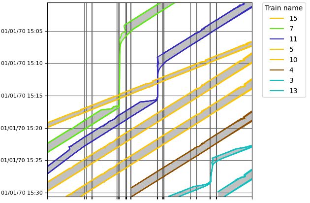
Selected solutions were validated using the simulation software D BB S IM, which is also
developed in the Digital Rail for Germany project. The simulation is a microscopic high-
speed simulation that can work with the same physics and safety model that were used in
the optimization model. Figure 11 shows a small selection of some trains and their braking
time slides provided from the simulation. The simulation was able to run the trains withns
e
computation tim
sub-MIP iteratio
requests routed
# competitions
# headways
# columns
algorithm
objective
scenario
# rows
25 BC 72131 62950 251 949 99 12674 132 22
25 MIP 93750 132566 21870 70565 99 12656 164 -
26 BC 53615 46559 51 134 96 41821 55 5
26 MIP 87151 155379 33587 108954 96 41824 138 -
27 BC 62318 55422 394 1689 98 22047 268 22
27 MIP 103956 185833 42032 132100 98 22052 331 -
28 BC 67691 60131 534 2333 98 22109 154 22
28 MIP 116989 220352 49832 162554 98 22109 607 -
29 BC 65606 58022 482 2357 97 32026 104 16
29 MIP 106167 190514 41043 134849 97 32021 319 -
30 BC 69835 62331 711 2976 96 42236 519 34
30 MIP 120702 227528 51578 168173 96 42236 1260 -
31 BC 63952 56050 536 2363 97 32001 307 22
31 MIP 107809 198118 44393 144431 97 32001 1077 -
32 BC 69365 63594 1114 5176 96 42079 515 39
32 MIP 127784 251287 59533 192869 96 42079 1597 -
33 BC 64235 56671 333 1747 98 22123 136 13
33 MIP 104467 188097 40565 133173 98 22120 300 -
34 BC 70436 65534 663 2959 97 32246 691 29
34 MIP 121210 239076 51437 176501 97 32247 1118 -
avg BC 65918 58726 507 2268 97 30136 288 22
avg MIP 108998 198875 43587 142417 97 30135 691 -
Table 5: Average and detailed results for test set HUNDRED.Figure 11: Time-space chart from the simulation D BB S IM.
only very minor deviations to the times and speed provided by the optimization solution
and without violations of the headway constraints.
7 Conclusion and Outlook
We developed a model formulation which is capable of routing and ordering trains under a
moving block regime. We provide a general timetabling definition GTTP which allows to
plug-in further details on the calculation of the running or headway time considered in the
model. This is done in an arranged way to construct a specially defined layered graph and
headway sets which are the basis of the presented MIP formulation.
An intended weakness of the model is clearly that the braking distance is only ensured at
supporting points in the network, i.e., at tails of the velocity arcs. For most cases this seems
to be sufficient, but of course it depends highly on the choice of κ. We see two options to
tackle this issue in the future. First, by refining the graph if in the simulation a critical point
on an edge is identified, or second, by extending the complexity of the headway callback.
In case of the larger instances (HUNDRED), we tested an iterative Sub-MIP-and-Cut
approach, which is already able to solve the problems faster than using pure MIP.
We are confident that the implementation of a classical Branch-and-Cut approach for
the headway constraints together with restart techniques and problem specific heuristics ap-
proaches can further improve the performance of the solving process. Hence, larger models
of GTTP can be solved to optimality or with a small optimality gap in the future.
Preliminary experiments indicate that considering more velocity levels does not change
the solution structure significantly. However, the approach is designed to refine the consid-
ered velocity levels of each request individually. Moreover, an adaptive way of constructing
the “right” levels during the solution process is clearly an open scientific topic. Note that
these levels do depend on the individual request as well as on other connected request in a
certain local neighborhood.
A huge potential in solving the timetabling and dispatching problem is also the combi-
nation with AI (Artificial Intelligence) methods, which are developed within the Digital Rail
for Germany program (Deutsche Bahn AG, 2019) and can produce solutions of good quality
very fast. The developed solver has already been used to validate the feasibility of generated
scenarios that are needed for a reinforcement learning approach. A future path of research
will be to analyze how the resulting recommendations from an reinforcement learning ap-
proach can be used as (partial) solutions to speed up the solver and how to develop furtherintegrated strategies. Acknowledgements We thank our colleagues from the simulation team at the Digital Rail for providing D BB S IM and the AI team for being an expert beta user of the developed solver. References Borndörfer, R., Klug, T., Lamorgese, L., Mannino, C., Reuther, M., and Schlechte, T., editors (2018). Handbook of Optimization in the Railway Industry, volume 268. Springer. Caprara, A., Fischetti, M., and Toth, P. (2002). Modeling and solving the train timetabling problem. Operations Research, 50(5):851–861. D’Ariano, A., Pacciarelli, D., and Pranzo, M. (2007). A branch and bound algorithm for scheduling trains in a railway network. European Journal of Operational Research, 183(2):643–657. Deutsche Bahn AG (2019). Digitale Schiene Deutschland – Die Zukunft der Eisenbahn. Available at https://digitale-schiene-deutschland.de/Downloads/ Brosch%C3%BCre_DigitaleSchiene_2019.pdf. Deutsche Bahn AG (2020). Infrastrukturzustands- und -entwicklungsbericht 2019. Avail- able at https://www.eba.bund.de/DE/Themen/Finanzierung/LuFV/ IZB/izb_node.html. Harrod, S. (2009). Capacity factors of a mixed speed railway network. Transportation Research Part E: Logistics and Transportation Review, 45(5):830–841. Harrod, S. S. (2012). A tutorial on fundamental model structures for railway timetable optimization. Surveys in Operations Research and Management Science, 17(2):85–96. Lamorgese, L. and Mannino, C. (2015). An exact decomposition approach for the real-time Train Dispatching problem. Operations Research, 63:48–64. Lamorgese, L. and Mannino, C. (2019). A noncompact formulation for job-shop scheduling problems in traffic management. Operations Research, 67(6):1586–1609. Mascis, A. and Pacciarelli, D. (2002). Job shop scheduling with blocking and no-wait constraints. European Journal of Operational Research, 143(3):498–517. Xu, P., Corman, F., Peng, Q., and X., L. (2017). A train rescheduling model integrating speed management during disruptions of high-speed traffic under a quasi moving block system. Transportation Research Part B, 104:638–666.
Appendix
traints
ions
# headway cons
requests routed
# competitions
sub-MIP iterat
# columns
algorithm
objective
scenario
runtime
# rows
1 BC 38128 34056 134 548 50 1346 51 7
1 MIP 47939 67873 9945 34365 50 1340 51 -
2 BC 31171 28053 67 225 49 11090 30 10
2 MIP 41048 57691 9944 29863 49 11094 41 -
3 BC 22332 19890 5 12 49 10838 22 2
4 MIP 29218 41006 6891 21128 49 10838 31 -
4 BC 30855 26478 21 51 49 10941 25 3
4 MIP 45188 73832 14354 47405 49 10941 50 -
5 BC 31822 28283 127 588 49 11004 33 10
5 MIP 48821 82759 17126 55064 49 11006 73 -
6 BC 32810 28820 104 516 49 11112 32 11
6 MIP 49026 79477 16320 51173 49 11105 73 -
7 BC 29000 25393 24 104 50 895 53 3
7 MIP 40964 61919 11988 36630 50 895 37 -
8 BC 29995 26345 91 400 49 10938 28 8
8 MIP 44345 72348 14441 46403 49 10938 46 -
9 BC 36328 32609 252 1119 50 1123 43 14
9 MIP 56009 96099 19933 64609 50 1123 106 -
10 BC 33680 30093 82 357 49 11033 45 7
10 MIP 48674 76911 15076 47175 49 11034 80 -
11 BC 30328 25722 40 186 49 10940 25 2
11 MIP 41205 61262 10917 35726 49 10940 43 -
12 BC 36397 32086 137 569 50 1223 34 8
12 MIP 55441 92681 19181 61164 50 1223 81 -
13 BC 32547 28893 246 1225 48 20995 71 25
13 MIP 45499 70289 13198 42621 48 20991 79 -
14 BC 27275 23596 23 58 49 10930 24 3
14 MIP 36406 52506 9154 28968 49 10931 39 -
15 BC 35410 31346 301 1417 50 1028 85 19
15 MIP 54094 92987 18985 63058 50 1029 105 -
16 BC 34763 31134 210 1094 48 20988 48 16
16 MIP 52786 88383 18233 58343 48 20985 68 -
17 BC 32453 28672 127 686 49 11050 26 6
17 MIP 49563 83473 17237 55487 49 11050 50 -
18 BC 32310 28355 118 664 50 1056 35 8
18 MIP 47844 79879 15652 52188 50 1056 78 -
19 BC 31548 27644 104 521 50 1013 35 11
19 MIP 43843 67740 12399 40617 50 1013 66 -
20 BC 41757 38515 675 2942 49 11141 264 24
20 MIP 67337 122400 26255 86827 49 11145 160 -
21 BC 39741 37213 626 2636 50 1316 352 26
21 MIP 62528 112559 23413 77982 50 1316 575 -
22 BC 31808 29121 154 775 49 10990 53 24
22 MIP 45653 77021 13999 48675 49 10986 76 -
23 BC 37459 35331 325 1464 49 11201 167 29
23 MIP 58240 103887 21106 70020 49 11202 97 -
24 BC 51496 48911 500 2209 50 1484 308 23
24 MIP 76212 131767 25216 85065 50 1492 127 -
Table 6: Detailed results for testset FIFTY.You can also read