MILIOM: Tightly Coupled Multi-Input Lidar-Inertia Odometry and Mapping
←
→
Page content transcription
If your browser does not render page correctly, please read the page content below

MILIOM: Tightly Coupled Multi-Input Lidar-Inertia
                                                                       Odometry and Mapping
                                                               Thien-Minh Nguyen, Member, IEEE, Shenghai Yuan, Muqing Cao, Lyu Yang,
                                                               Thien Hoang Nguyen, Student Member, IEEE and Lihua Xie, Fellow, IEEE

                                            Abstract— In this paper we investigate a tightly coupled                   Recently some researchers have started investigating the
                                         Lidar-Inertia Odometry and Mapping (LIOM) scheme, with the                 use of multiple 3D lidars for better coverage of the envi-
                                         capability to incorporate multiple lidars with complementary               ronment, especially in the field of autonomous driving [1]–
                                         field of view (FOV). In essence, we devise a time-synchronized
arXiv:2104.11888v1 [cs.RO] 24 Apr 2021

                                         scheme to combine extracted features from separate lidars into             [6]. In fact, though a single lidar mounted on the top of the
                                         a single pointcloud, which is then used to construct a local               vehicle can be cost sufficient, there are many scenarios where
                                         map and compute the feature-map matching (FMM) coeffi-                     the use of multiple lidars can be advantageous. For example,
                                         cients. These coefficients, along with the IMU preinteration               in some complex urban environments [1], [3], the combined
                                         observations, are then used to construct a factor graph that               FOV from multiple lidars provides a more comprehensive
                                         will be optimized to produce an estimate of the sliding window
                                         trajectory. We also propose a key frame-based map manage-                  observation of the surrounding, which allows the vehicle to
                                         ment strategy to marginalize certain poses and pointclouds in              navigate through the environment and avoid obstacles more
                                         the sliding window to grow a global map, which is used to                  flexibly. In a challenging subterranean scenario [2], where the
                                         assemble the local map in the later stage. The use of multiple             robot has to travel through some narrow and irregular terrains
                                         lidars with complementary FOV and the global map ensures                   that can cause the lidar’s FOV to be blocked, a multi-lidar
                                         that our estimate has low drift and can sustain good localization
                                         in situations where single lidar use gives poor result, or even            based localization technique was shown to be the solution to
                                         fails to work. Multi-thread computation implementations are                overcome such challenge.
                                         also adopted to fractionally cut down the computation time
                                         and ensure real-time performance. We demonstrate the efficacy
                                         of our system via a series of experiments on public datasets
                                         collected from an aerial vehicle.

                                                                 I. I NTRODUCTION
                                            Over the years, 3D lidars have proved to be a reliable
                                         and accurate localization solution for autonomous systems.
                                         Compared with the other class of onboard self-localization
                                         (OSL) based on camera, lidar clearly possesses many su-
                                         perior characteristics. In terms of sensing capability, lidar
                                         can provide 360 degree observation of the environment, with
                                         metric-scaled features, while the best fisheye cameras still
                                         only have up to 1800 field of view (FOV), and can only                     Fig. 1: Illustration of the localization drift by using single
                                         extract features of unknown scale. Even when compared to                   lidar in a challenging environment.
                                         multi-camera or RGBD camera systems, which are supposed
                                         to solve the scale problem, lidar still has a much higher sens-               In the aforementioned works, we note that lidar was used
                                         ing range, is almost unaffected by lighting conditions, and                mostly on ground robots operating in 2D space, hence it is
                                         requires very little calibration effort. Nevertheless, high cost           usually assumed that the ground plane can be observed most
                                         and weight has been one of lidar’s main weaknesses, and has                of the time. This is no longer the case with aerial robots,
                                         mostly restricted its application to ground robot platforms.               which is the targeted application of this work. Fig. 1 gives
                                         However, in recent years, both the cost and weight factors                 an example of such a scenario, in which, there are two lidars
                                         have been significantly reduced thanks to many technological               mounted on an Unmanned Aerial Vehicle (UAV), and the
                                         innovations. Hence, we have observed an uptick of 3D lidar                 only nearby objects that can be observed are the building
                                         applications in the robotics community.                                    facade and the ground. Hence with a single horizontal lidar,
                                                                                                                    a commonly known Lidar Odometry and Mapping (LOAM)
                                            This work was partially supported by the Wallenberg AI, Autonomous
                                         Systems and Software Program (WASP) funded by the Knut and Alice Wal-
                                                                                                                    method1 gives the result that expectedly drifts in the vertical
                                         lenberg Foundation, under the Wallenberg-NTU Presidential Postdoctoral     direction (blue path in Fig. 1), as it cannot observe the
                                         Fellowship Program. (Corresponding author: Thien-Minh Nguyen)              ground. Similarly, when using the vertical lidar, the result
                                            The authors are with School of Electrical and Electronic Engineering,
                                         Nanyang Technological University, Singapore 639798, 50 Nanyang
                                                                                                                    exhibits significant drift in the lateral direction (orange path
                                         Avenue. (e-mail: thienminh.nguyen@ntu.edu.sg, shyuan@ntu.edu.sg,           Fig. 1), as it lacks observations to counter drift in that
                                         mqcao@ntu.edu.sg,       lyu.yang@ntu.edu.sg,     e180071@e.ntu.edu.sg,
                                         elhxie@ntu.edu.sg)                                                           1 https://github.com/HKUST-Aerial-Robotics/A-LOAM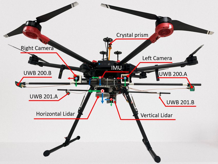
direction. In this work our main goal is to show that when           and provide accurate estimate, thanks to the use of multi-
these lidars are combined in a tighly coupled manner, the            thread implementation and low programming overheads.
challenge can be effectively overcome.                                  The main contribution of this work can be listed as
                                                                     follows:
                    II. R ELATED W ORKS                                 • We propose a general scheme to combine multiple li-
                                                                          dars with complementary FOV for feature-based Lidar-
   Many 3D lidar-based localization methods have been pro-                Inertia Odometry and Mapping (LIOM) application.
posed in the last decade. Most notable is the work by Zhang             • We propose a tightly-coupled, key frame-based, multi-
et al [7], [8]. In [7], the authors proposed a standard frame-            threaded multi-input LIOM framework to achieve robust
work for lidar-based odometry and mapping. Indeed, their                  localization estimate.
technique to calculate smoothness and determine plane and               • We demonstrate the advantages of the method over
edge features from lidar scans remains a popular approach                 existing methods via extensive experiments on an ad-
that is still widely adopted to this day. In [8], the authors pro-        vanced UAV platform.
posed a loosely coupled lidar-visual-inertial localization and          The remainder of the paper is organized as follows: in
mapping system, which was also demonstrated to work on               Sec. III, we lay out the basic definitions, notations and for-
a UAV. However, several techniques used in this work seem            mulations of the problem; Sec. IV then presents an overview
to be no longer efficient compared to current state-of-the-          of the software structure and the flow of information. Sec.
art. For example, the edge and plane features have separate          V and Sec. VI discuss in details how lidar data and IMU
factors with high non-linearity, while in recent works, it has       are processed. Next we describe the construction of the
been shown that one edge factor can be substituted by two            local map and the feature-to-map matching (FMM) process
plane factors [3], [9] with relatively simpler formulation. In       that produces the FMM coefficients for constructing the
addition, the voxel-based map management scheme appears              lidar factors. Sec. VIII explains the key frame management
to be quite complex. In contrast, inspired by contemporary           procedures. We demonstrate the capability of our method via
VIO frameworks, in this work we propose a more efficient             several experiments on UAV datasets in Sec. IX. Finally, Sec.
framework based on so-called key frame, which simplifies             X concludes our work.
the query as well as update on the map.
                                                                                         III. P RELIMINARIES
   Besides, to the best of our knowledge, few works have
satisfactorily investigated the tight coupling of IMU prein-         A. Nomenclature
tegration factors with lidar factors in the literature, despite         In this paper we use (·)> to denote the transpose of an
its extensive applications in visual-inertial systems [10]–[14].     algebraic vector or matrix under (·). For a vector x ∈ Rm ,
                                                                                                                    2
In [15], a method based on this idea was proposed, however           kxk stands for its Euclidean norm, and kxkG is short-hand
                                                                              2
the lidar processing part assumes the presence of distinct           for kxkG = x> Gx. For two vectors v1 , v2 , v1 ×v2 denotes
planes that can be extracted via RANSAC in the environ-              their cross product. In later parts, we denote R ∈ SO(3) as
ments. In [16], a tightly-coupled framework called LIO-              the rotation matrix, and T ∈ SE(3) as the transformation
Mapping was proposed. Inspired by the VIO frameworks,                matrix. We denote Q as the set of unit quaternions, with
both of the aforementioned works use a sliding window, and           q as its identity element. Given q ∈ Q, R(q) denotes
employ IMU preintegration and lidar features to construct            its corresponding rotation matrix, and vec(q) returns its
cost factors that couple the measurements with the robot             vector part. Also, in the later parts, we refer to the mapping
poses in the sliding window. Later, Shan et al. released             E : R3 7→ Q and its inverse E −1 : Q → R3 to convert a
the LIO-SAM package [16] which optimizes a pose graph                rotation vector, i.e. the angle-axis representation of rotation,
leveraging IMU preintegration and pose priors as the cost            to its quaternion form, and vice versa. The formulae for these
factors. Unfortunately, LIO-Mapping performs very poorly             operations can be found in [12].
when forced to run in real-time, which is also reported in              When needed for clarity, we attach a left superscript to
other works [2], [9], [17]. We believe this is due to several        an object to denote its coordinate frame. For example A v
inefficient implementation designs. On the other hand, LIO-          implies the coordinate of the vector v is in reference to the
SAM requires 9DoF IMU, and should be better categorized              frame A, and B F indicates that the coordinate of the points in
as a loosely coupled method, as it uses pose priors that             the pointcloud F is w.r.t. to the frame B. A rotation matrix
are obtained from a LOAM process with a separate LM-                 and transformation matrix between two coordinate frames
based optimization process proposed earlier [18], instead of         are denoted with the frames attached as the left-hand-side
jointly optimizing the lidar feature and IMU preintegration          superscript and subscript, e.g., AB R and AB T are called the
factors together. Besides, we also note that the aforemen-           rotation and transform matrices from frame A to B, respec-
tioned works do not generalize to multi-lidar case, which            tively. When the coordinate frames are the body frame at
poses a new challenge as it requires us to design a stable           different times, depending on the context, we may omit and
synchronization scheme, as well as a time-efficient frontend         rearrange the superscript and subscripts to keep the notation
to ensure real-time performance. As will be shown later,             concise, e.g., k Rk+1 , BBkk+1 R, or w      Bw
                                                                                                           m T , Bm T.
despite integrating multiple lidars, and employing tightly              Throughout this paper we define a local frame L whose
coupled scheme, our method can still operate in real-time            origin coincides with the position of the body frame at the
Whenever the context requires, we can make the notation
                                                 L #»                         more explicit.
                                                  z
                                  L               B0    #»
                                                        y         L #»           The inputs of the system are the IMU measurements,
                                  Bw T                             y
                      L                                                       i.e. acceleration at and angular velocity ωt , and lidar
                      Bj T                                          B0   #»                             i
                                                                         x    raw pointclouds Pm          . The outputs are the optimized esti-
                                                                    L #»      mates of the sliding window state estimates, denoted as
                    L                                                    x
                    Bk T                                                      {X̂w , X̂w+1 , . . . , X̂k }, and the IMU-predicted state estimate
                                                                              up to time t, denoted as X̂t .
                                            #»        B0     #»
                                                             z
                                            g                                             ωt ,
                                                                                          at                              Ik                 X̂t
Fig. 2: The local frame L defined via the initial body frame
B0 , and the poses of the robot at later time instances.
                                                                                           i
                                                                                          Pm
                                                                                                           F̆k

initial time, denoted as B0 . In addition, the L #»      z axis of L L
points towards the opposite direction of the gravity vector #»                                                                       {. . . Lim }
                                                                             L             L
                                                                    g { Fw , Fw+1 , . . . , Fk }
(see Fig. 2), its L #»
                                                                                                                    Mw
                      x axis points to the same direction of the
                 B0 #»                                      L #»
projection of x on a plane perpendicular with z axis,
and the L #»
           y axis can be determined by the right-hand rule.                                             {X̂w , X̂w+1 , . . . , X̂k }

Indeed, these calculations can be done by simply using the Fig. 3: Main processes and available quantities in the system
initial acceleration reading from the IMU, which contains by the time t. Note that lines of different colors are not
only the coordinate of the vector #»      g in B0 , to determine the connected.
pitch and roll angles of B0 with respect to L, assuming that
the error due to acceleration bias is negligible.                         In the above framework, the joint optimization process
B. State estimates                                                     consumes      the most computation time, while most other
                                                                       processes are meant to extract the key information used
   In reference to Fig. 2, we define the robot states to be
                                                                       for constructing the factors that will be optimized in the
estimated at time tk as:
                                                                     following cost function:
                                             ω    a
                 Xk = qk , pk , vk , bk , bk ,                     (1)                (      k
                                                                                             X                                 2
                                                                           f (X̂ ) ,              rI (X̂m−1 , X̂m , Im ) −1
                                 3           3
where qk ∈ Q, pk ∈ R , vk ∈ R are respectively the                                         m=w+1
                                                                                                                               PIm

orientation quaternion, position and velocity of the robot                                   k |Cm|
                                                                                                                                     !)
                                                                                                                               2
w.r.t. the local frame L at time tk ; bak , bω            ∈      3                           X   X
                                                       k       R   are                  +           ρ                 i
                                                                                                         rL (X̂m , Lm ) −1                  , (4)
respectively the IMU accelerometer and gyroscope biases.                                                                       P i
                                                                                            m=w i=1                              Lm

Hence, we denote the state estimate at each time step k, and
                                                                       where rI (·) and rL (·) are the IMU and lidar residuals, ρ(·)
the sliding window of size M as follows:
                                                                     is the Huber loss function to suppress outliers, PIm and
                                   ω   a
     X̂k = q̂k , p̂k , v̂k , b̂k , b̂k ,                           (2) PLim are the covariance matrix of their measurements, Im
                                                                     and Lm are respectively IMU preintegration and lidar FMM
     X̂ = X̂w , X̂w+1 , . . . , X̂k , w , k − M + 1.               (3) coefficients, Cm denotes the set of FMM features derived
                                                                       from the lidar feature cloud at time tm . Note that each IMU
Note that in this work we assume the extrinsic parameters factor in (4) is coupled with two consecutive states, while
have been manually calibrated, and each lidar’s pointcloud each lidar factor is coupled with only one. In this paper,
has been transformed to the body frame before being pro- the IMU factors are calculated via an integration scheme as
cessed further. Moreover, depending on the context we may described in our previous work [12]. Hence we only recall
also refer to R̂k , R(q̂k ) as the rotation matrix estimate, some important steps due to page constraints. In the next
and (R̂k , p̂k ) or (q̂k , p̂k ) as the pose estimate.                 sections we will elaborate on the processing of lidar and
                  IV. G ENERAL F RAMEWORK                              IMU data for use in the optimization of (4).
   Fig. 3 presents a snapshot of our MILIOM system at some                                       V. L IDAR PROCESSING
IMU sample time t past tk , where tk is the start time of the                    Fig. 4 presents an illustration of the synchronization be-
skewed combined feature cloud (SCFC) F̆k (more details are                    tween the lidars. Specifically, for a lidar i, we can obtain
given in Sec. V). Indeed, there are two types of features that                a sequence of pointclouds Pm    i
                                                                                                                , each corresponds to a 3D
can be extracted from the lidar scans, namely edge feature                    scan of the environment over a fixed period (which is around
and plane feature. Thus when we refer to a feature cloud F,                   0.1s for the Ouster2 sensor used in this work). We assume
we do mean the compound F , (F e , F p ), where F e is
the set of edge features, and F p is the set of plane features.                 2 https://ouster.com/products/os1-lidar-sensor/
that lidar 1 is the primary unit, whose start times are used feature extraction, the ring by ring structure will be lost and
to determine the time instances of the state estimates on one cannot trace the smoothness of the points on the ring
the sliding window, and others are referred to as secondary to extract feature. On the other hand, LOCUS uses General
lidars. Each pointcloud input is put through a feature ex- Iterative Closest Point (GICP) for scan matching, which does
traction process using the smoothness criteria as in [7] to not concern features, however it requires good IMU and/or
obtain the corresponding feature cloud. We then merge all wheel-inertial odometry (WIO) information for initial guess
feature clouds whose start times fall in the period [tk−1 , tk ) of the relative transform between the two pointclouds.
to obtained the SCFC F̆k .
VI. IMU P ROCESSING
1
Pm
2
In Fig. 5, we illustrate the process of synchronizing
Pm
n
the IMU data with the lidar pointcloud. Recall that t0k
Pm
is the end time of the last SCFC, and that during the
F̆w
period [tk−1 , t0k ), we obtain the following IMU samples
{(ωτm , aτm ), (ωτm+1 , aτm+1 ), . . . , (ωτN 0 , aτN 0 )}. These
F̆w+1
samples will be used for two operations below.
...
LF
F̆k w
LF
tw ... tk−1 tk t0k w+1
LF
Fig. 4: Illustration of the feature extraction and synchroniza- k−1
tion between the lidar scans. Assuming that there are n lidars, F̆k
i
Pm refers to the pointclouds of lidar i ∈ {1, 2, . . . , n}. Note
IMU
that F̆k is the last SCFC that comes out from the feature
extraction and synchronization block with the start time tk Preintegration Propagation
and the end time t0k . tw ... tk−1 tk t0k
Fig. 5: Synchronization between the CFC and the IMU. The
Note that if the scan period of a lidar is 0.1s, then a light blue circles represent the interpolated samples at the
SCFC can stretch over a maximum of 0.2s period. This is start and end times of the CFCs.
a significant time-span where the robot motion can affect
the pointcloud in the scan, however since all of the points
in the pointclouds are timestamped, we can use the IMU- A. Preintegration
based state propagation to compensate for the robot motion, First, we use the samples in the sub-interval [tk−1 , tk ) to
which we refer to as the ”deskew” process. Specifically, for calculate the so-called preintegration observations using the
a feature point Bts f in the SCFC F̆k stretching over the time zero-order-hold (ZOH) technique:
span [tk , t0k ), its coordinates w.r.t. the robot’s pose at time
tk can be calculated by the interpolation:
γ̆ τm+1 = γ̆ τm ◦ E (∆τm ω̄τm ) , (6a)
β̆ τm+1 = β̆ τm + ∆τm R(γ̆ τm )āτm , (6b)
Bts
f , R slerp q, ttk0 q̆, s Bts f + sttk0 p̆,
(5)
k k 2
∆τm
ᾰτm+1 = ᾰτm + ∆τm β̆ τm + 2 R(γ̆ τm )āτm , (6c)
ts
where s = and slerp(q1 , q2 , s) is the spherical linear
t0k −tk
interpolation operation on quaternions [19], ttk0 q̆ and ttk0 p̆ γ̆ τ0 , q, β̆ τ0 , 0, ᾰτ0 , 0, (6d)
k k
are the orientation and position of Bt0k w.r.t. Btk . More
ω̄τm , (ωτm − b̂ω a
k−1 ), āτm , (aτm − b̂k−1 ),
(6e)
information on the IMU propagation is given in Sec. VI-B.
After deskew, a SCFC F̆m becomes B Fm , the so-
∆τm , τm+1 − τm , m ∈ {0, 1, . . . , N }, (6f)
called deskewed combined feature cloud, or simply
τ0 = tk−1 , τN +1 = tk , (6g)
CFC for short. We further use the state estimates
where ◦ is the quaternion product, and E(·) is the mapping
{X̂w , X̂w+1 , . . . , X̂k−1 } and the IMU-propagated states q̆k ,
from rotation vector to quaternion described in Sec. III.
p̆k (see Fig. VI-B) to transform {B Fw , B Fw+1 , . . . , B Fk } to
At the end of the preintagration process (6), we can obtain
{L Fw , L Fw+1 , . . . , L Fk }, which are employed in the con-
the preintegration observations Ik , (ᾰtk , β̆ tk , γ̆ tk ). The
struction of the local map and the FMM process in Sec. VII.
use of this observation in an optimization framework has
Remark 1. Our synchronization scheme differs from LOCUS been described in depth in our previous work [12], and we
[2] in that the merging of the pointclouds is made on full-size refer to that for more details.
poinclouds in [2], while ours is made on feature pointclouds.
The reason for choosing this merging scheme is because the B. State Propagation
feature extraction part is done on distinct rings, using the Given the IMU samples over [tk−1 , t0k ) and the state
information on the horizontal and vertical angular resolution estimate X̂k−1 , we propagate the state further in time and
of the lidar sensors. Hence if the merging happens before the obtain the IMU-predicted poses at time tk and t0k , denoted
as (p̆k , q̆k ) and (p̆t0k , q̆t0k ), for the deskew of the SCFC. The compute the Hesse normal vectors of the two planes, one
propagation is done using the ZOH technique as follows: that goes through this line and f , and another that also goes
through the edge line but is perpendicular to the first plane.
q̆τm+1 = q̆τm ◦ E (∆τm ω̄τm ) , (7a) Hence, we compute the fitness score to decide whether to
v̆τm+1 = v̆τm + ∆τm [R(q̆τm )āτm − g] , (7b) add the tuples (m f i , g n̄1 , gc1 ) and (m f i , g n̄2 , gc2 ) to the set
Cm . Fig. 6 illustrates the vectors and planes computed over
p̆τm+1 = p̆τm + ∆τm v̆τm . . .
these steps.
(∆τm )2
+ [R(q̆τm )āτm − g] , (7c) It should be noted that the FMM process can be quite
2 computationally expensive. However, since Algorithm 1 does
q̆τ0 = q̂k−1 , v̆τ0 = v̂k−1 , p̆τ0 = p̆k−1 , (7d) not modify the local map, the FMM process can be split into
0
∆τm , τm+1 − τm , m ∈ {0, 1, . . . , N, . . . , N }, (7e) multiple threads for each CFC. Thanks to this strategy, we
can cut down the computation time to about 10m to 20ms
τ = t
0 k−1 , τN +1 = tk , τN 0 +1 = t, (7f)
compared to hundreds of ms when using a single thread.
where we reuse the definition of ω̄τm and āτm in (6e).
Hence we obtain the relative transform from time tk to
Algorithm 1: Calculation of FMM coefficients
t0k by ttk0 q̆ , q̆−1 tk −1
tk q̆t0k and t0k p̆ , −R(q̆tk )(q̆t0k − q̆tk ). This
p e
k
transform is used for the deskew of the SCFC in Sec. V. Input: Fm = (Fm , Fm ), Mw = (Mpw , Mew ), T̂m .
Output: Cm , {Lm , Lm , . . . , }, Lim , (m f i , ni , ci ).
1 2
Remark 2. It might be useful to note the difference between 1 for each f ∈ Fm do
IMU propagation and IMU preintegration. On the physical 2 Compute m f i from f i and T̂m ;
sense, IMU propogation uses IMU measurement to project 3 if f ∈ Fmp
then
the system’s state from time tk to time t, while preintegration 4 Find Nf = KNN(f ,PMpw );
is the direct integration of IMU measurements to obtain some > 2
pseudo-observation [20]. In a technical sense, preintegration
5
n x∈N>f ||n x + 1|| ;
Find n̄ = argmin
|n̄ f +1| s
does not involve cancelling the gravity from the accelera- 6 Compute s = 1 − 0.9 kn̄kkf k and g = kn̄k ;
tion measurement before integration (when comparing (6b),
7 If s > 0.1, add (m f i , g n̄, g) to Cm ;
(6c) with (7b), (7c)), nor does it require the initial state e
8 else if f ∈ Fm then
(q̂k−1 , v̂k−1 , p̆k−1 ) (when comparing (6d) with (7d)).
9 Find the set Nf = KNN(f , Mew ), and its
1
P
VII. L OCAL M AP AND FMM P ROCESSES centroid p̄ = |Nf | x∈Nf x;
Compute: A , |N1f | x∈Nf (x − p̄)(x − p̄)> ;
P
The local map Mw is used as a prior map to calculate 10
the FMM coefficients for the joint optimization process. In 11 Find the eigenvector vmax corresponding to
the beginning, when fewer than M key frames have been the largest eigenvalue of A;
stored to the memory, we directly merge the CFCs of the 12 Compute: x0 = f , x1 = p̄ + 0.1vmax ,
first M − 1 steps obtained in Sec. V to obtain Mw . On the x2 = p̄ − 0.1vmax , v01 = x0 − x1 ,
other hand, when enough key frames have been created, we v02 = x0 − x2 , v12 = x1 − x2 , ;
will use the latest IMU-predicted state estimate p̆k to search 13 Compute: n1 = v12 × (v10 × v02 ),
for the M nearest key frames, and merge the corresponding n1 ← n1 / kn1 k, n2 = v12 × n1 ;
pointclouds to obtain Mw . 14 Compute: f ⊥ = f − (n1 n> 1 )v01 ;
Next, for each CFC L Fm , m = w, w + 1, . . . , k, we 15 Compute: c1 =h−n> 1 ⊥f and c2 =i −n>2 f ⊥;
calculate the FMM coefficients for each of its features by 0.9kx01 ×x02 k
16 Compute: s = 1 − kx12 k , g = s/2;
using Algorithm 1. In steps 3-7 of this algorithm, for each m i
17 If s > 0.1, add ( f , g n̄1 , gc1 ) and
plane feature f we find a set Nf of neighbouring plane
(m f i , g n̄2 , gc2 ) to Cm ;
features in the local map using KNN, then calculate the
18 end
Hesse normal n of a plane, whose sum of squared distances
to the points in Nf is minimal (this optimization problem has
closed-form solution). We then calculate the ”fitness score” s The result of the FMM is a list of coefficients used to
in step 6. If the fitness score is above a threshold in, we can create a lidar factor in (4). Specifically, for each tuple of
admit the tuple (m f i , g n̄, g) to the set of FMM coefficients FMM coefficients Lim = (m f i , ni , ci ), we can calculate the
of CFC Fm , denoted as Cm . corresponding residual as follows:
For steps 8-17, we follow a similar procedure to calculate
rL (X̂m , Lim ) = (ni )> R(q̂m )m f i + p̂m + ci . (8)
the coefficients of an edge feature. Our strategy here is to
construct the two planes that intersect at the presumed edge Remark 3. Note that both L Fm and Mw in Algorithm 1
line, as such, if f belongs to the edge line, it belongs to both are w.r.t. to the L frame, thus we omit the superscript for
of these planes and vice versa. To find the edge line, we more concise notation. Also, either Mw or Fm or both
find the fittest line going through the neighbor set Nf and can be down-sampled to reduce the computational load. In
its centroid p̄, which corresponds to steps 9-11. From step this paper we chose a 0.4m leaf size for the plane feature
12 to step 15, using some geometrical manipulations, we pointclouds and 0.2m for the edge feature pointclouds.Fig. 6: Illustrations of the vectors and the two planes com-
puted in step 12 to step 15 of Algorithm 1.
Fig. 7: Hardware setup of the viral dataset, with one hor-
izontal and one vertical lidar whose fields of view are
VIII. K EY FRAME M ANAGEMENT complementary.
.
The key frame in this case refers to marginalized pose es-
timates, so-called key poses, and their corresponding CFCs,
so-called key pointclouds. After each joint optimization can scan the front, back, left, right, while the vertical lidar
step, we will consider admitting the middle pose estimate, can scan the front, back, above and below sides of the UAV.
i.e. (q̂v , p̂v ), v , k − M/2 to the list of key poses. Both lidars have 16 channels with 32o vertical FOV.
Specifically, given p̂v , we will find its KNN among the We compare our algorithms with the two latest LIO based
key poses and create the sets Np = {p0 , p1 , . . . , pK } methods, which is LIO-Mapping [16] (henceforth referred
and Nq = {q0 , q1 , . . . , qK } that contain the positions and to as LIO-M) and LIO-SAM [9], and the MLOAM4 [3]
quaternions of these key poses, respectively. Hence, we check method, which integrates multiple lidars but does not employ
the following: IMU measurements. We note that both LIO-M and LIO-SAM
• kp̂v − pk > 1.0, ∀p ∈ Np , are designed for single lidar configuration. More specifically,
• E −1 (q̂−1v q) > π/18, ∀q ∈ Nq , they assume the pointcloud input to be of regular shape and
where E −1 is the inverse of E, which returns the rotation use the vertical and angular steps to extract the pointcloud
vector from a quaternion. If either one of the two conditions features. In theory, we can modify their code to replace the
above is true, then we will admit this pose estimate to the internal feature extraction process with our feature extraction
list of key poses and save its corresponding CFC Fv to the & merging part (Fig. 3) and inject the CFC into their back-
buffer for later use in the construction of local map. end. However this would involve too much modification into
the original code structure. Therefore, we opt to configure our
IX. E XPERIMENT method as well as the others to work with a single horizontal
In this section we describe our implementation of the lidar and report the result in Tab. I. We then configure our
MILIOM method and seek to demonstrate its effectiveness method to work with both lidars and append the result to
through a series of experiments on UAV datasets. The soft- Tab. I. The details of these configurations will be provided
ware system is developed on the ROS framework, employs on the NTU VIRAL dataset’s website.
the ceres-solver for the joint optimization process and other All parameters such as the standard deviation of IMU
libraries such as PCL, Eigen, etc for their utilities. All noises, window size, downsampling resolution, etc., are kept
experiments were done on a core-i7 computer with 6 cores. uniform. All methods are required to run at the full lidar
Video recording of some experiments can be viewed at rate, which is 10 Hz. However, for LIO-M, we reduce the
https://youtu.be/dHXYWC2KJyo. rate of the lidar topic to one third of the actual rate (10
Hz) to allow the algorithm to run in real-time. Even with
A. NTU VIRAL Datasets this we also have to limit the time for the optimization
We employ our recently published NTU VIRAL dataset process when the buffered data becomes too large. We run
[21]3 , which to the best of our knowledge is the first each algorithm on each dataset once and record the IMU-
UAV dataset that contains data from multiple lidars (besides predicted estimates. The estimated and grountruth trajectories
multiple cameras, IMUs, Ultra-wideband (UWB) ranging are then synchronized and aligned with each other. The
sensors). The configuration of the two lidars can be seen resulting Absolute Trajectory Error (ATE) of each test and
in Fig. 7. More specifically, one so-called horizontal lidar each method is computed and reported in Tab. I. These
3 https://ntu-aris.github.io/ntu_viral_dataset/ 4 https://github.com/gogojjh/M-LOAMTABLE I: ATE of the lidar-based localization methods over
the NTU VIRAL datasets. The best result is highlighted in
bold, the second best is underlined. All values are in m.
Dataset 1-Lidar 2-Lidar
LIO-M LIO-SAM Ours MLOAM Ours
eee 01 1.0542 0.0915 0.1042 0.1945 0.0666
eee 02 0.7234 0.0815 0.0650 0.2996 0.0656
eee 02 1.0314 0.1176 0.0628 0.1555 0.0518
nya 01 2.2436 0.0899 0.0832 0.2334 0.0565
nya 02 1.9664 0.1068 0.0721 0.2859 0.0668
nya 03 2.9934 0.3655 0.0577 0.1925 0.0423
sbs 01 1.6737 0.0966 0.0764 0.1925 0.0658
sbs 02 1.8056 0.0961 0.0806 0.1778 0.0816
sbs 03 2.0006 0.0960 0.0884 0.1863 0.0933
Fig. 9: Visualization of the trajectory estimate by MIL-
IOM method (blue line), ground truth (red line), key frame
positions (yellow circles), activated key frames used for
constructing the local map (light green), and the global map
built by merging all of the key pointclouds. This experiment
is done over the sbs 03 dataset.
arrived at the buffer.
Fig. 8: Error of the estimates by different methods on the
eee 02 dataset.
Fig. 10: Computation times of the main MILIOM processes
in eee 02 dataset: ∆tloop is the time period between the
tasks are done by the matlab scripts accompanying the NTU beginning of one joint optimization process to the next,
VIRAL data suite [21]. ∆tbackend is the time for the ceres-solver to actually solve the
It is clearly shown in Tab. I that our system consistently joint optimization problem (4), ∆tfrontend is the computation
achieves better performance compared to existing methods, time for all of the preliminary processes including deskew,
as MILIOM with a single lidar already performs better transform and FMM processes before the optimization starts.
than other methods, including multi-lidar MLOAM method.
When configured to work with both lidars, the result is also
consistently improved compared to the single lidar case. B. Building Inspection Trials
In Fig. 8, we can observe a maximum error of 10cm by We also conduct several trials to test the ability of the
MILIOM method with two lidars. We also visualize our method in actual inspection scenarios, one of which was
mapping and key frame management schemes in Fig. 9. shown earlier in Fig. 1. Indeed, these operations can be
Fig. 10 reports the computation time for the main pro- more challenging than the NTU VIRAL datasets for several
cesses when running the eee 02 dataset. The frontend pro- reasons. First, there are only a building facade and the ground
cessing time, which is mainly consumed by the FMM pro- plane where reliable features can be extracted. Second, the
cess, has a mean of 14.56 ms. While the backend processing building is much taller than the structures in the NTU
time, dominated by the optimization time of the ceres solver, VIRAL datasets, and when flying up to that high, there
has a mean of about 62.9902 ms. The mean of the loop might be very few features that can be extracted. Finally, the
time is 99.99 ms, which exactly matches the lidar rate. The trajectory of the UAV is mostly confined to the YZ plane,
fluctuation in ∆tloop is reflective of the soft synchronization instead of having diverse motions as in the NTU VIRAL
scheme when sometimes we have to wait for some extra datasets. Hence there can be some observability issues with
time for data from all lidars to arrive, and sometimes we can the estimation.
immediately start on new frontend processing task when the Tab. II summarizes the results of these inspection trials.
current backend completes just when all lidar inputs have In general, the aforementioned challenges do increase theTABLE II: ATE of the lidar-based localization methods on R EFERENCES
some object inspection trials. The best result is highlighted
[1] J. Jeong, Y. Cho, Y.-S. Shin, H. Roh, and A. Kim, “Complex
in bold, the second best is underlined. All values are in m. urban dataset with multi-level sensors from highly diverse urban
environments,” The International Journal of Robotics Research, p.
Dataset 1-Lidar 2-Lidar 0278364919843996, 2019.
LIO-M LIO-SAM Ours MLOAM Ours [2] M. Palieri, B. Morrell, A. Thakur, K. Ebadi, J. Nash, A. Chat-
test 01 3.6611 - 2.2460 3.9609 0.2524 terjee, C. Kanellakis, L. Carlone, C. Guaragnella, and A.-a. Agha-
test 02 5.0644 - 2.0184 0.6699 0.3378 mohammadi, “Locus: A multi-sensor lidar-centric solution for high-
test 03 5.7629 - 4.4470 3.4921 0.1444 precision odometry and 3d mapping in real-time,” IEEE Robotics and
Automation Letters, vol. 6, no. 2, pp. 421–428, 2020.
[3] J. Jiao, H. Ye, Y. Zhu, and M. Liu, “Robust odometry and mapping for
multi-lidar systems with online extrinsic calibration,” arXiv preprint
arXiv:2010.14294, 2020.
[4] J. Geyer, Y. Kassahun, M. Mahmudi, X. Ricou, R. Durgesh, A. S.
Chung, L. Hauswald, V. H. Pham, M. Mühlegg, S. Dorn et al., “A2d2:
Audi autonomous driving dataset,” arXiv preprint arXiv:2004.06320,
2020.
[5] S. Agarwal, A. Vora, G. Pandey, W. Williams, H. Kourous, and
J. McBride, “Ford multi-av seasonal dataset,” The International Jour-
nal of Robotics Research, vol. 39, no. 12, pp. 1367–1376, 2020.
[6] P. Sun, H. Kretzschmar, X. Dotiwalla, A. Chouard, V. Patnaik, P. Tsui,
J. Guo, Y. Zhou, Y. Chai, B. Caine et al., “Scalability in perception
for autonomous driving: Waymo open dataset,” in Proceedings of the
IEEE/CVF Conference on Computer Vision and Pattern Recognition,
2020, pp. 2446–2454.
[7] J. Zhang and S. Singh, “Loam: Lidar odometry and mapping in real-
time.” in Robotics: Science and Systems, vol. 2, no. 9, 2014.
[8] ——, “Laser–visual–inertial odometry and mapping with high robust-
ness and low drift,” Journal of Field Robotics, vol. 35, no. 8, pp.
1242–1264, 2018.
[9] T. Shan, B. Englot, D. Meyers, W. Wang, C. Ratti, and R. Daniela,
“Lio-sam: Tightly-coupled lidar inertial odometry via smoothing and
Fig. 11: Visualization of the result in on the building inspec- mapping,” in IEEE/RSJ International Conference on Intelligent Robots
tion test 01. and Systems (IROS). IEEE, 2020.
[10] C. Forster, L. Carlone, F. Dellaert, and D. Scaramuzza, “On-manifold
preintegration for real-time visual–inertial odometry,” IEEE Transac-
error for all methods. We couldn’t get LIO-SAM to work tions on Robotics, vol. 33, no. 1, pp. 1–21, 2016.
[11] T. Qin, P. Li, and S. Shen, “Vins-mono: A robust and versatile monoc-
in these datasets till the end without divergence. Even for ular visual-inertial state estimator,” IEEE Transactions on Robotics,
the MILIOM method with a single lidar, there is also a vol. 34, no. 4, pp. 1004–1020, 2018.
significant increase in the error. On the other hand, contrary [12] T.-M. Nguyen, M. Cao, S. Yuan, Y. Lyu, T. H. Nguyen, and L. Xie,
“Viral-fusion: A visual-inertial-ranging-lidar sensor fusion approach,”
to its lower performance over NTU VIRAL datasets, in these Submitted to IEEE Transactions on Robotics, 2021.
challenging building inspection trials, MLOAM can take [13] T. H. Nguyen, T.-M. Nguyen, and L. Xie, “Tightly-coupled single-
advantage of complementary FOVs of both lidar, thus achiev- anchor ultra-wideband-aided monocular visual odometry system,” in
2020 IEEE International Conference on Robotics and Automation
ing significantly higher accuracy than single-lidar MILIOM. (ICRA). IEEE, 2020, pp. 665–671.
Nevertheless, the results of the two-lidar MILIOM approach [14] ——, “Range-focused fusion of camera-imu-uwb for accurate and
are still most accurate, which demonstrates the robustness drift-reduced localization,” IEEE Robotics and Automation Letters,
vol. 6, no. 2, pp. 1678 – 1685, 2021.
and accuracy of the multi-input lidar-inertia approach in [15] P. Geneva, K. Eckenhoff, Y. Yang, and G. Huang, “Lips: Lidar-
critical conditions. Fig. 11 presents the 3D plot of the inertial 3d plane slam,” in 2018 IEEE/RSJ International Conference
trajectory estimates, the global map and groundtruth in one on Intelligent Robots and Systems (IROS). IEEE, 2018, pp. 123–130.
[16] H. Ye, Y. Chen, and M. Liu, “Tightly coupled 3d lidar inertial
of these datasets. odometry and mapping,” in 2019 IEEE International Conference on
Robotics and Automation (ICRA). IEEE, 2019.
X. C ONCLUSION AND F UTURE W ORKS [17] T.-M. Nguyen, M. Cao, S. Yuan, Y. Lyu, T. H. Nguyen, and L. Xie,
In this paper we have developed a tightly-coupled, multi- “Liro: Tightly coupled lidar-inertia-ranging odometry,” 2021 IEEE In-
ternational Conference on Robotics and Automation (ICRA), Accepted,
threaded, multi-input, key frame based LIOM framework. We 2020.
demonstrated our system’s capability to estimate the position [18] T. Shan and B. Englot, “Lego-loam: Lightweight and ground-
of a UAV and compared the performance with other state optimized lidar odometry and mapping on variable terrain,” in 2018
IEEE/RSJ International Conference on Intelligent Robots and Systems
of the art methods. The results show that our method can (IROS). IEEE, 2018, pp. 4758–4765.
outperform existing methods in single lidar case, and the use [19] E. B. Dam, M. Koch, and M. Lillholm, Quaternions, interpolation
of multiple lidars can further improve the accuracy as well and animation. Citeseer, 1998, vol. 2.
[20] T. Lupton and S. Sukkarieh, “Visual-inertial-aided navigation for high-
as the robustness of the localization process. We shown that dynamic motion in built environments without initial conditions,”
our method can guarantee real time processing capability. IEEE Transactions on Robotics, vol. 28, no. 1, pp. 61–76, 2011.
In the future, we will improve this localization system [21] T.-M. Nguyen, S. Yuan, M. Cao, Y. Lyu, T. H. Nguyen, and L. Xie,
“Ntu viral: A visual-inertial-ranging-lidar dataset, from an aerial
by combining it with other types of sensor such as visual vehicle viewpoint,” Submitted to IJRR, 2021.
features and ranging measurements. In addition, loop closure
and bundle adjustment are also being investigated.You can also read