Millennials and the Take-Off of Craft Brands: Preference Formation in the U.S. Beer Industry - Bart J. Bronnenberg, Jean-Pierre H. Dubé, and ...
←
→
Page content transcription
If your browser does not render page correctly, please read the page content below
WORKING PAPER · NO. 2021-37

Millennials and the Take-Off of Craft Brands:
Preference Formation in the U.S. Beer Industry
Bart J. Bronnenberg, Jean-Pierre H. Dubé, and Joonhwi Joo
MARCH 2021

                                                            5757 S. University Ave.
                                                                Chicago, IL 60637
                                                               Main: 773.702.5599
                                                                 bfi.uchicago.edu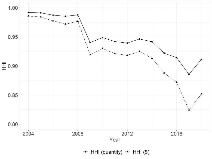
MILLENNIALS AND THE TAKE-OFF OF CRAFT BRANDS:
               PREFERENCE FORMATION IN THE U.S. BEER INDUSTRY

                                      Bart J. Bronnenberg
                                      Jean-Pierre H. Dubé
                                          Joonhwi Joo

                                          March 2021

We are extremely grateful to Ken Elzinga for sharing his U.S. beer industry database. We
benefited from the comments and suggestions from Matt Gentzkow, Elisabeth Honka, Mingyu
Joo, Xinyao Kong, Jin Miao, Olivia Natan, Ralph Siebert and from seminar participants at
Harvard, the 2020 ISMS Marketing Science conference, the Symposium on Consumer Analytics
and Data Science in Marketing and the 2021 Bass FORMS conference at UTD. We also thank
Andrew Wooders and Hwikook Choe for excellent research assistance. We are grateful to the
University of Chicago Kilts Center for Marketing for providing the Nielsen data. Authors own
analyses calculated (or derived) based in part on data from The Nielsen Company (US), LLC and
marketing databases provided through the Nielsen Datasets at the Kilts Center for Marketing Data
Center at The University of Chicago Booth School of Business. The conclusions drawn from the
Nielsen data are those of the authors and do not reflect the views of Nielsen. Nielsen is not
responsible for, had no role in, and was not involved in analyzing and preparing the results
reported herein. Dubé gratefully acknowledges the research support of the Charles E. Merrill
fellowship.

© 2021 by Bart J. Bronnenberg, Jean-Pierre H. Dubé, and Joonhwi Joo. All rights reserved. Short
sections of text, not to exceed two paragraphs, may be quoted without explicit permission
provided that full credit, including © notice, is given to the source.
Millennials and the Take-Off of Craft Brands: Preference Formation in the U.S. Beer Industry
Bart J. Bronnenberg, Jean-Pierre H. Dubé, and Joonhwi Joo
March 2021
JEL No. D12,L1,M31
ABSTRACT
We conduct an empirical case study of the U.S. beer industry to analyze the disruptive effects of
locally-manufactured, craft brands on market structure, an increasingly common phenomenon in
CPG industries typically attributed to the emerging generation of adult Millennial consumers. We
document a generational share gap: Millennials buy more craft beer than earlier generations. We
test between two competing mechanisms: (i) persistent generational differences in tastes and (ii)
differences in past experiences, or, consumption capital. Our test exploits a novel database
tracking the geographic differences in the diffusion of craft breweries across the U.S.. Using a
structural model of demand with endogenous consumption capital stock formation, we find that
heterogeneous consumption capital accounts for 85% of the generational share gap between
Millennials and Baby Boomers, with the remainder explained by intrinsic generational
differences in preferences. We predict the beer market structure will continue to fragment over
the next decade, over-turning a nearly century-old structure dominated by a small number of
national brands. The attribution of the share gap to consumption capital shaped through
availability on the supply side of the market highlights how barriers to entry, such as regulation
and high traditional marketing costs, sustained a concentrated market structure.
Bart J. Bronnenberg Joonhwi Joo
Tilburg University and CentER University of Texas at Dallas
Warandelaan 2, Koopmans K-1003 800 W. Campbell Rd.
5037 AB Tilburg JSOM 13-326
The Netherlands Richardson, TX 75080
bart.bronnenberg@uvt.nl joonhwi.joo@utdallas.edu
Jean-Pierre H. Dubé
University of Chicago
Booth School of Business
5807 South Woodlawn Avenue
Chicago, IL 60637
and NBER
jdube@chicagobooth.eduKeywords: branding, consumption capital, formation of preferences, market structure,
craft beer
JEL: D12, L11, M31, M37
1 Introduction
“The weakness in the received theory of choice, then, is the extent to which it relies
on differences in tastes to ‘explain’ behavior when it can neither explain how tastes are
formed nor predict their effects.”(Becker, 1976, p. 133)
Concentration and markups in the U.S. manufacturing sector have been rising for the past two
decades (e.g., Autor et al., 2017; Ganapati, 2018; Berry et al., 2019). However, the U.S. consumer
packaged goods (CPG) industry has emerged as an exception, with the dominance of large, es-
tablished national CPG brands over the past half century (e.g., Bronnenberg et al., 2007, 2009)
eroding in recent years with falling sales and market shares (eMarketer eMarketer Editors, 2019):
“In 2016, the top 20 consumer packaged goods companies saw flat sales, while smaller
firms averaged 2.9% growth. This follows four years, 2011 to 2015, in which large
CPG companies lost an estimated $18 billion in market share to craft manufactur-
ers.”(13D Research, 2017)
By 2018, 16,000 smaller CPG manufacturers accounted for 19% of all U.S. CPG sales, an increase
of 2 percentage points ($2 billion) over the previous year. That same year, the 16 largest CPG
manufacturers accounted for 31% of CPG sales, down from 33% five years earlier (eMarketer
eMarketer Editors, 2019). This rapid growth of smaller brands represents a striking, structural
break in the historically high and persistent concentration of CPG categories and the dominance
by large, national brands.
Industry experts routinely point to a demand-side explanation for this shift, identifying the
generation of Millennials – consumers born after 19801 – as the leading cause of this decline in
the sales of established brands:
1 Weuse the Pew Research Center definition at https://www.pewresearch.org/politics/2015/09/03/the-whys-and-
hows-of-generations-research/generations_2/ accessed on 12/2/2020.
2“They want to purchase brands that better align with their own values, whether it
be their dietary nutrition preferences, sustainability, philanthropy, etc.” (Howe, 2018;
Yue, 2019)
Surveys routinely find that Millennials seek smaller brands with more authentic products: “Nat-
ural, simpler, more local and if possible small, as small as you can.”(Daneshkhu, 2018) As a re-
sult, industry experts associate these declines with a generational share gap fueled by Millennials
with fundamentally different intrinsic preferences. A short-coming of this theory is the lack of a
mechanism for understanding why Millennials might form intrinsically different tastes from older
generations.
We propose an alternative consumption capital theory (Stigler and Becker, 1977) for these gen-
erational differences in CPG purchase behavior and the disproportionate preference for emerging
craft and artisanal goods amongst Millennials. Maintaining the neoclassical assumption of stable
tastes, we hypothesize that generational differences in behavior reflect heterogeneity in the accu-
mulation of consumption and brand capital (Bronnenberg et al., 2012). Older generations of con-
sumers had already accumulated decades of consumption capital with established, national brands
by the time that new craft and artisanal CPG products started to enter. In contrast, the younger
Millennial generation of consumers often had access to both craft- and established national brands
as they started to form their shopping habits.
We conduct an empirical case study of the take-home segment in the U.S. beer industry, one
of the leading examples of an industry disrupted by the sudden emergence of craft brands, which
grew from $10 billion to $29.3 billion between 2010 and 2019.2 Surveys indeed find a striking
generational share gap with half (50%) of older Millennials (25-34 year olds) drinking craft beer,
in contrast with 36% of U.S. consumers overall (e.g., Herz, 2016). As with other CPGs, Millen-
nials may value the perception of higher quality for craft beer: 43% of Millennial generation and
Generation X consumers (born between 1965 and 1980) state that craft beer tastes better than na-
tional brands, in contrast with only 32% of Baby Boomers (born between 1946 and 1964) (e.g.,
Mintel, 2013). Unlike earlier generations that only had access to large, established national beer
brands, Millennials have had access to a wide array of craft beers since their early adulthoods,
2 SeeStatista: https://www.statista.com/statistics/267737/retail-dollar-sales-of-craft-beer-in-the-us/ referenced on
12/2/2020.
3leading to different lifetime consumption experiences with nationally-branded and craft beer. The
recency of the availability of craft beers reflects, in part, deregulation, lower entry costs due to the
automation of the brewing process, the emergence of cheaper digital advertising formats and the
scalability of organic, online word-of-mouth marketing.
To test between the two theories – inherently heterogeneous generational preferences versus
heterogeneous consumption capital – we exploit the geographic differences in the timing and speed
of diffusion of new craft beer brewers and local availability of craft beer. We manually assembled
a novel database from various industry sources that tracks the history of all the craft beer brands
sold in the U.S. with a unique universal product code (UPC) in the take-home market. For each
UPC, we observe the product attributes, including beer style and alcohol content, the launch date
and location of the brewer, and the eligibility of each brewery for official “craft” designation going
back to the 1970s, when the first craft brewers entered the market. We match this beer census
with the Nielsen-Kilts Homescan database (HMS), containing the 2004-2018 purchase activity for
a nationally representative shopping panel of over 100,000 U.S. households. During the sample
period, the craft beer segment collectively increased from 5.3% in 2004 to 20% in 2018 based on
revenues, and from 5% to 12% based on volume. In 2018, Millennials accounted for 20% of total
craft beer sales and allocated 34% of their beer expenditures to craft brands, in contrast with 20%
for the much larger group of Baby Boomers.
The endogeneity of craft brewer entry into markets combined with the potential self-selection
of consumer types across markets complicates the determination of a causal effect of craft beer
availability. Our empirical strategy combines the panel structure of our data, to control for persis-
tent differences between markets, and two sets of instrumental variables that have been shown in
previous work to be drivers of brewer entry decisions: current and historic local population and
local time since the state-level legalization of brew pubs. Both instruments explain a substantial
portion of the variation in availability across markets and time. A series of suggestive placebo tests
support the hypothesized exogeneity of these instruments.
To disentangle persistent generational differences in tastes and consumption capital, we extend
the brand capital stock model of Bronnenberg et al. (2012). Reduced-form analysis of the model
reveals an important role for local availability in consumers’ craft versus nationally-branded beers.
After additionally controlling for historic availability when a consumer turned 21 and started to
4accumulate consumption capital, the persistent generational differences in tastes become small
and statistically insignificant even though we still detect heterogeneity along other socio-economic
dimensions.
The structural analysis of craft beer purchases confirms a dominant role for past experiences
to drive current purchase behavior through brand capital. We estimate a slow rate of depreciation
of consumption capital, indicating persistence in the effects of past experiences. In our full model,
we fail to detect significant differences in persistent preferences between, for instance, Millennials
and Baby Boomers. Even in a version of our structural model that restricts the availability effect
to be zero, generation effects alone account for at most 34% of the generational share gap at the
5% significance level. In spite of the lack of generational heterogeneity, our structural estimates
reveal heterogeneity in intrinsic preferences driven by other socio-economic traits than generation.
Education moderates craft beer demand, consistent with past research on product knowledge and
objective product quality (Bronnenberg et al., 2015). We also find a non-trivial income effect,
likely due to the price premium typically charged for craft brands.
To quantify the role of consumption capital in driving the observed generational share gap,
we conduct a series of counterfactual simulations with the model that equalize past craft brand
availability across generations. We find that 85.3% of the generational share gap is explained by
consumption capital. Therefore, Millennials buy craft beer at higher rates than older consumer
generations; but the differences in intrinsic preferences cannot account for the disruption to the
market structure of established beer brands. Instead, generational differences in craft beer demand
are mostly an artifact of generational differences in the historic availability of brands during early
adulthood.
To analyze the implications of consumption capital for the evolution of the market structure of
the U.S. beer category, we use our estimates to predict the cross-household average annual craft
beer share through 2030. Our estimates imply sustained growth in the craft beer share, reaching
almost 30% of the market by 2030. This growth primarily reflects the changing composition of
beer consumers as older generations die and a new generation of new adults – Generation Z –
enters the market and forms beer preferences.
Our findings add to the growing literature on consumption capital accumulation and the evolu-
tion of brand tastes (e.g., Bronnenberg et al., 2009, 2012; Sudhir and Tewari, 2015). These findings
5bolster the important role of past experiences in our understanding of heterogeneous preferences
across consumers, confirming the critical role of availability as a barrier to entry into consumer
goods markets.
Our findings also illustrate how consumer preferences can be shaped over time by the supply
side of the market, in this case through entry and availability. This finding suggests an important
role for the literature on industry dynamics (e.g., Ericson and Pakes, 1995; Pakes and Ericson,
1998; Doraszelski and Pakes, 2006) to incorporate the inter-dependence between supply and de-
mand on the formation of preferences and the impact on the long-term market structure.
Due to its size and history, the beer category has generated a literature unto itself (e.g., Adams,
2006; Garavaglia and Swinnen, 2017) with recent attention paid to the disruptive effects of craft
brands on the industrial market structure (e.g., Elzinga et al., 2015; Elzinga and McGlothlin, 2019).
We contribute to this literature by testing for and measuring consumption capital which introduces
a barrier to entry for new products. We also show that the dominance of established national brands
will likely continue to erode as more young consumers reach adulthood with access to a broader
variety of beer products from which to choose. However, a recent wave of craft brewer acquisitions
by the leading national brand manufacturers may reverse the trends in firm, as opposed to brand,
concentration.
The remainder of the paper is structured as follows. We provide a brief summary of the evolu-
tion of the U.S. beer market structure and the impact of craft brewing in section 2. We describe the
data in section 3. Section 4 documents the generational share gap and section 5 develops a model
of consumer demand with consumption capital formation. We present our empirical strategy and
results in section 6, and our counterfactual analysis of availability and its effect on the generational
share gap and market structure in section 7. We conclude in section 8.
2 The Craft Beer Market
A detailed history of the beer market structure and the evolution of the craft movement is beyond
the scope of this paper. We refer the interested reader to Adams (2006) for a detailed account of
the U.S. beer market, to Garavaglia and Swinnen (2018) for the economic impact of the craft beer
movement, and to Hindy (2014) for an industry insider’s account.
6Prior to the emergence of craft brewers, the beer industry was highly concentrated by the 1970s,
dominated by Anheuser-Busch, Miller, Schlitz and a small group of other macrobreweries. Tech-
nological innovation in brewing and packaging coupled with mass advertising, especially on tele-
vision, established high barriers to entry (Adams, 2006; Noel, 2009; Garavaglia and Swinnen,
2018). To generate scale economies, U.S. brewers mostly supplied lager beers3 described by ex-
pert Michael Jackson as “lacking hop character and generally bland in palate,” (Alworth, 2015, p.
29) making “the beer landscape blander and more boring.” 99% of beer consumed in the U.S. was
pale lager beer (Elzinga et al., 2015).
The timing of the start of craft brewing coincided with the elimination of a legal barrier to
entry.4 In February 1979 (e.g., Elzinga et al., 2015), President Carter repealed prohibition-era
restrictions on home brewing, with H.R. 1337 legalizing home brewing federally and allowing
states to begin implementing their own laws. This repeal was not in response to changing beer
demand, but rather part of Carter’s broader agenda to deregulate and “reduce excessive government
intrusion into the private affairs of American citizens.”5 While many craft brewers started off as
home brewers, it was not until 1982 that Washington became the first state to legalize commercial
brewpubs, triggering a series of state-level laws across the U.S. that legalized commercial sale of
craft beer and modified the corresponding licensing fees and taxes. By 1990, over half the states
had legalized brewpubs, and by 1999, all states had legalized brewpubs (Elzinga et al., 2015).
The take-off of the craft beer market share was initially slow due to poor pricing practices,
high costs and a quasi-monopoly over distribution by the incumbent macrobreweries that led to
waves of shakeouts in the 1980s and 1990s (e.g., Hindy, 2014; Noel, 2018). With the exception
of the Boston Beer Company, few craft brewers had the financial resources to rely on traditional
media – television and radio advertising – to generate awareness and build brands. The legaliza-
tion of brewpubs “provided perhaps millions of Americans with their first encounters with craft
beer.” (Acitelli, 2017, p.217) The rise of the internet in the early 1990s is widely believed to have
catalyzed growth in the craft market share: “The internet has arguably been the greatest ally of
3 Scale economies are even more pronounced for lager beers that incur higher fixed costs from the need for more
artificial cooling and longer fermentation times than other beer styles, like ales (Garavaglia and Swinnen, 2018).
4 The brewing trade press times the debut of the U.S. craft beer movement to 1965, when Fritz Maytag took over
the Anchor Steam Beer Company and focused operations on traditional beer flavors produced in small scale and
emphasizing its local “made in San Francisco since 1896” image (Acitelli, 2017).
5 This statement comes from Carter’s debate with Reagan on October 28, 1980. Accessed on 8/22/2020 at
https://www.debates.org/voter-education/debate-transcripts/october-28-1980-debate-transcript/.
7the craft beer revolution. [...] Today nearly every craft brewer has a website and someone to talk
directly to its customers and fans through social media.” (Hindy, 2014, p.144). The disruptive
force of the internet is not exclusive to the beer industry. It has also disrupted numerous CPG cat-
egories by facilitating successful start-ups like Dollar Shave Club, for razors, and Barkbox, for pet
supplies.6 In addition, “Associations of craft consumers, craft brewers, and homebrewers helped
expand the market by spreading information and experiences, and being a vehicle for new forms
of marketing (often via the internet, social media, and special events).”(Garavaglia and Swinnen,
2017, p. 43). The merger of the Association of Brewers and the Brewers’ Association of America
in January of 2005 allowed small brewers to organize to compete more effectively (Hindy, 2014),
leading to a take-off in the segment that reached 3,490 U.S. craft breweries by 2015, in contrast
with only 249 in 1990.
In addition to the erosion of barriers to entry, demand-side factors also likely contributed to
the recent take-off in craft beers supplied to the market. Rising incomes enabled beer consumers
to pay the price premium associated with a craft product supplied at a higher marginal production
costs. Consumers may also genuinely perceive a superior-quality taste from beers brewed using
traditional, small-scale methods. Alternatively, consumers may value the authenticity of a local,
small-scale product. Macro brewers also attempted to counteract craft brewers by launching their
own traditional-beer-style brands such as Blue Moon, by Coors, and Budweiser American Ale,
by Anheuser-Busch. Thus far, such corporate launches have not been successful at dominating
craft brewers outside the pale lager style category. However, the recent wave of acquisitions of
successful craft brewers by Anheuser-Busch, Miller-Coors and other large macrobreweries does
not appear to have decreased demand for those brands even after losing their craft status (Elzinga
and McGlothlin, 2019). None of these demand-side factors suggest why Millennials per se would
be the drivers of craft beer market share growth.
Since craft brewers represented mostly a fringe of the U.S. beer market until the early 2000s,
most generations of consumers reached the legal drinking age of 21 facing a choice set comprising
primarily large macrobreweries selling established brands of pale lager beers. Only the youngest
6 According to the 2019 Online Consumer Packaged Goods Report, 34 CPG companies appeared in the top-1000
internet retailers, 19 of which sell and manufacture consumer brands. Just like the recent wave of acquisitions of craft
brewers by Anheuser-Busch, many established CPG conglomerates in other product categories have begun acquiring
digital start-ups such as Unilever’s $1billion acquisition of Dollar Shave Club and Campbell Soup’s recent $10million
investment in Chef’d.
8Generation X and Millennial consumers had access to craft brands on the shelves at the moment
they reached the legal age to drink. Our focus herein is to test for such a timing effect on demand
and to measure its relative magnitude compared to persistent generational differences and other
socio-economic drivers of demand.
3 Data
3.1 Beer Characteristics
We manually assemble a census of bar coded, non-draught beers available in the U.S. using the
digital repositories at three industry associations: the Brewers’ Association (BA), the American
Breweriana Association (ABA), and the website ratebeer.com. For each Universal Product Code
(UPC), we observe the corresponding brewer, style (e.g., ale, lager, stout, etc.), alcohol by volume
(ABV), quality ratings (on a 1-5 scale) and, most importantly, craft status. In total, we observe
36,214 unique UPCs.
We classify a brewer, and by association each of its UPCs, as craft if it meets either of the
following criteria: (i) ratebeer.com classifies the brewer as a “Microbrewery”, “Brew Pub” or
“Brew Pub/Brewery” in 2018; or (ii) the BA has classified the brewer as “independent craft brewer”
in 2018. We assume that any brand that is classified as craft in 2018 has always been a craft beer
since its launch.7 This classification includes many well-known craft brewers, including those that
have expanded across states and to the national level, like Yuengling or the Boston Beer Company
(widely known for its Sam Adams brand). In total, 63% of the UPCs (22,130) satisfy our craft
definition.
While our craft classification scheme reflects the criteria of the leading beer association, the
BA, it nevertheless excludes a few former craft brewers, such as Goose Island in Chicago, that were
acquired by macro brewers like Anheuser-Busch during the sample period, even though consumers
may continue to perceive their brands as craft. This exclusion affects the craft share in 2018 by
only 0.6%.
We classify all other UPCs in our data as national brands produced by macro brewers. While
7 Neither the BA nor ratebeer.com reports historic time-series data on past, annual craft designations.
9this set includes many, often small, foreign brewers, macro brewer volume is highly concentrated
amongst the largest brewers such as Anheuser-Busch, Heineken, and Miller-Coors.8
As expected, national brands are differentiated from craft brands along several dimensions.
We observe a quality rating for 92% of the UPCs. On average, national brands are lower quality
than craft beers with average ratebeer.com ratings of 2.4 and 3.3 (out of 5), respectively. National
brands also tend to have a lower alcohol content, with an average ABV of 5.3% compared to 6.5%
for craft beers. Some of these quality differences may reflect differences in beer styles. National
brands are most likely to be lager style, whereas craft brands are most likely to be Indian Pale Ale
(IPA), Pale Ale, or Amber Ale. For instance, the average quality rating of a national brand is 2.1
out of 5 in the lager category and 3.3 in the IPA category. But, even after residualizing on beer
style and alcohol content, national brands are still significantly lower quality than craft beers with
average ratings of 2.35 and 2.84, respectively (F-stat 7,570). This quality difference is consistent
with the standard perception that craft beers have better flavor due to their production methods and
ingredients. Therefore, for the remainder of the analysis, we focus on the differences in demand
for craft versus national brand beers rather than focusing more granularly on demand for specific
beer styles.
3.2 Household Panel Data
We use the Nielsen Homescan Panel (HMS) of U.S. households between 2004 and 2018 to mea-
sure households’ beer purchases in the take-home market. The take-home market consists of pre-
packaged, bar-coded beer products sold for home consumption in retail outlets such as supermar-
kets, mass merchants, convenience stores, drug stores and liquor stores. The database contains
186,233 unique households during the sample period, with an average of about 39,000 households
per year from 2004-2006 and 61,000 households per year from 2007-2018. For each household, we
observe the date of each trip to a store selling beer along with the specific products purchased, as
designated by their unique UPC, and the corresponding quantities and prices paid net of discounts.
For each year, we retain those households that purchase beer at least once using the Nielsen prod-
uct modules “Beer,” “Near Beer,” “Stout and Porter,” “Light Beer,” and “Ale” (i.e., module codes
8 Usingour Nielsen HMS data from 2004-2018, the top 10 macro brewers combined represent 88% of total beer
volume purchased by our HMS panelists and 95% of macro brewer volume.
105000, 5001, 5005, 5010, and 5015, respectively). Our HMS data contain beer purchases from
104,115 unique households.
We match the HMS data with Nielsen’s annual demographic survey of panelists to determine
a household’s income and size (# members). We also use the age (in years) and education attain-
ment of the head of household, defined as the oldest head of household reported in the Nielsen
demographic survey. Education attainment takes on one of six categorical values: Grade School,
Some High School, High School Diploma, Some College, 4-year College degree, and Post College
Degree. For household income, we use the mid-point of each of the 16 income brackets reported
in the survey, top-coding the “above $100,000” category at $150,000.
We classify each household into a generation based on the year of birth of the oldest current
head of household. We use the Pew Research Center’s generation definitions as follows9 :
• Millennial Generation: born between 1981 and 1996
• Generation X (hereafter GenX): born between 1965 and 1980
• Baby Boom Generation (hereafter BB): born between 1946 and 1964
• Silent Generation (hereafter SG): born between 1928 and 1945
• Greatest Generation (hereafter GG): born before 1928.
Since our sample period ends in 2018, we have a very small number of adults born after 1996 who
are technically part of Generation Z (born after 1996). For our empirical analysis, we combine
these households with the Millennials.
Each HMS household is assigned to a Nielsen Scantrack based on its geographic location.
Most Scantracks represent a large metropolitan area (e.g., San Diego) or a part of a state (e.g., West
Texas). However, 20% of beer buying HMS households live in rural areas that are not covered by
a Scantrack definition and, hence, are classified as “Remaining U.S..” We cannot assign historic
information regarding craft brand availability to these households, and therefore these households
are discarded from our analysis. This leaves us with 83,187 households, which we use as our final
sample.
9 https://www.pewresearch.org/fact-tank/2019/01/17/where-Millennials-end-and-generation-z-begins/ accessed on
12/15/2020
11We match the remaining HMS households’ beer purchases with the beer characteristics database
using UPCs and brand names. We successfully match over 95% of the UPCs purchased by our
HMS panelists, accounting for 97% of the total beer volume purchased during the sample period.
HMS panelists purchase 20,816 unique beer UPCs, or 57% of all UPCs available in our beer char-
acteristics file. Recall that our original beer attribute file tracks an approximate census of all beer
sold in the U.S. take-home market during the sample period, whereas the HMS sample only tracks
those beers purchased by the panelists.
Our final HMS beer sample consists of 2.6 million unique beer transactions from 83,187 unique
households. Table 1 describes the sample. The average household remains in our sample for 4
years, with the 5th and 95th percentile tenure of 1 year and 13 years, respectively. On average,
a household conducts 6.8 transactions per year; with the 5th and 95th percentile frequency of 0.7
and 29.0, respectively. The average household purchases 166.9 ounces of beer per trip (slightly
more than a 12-pack of 12-oz bottles or cans). Of all sizes, 12-pack cases constitute the most
frequently-chosen pack size, accounting for 25.2% of all transactions. Finally, households spend
an average of $11.94 per trip, with the 5th and 95th percentile expenditure levels of $4.28 and
$22.38, respectively.
For the analysis below, we collapse the HMS transaction panel to 270,347 household-year
observations. For each household, we compute the annual craft share of beer volume purchased.
Table 1 describes the sample. While the average annual household craft purchase share is 14.2%,
we observe a large degree of heterogeneity with 10th and 90th percentile shares of 0% and 67%,
respectively.
We also observe a diverse set of households in the sample. Across households and years, the
average age of household heads in our purchase data is 54 years with 90% of the household-years
between 32 and 78. The average number of years of education is 15, with 90% of the households
between 12 and 18 years. The average annual household income is $65K, with 90% between
$17.5K and $120K. Finally, the average household size is 2.6 members, with 90% of households
having between 1 and 5 members.
Finally, across households and years, 4% of our observations are Millennials, 18% GenX, 52%
BB, 23% SG and 3% GG. The share of Millennials in our sample grows from 0.1% in 2004 to
11.2% in 2018 (or to 19.6% in 2018 if we use Nielsen’s projection factors to re-weight households
12for national representativeness). Even though Millennials are the youngest panelists in our sample,
they have completed more years of education than older generations and have comparable incomes.
For instance, the average Millennial has 16 years of education in 2018 and earns an average income
of $73K. In comparison, the average years of education and average income in 2018 is 15 and
$74K, respectively, for BBs and 16 and $81K, respectively, for GenXs.
—– include Table 1 here —–
3.3 A Measure of Local Craft Beer Availability
Even though our HMS purchase data reflect retail beer sales, we expect consumer awareness for
craft beer to be influenced by local craft entrepreneurship more broadly, including brew pubs and
other craft beer establishments with on-premise sales. We use the BA, ABA, and ratebeer.com
digital archives to assemble an annual census of U.S. brewers by market from 1979 to 2018.
To determine the number of local craft brewers, we use the ABA’s census of U.S. brewers,
which contains each brewery’s geographic location along with its opening and, when applicable,
closing date. We match the brewer census with the ratebeer.com and the BA databases, retaining
only those brewers satisfying the craft criteria defined in section 3.1 above. Since many of the
brewers in this broader sample do not sell beer with a unique UPC, we use a fuzzy matching
scheme to determine their craft status. See Appendix A for details regarding the matching criteria.
To verify that our craft census did not admit any macro brewers, we processed the remaining
brewer names against a pre-determined list of substrings like “Anheuser,” “Miller,” and “Molson”
from the largest non-craft brewers representing 99% of the non-craft beer volume in our HMS
sample. After removing all additional matches, we classify all the remaining brewers as craft.
We normalize the craft beer availability in each market using the annual census of U.S. macro
brewers compiled in the Elzinga-Tremblay-Tremblay database (Elzinga et al., 2015) spanning the
period from 1979 to 2012. While the census ends in 2012, the total number of macro brewers
was quite small and stable with 19 brewers between 2007 and 2012. Therefore, we assume the
number of macro brewers remained stable at 19 through 2018. Finally, we assume macro brewers’
products were available in all markets.
C denote the number of craft brewers in market m during year
To measure availability, let Nmt
13t. As explained in section 2, craft brewers first emerged in 1979 with the legalization of home
C = 0 ∀t < 1979. Since we assume that macro brewers are available in all
brewing. Therefore, Nmt
markets, we let NtNB denote the count of macro brewers in year t. We use the local share of craft
C
Nmt
brewers in each market m and year t as our availability index: Dmt = Nmt +NtNB
C .
C , during our sample period.
We observe rapid growth in the number of local craft brewers, Nmt
The cross-Scantrack average grew from 20 in 2004 to 67 in 2018. In 2004, the cross-Scantrack
C were 2 (Birmingham, AL), 79 (Portland, OR)
minimum, maximum, and standard deviation of Nmt
and 18. For 2018, these numbers were 6 (Memphis, TN), 300 (Denver, CO), and 61.
The whisker plot in Figure 1 displays the corresponding two-year, cross-Scantrack distribution
of our availability index, Dmt , between 1978 and 2018. Two patterns emerge. First, we observe
substantial cross-market heterogeneity in the availability of craft brewers and the rate of growth.
Not only do we observe growth in the median availability, we also observe growth in the inter-
quartile range across markets. Second, we observe two national, industry-wide waves of craft
brewer entry, first in the early 1990s and later in the 2010s. Interestingly, the lower bound of the
centered 90% quantile interval grows most rapidly in the final years of the sample as the laggard
markets catch up with their craft beer availability.
—– include Figure 1 here —–
This heterogeneous evolution in availability across markets generates useful variation in the
extent of craft beer available when our panelists turned 21 and were legally able to buy beer. Figure
2 displays the distribution of Dmt at 21 years old by generation. Since the craft beer movement did
not start until 1979, Dmt is mechanically zero for our two oldest generations: Greatest Generation
and Silent Generation. Even for the Baby Boomers (the youngest of whom turned 21 in 1985), the
average availability is quite low, less than 0.1, due to the fact that the average number of local craft
brewers for this generation in the year they turned 21 is 1. For GenX, the average is approximately
0.18. But, for Millennials, the average availability of local craft brewers in the year they turned 21
is almost 0.4, more than double the availability for GenX.
—– include Figure 2 here —–
143.4 Population Data
To determine each Scantrack’s population from 1969 through to 2018, we use the regional popula-
tion data provided by the National Cancer Institute’s Surveillance, Epidemiology, and End Results
(SEER) Program.10 The SEER data track annual, county-level population. We then use Nielsen’s
mapping between FIPS codes and Scantracks to determine the Scantrack populations.
3.5 State-Level Brewpub Laws
We use Elzinga et al. (2015, Table 2) to determine the exact year each U.S. state legalized commer-
cial brewpubs, enabling local home brewers to sell their beer at a small scale while by-passing the
three-tier distribution system required for larger brewers. Even though homebrewing was federally
legalized in 1978, only in 1982 did Washington become the first state to legalize brewpubs, and it
was not until 1999 that Mississippi and Montana became the last two states to legalize brewpubs.
Due to the nature of diffusion, we expect the number of years since state legalization to be predic-
tive of the diffusion of brewpubs and, accordingly, to predict some of the cross-state differences in
craft beer availability.
3.6 Census Data
To determine the rate at which new Millennial and Generation-Z consumers reach adulthood and
enter the beer market after the sample period, we use the Census projections for 2019-2030.11 For
each year, these projections include total U.S. population with a breakdown by age. We also use
these projections to determine the mortality rates for our older generations of beer consumers.
4 Craft Beer and the Generational Share Gap
We begin by using the HMS sample to document the generational differences in craft beer purchase
behavior. Due to their smaller production scale and emphasis on higher-quality ingredients, craft
and artisanal consumer products tend to be more expensive. Therefore, we also anticipate that
10 https://seer.cancer.gov/popdata/ accessed on 8/16/2020.
11 https://www2.census.gov/programs-surveys/popproj/datasets/2017/2017-popproj/np2017_d1_mid.csv accessed
on 12/10/2020
15demand for craft products will depend, in part, on socioeconomic status (SES). Since SES likely
correlates with generations, we control for SES in our analyses. In particular, we use household
income, household size, and household education to control for SES and factors correlated with
SES.
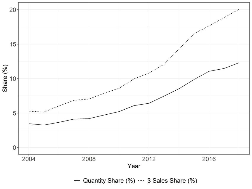
Craft beer has disrupted the long-established dominance of macro brewers and their established
brands. The left panel of Figure 3 plots the annual national craft share both in volume and dollars.
The craft share of volume grew from approximately 5%, in 2004, to approximately 12%, in 2018.
The revenue share grew even faster, largely due to the craft price premium, reaching nearly 20%
of beer sales in 2018. The 2018 HMS craft volume and revenue shares are close to the 13.2% and
24.1% reported by the BA for the entire U.S. market.12 Even amongst the largest macro brewers,
overall revenues have increasingly fragmented over time as acquired craft brewers represent an
increasing portion of their sales. In Figure 4, we show that AB-InBev’s HHI across its owned
breweries has decreased from 0.986 in 2004 to 0.852 in 2018. This decline largely reflects the
declining share of AB-InBev revenues coming from its two top brands, Budweiser and Bud Light,
for which the share fell from 49.1% in 2004 to 40.9% in 2018. By 2018, 33% of the craft beer
volume sold was supplied by brewers that had been acquired by a macro brewer. In sum, the recent
growth in craft beer has fragmented both the category as well as some of the largest firms’ revenue
sources.
—– include Figure 3 here —–
—– include Figure 4 here —–
During this same period, we also observe rapid growth in the number craft UPCs purchased
by HMS panelists. The total annual count increased from 1,008 (32% of all UPCs purchased by
panelists), in 2004, to 4,961 (67% of all UPCs purchased by panelists), in 2018. In contrast, the
total number of macro brew UPCs purchased by HMS panelists remained quite stable with 2,185
in 2004 and 2,460 in 2018. These findings are consistent with the escalation in craft brewer entry
and stable macro brewer presence during our sample period, as described in section 3.3. These
patterns are suggestive of a role for availability and variety in the growth of the craft beer segment.
12 https://www.brewersassociation.org/press-releases/brewers-association-releases-annual-growth-
report/#:~:text=In%202018%2C%20small%20and%20independent,7%20percent%20growth%20over%202017
accessed on 9/8/2020.
16Our main interest is in the role of Millennial consumers in driving the growth of craft beer. The
right panel of Figure 3 displays the evolution of each generation’s share of craft beer purchased.
Due to their young age, Millennials represented less than 1% of craft volume in 2004. By 2018,
Millennials accounted for almost 20% of craft volume sold in spite of the much larger number
of Baby Boomer households in the U.S.. With the exception of Millennials, every other genera-
tion’s share of craft volume sold decreased between 2004 and 2018. Therefore, even though all
generations are purchasing craft beer, Millennials are driving most of the growth.
Figure 5 displays our key stylized fact: the generational share gap. The bars indicate each
generation’s mean annual craft share of beer volume sold across households and years. The dia-
monds indicate the analogous mean craft share for each generation, residual of our SES controls.
Households belonging to the Greatest Generation have a low craft beer share at 6%. In contrast,
Millennials have a 19% share, 11.5 percentage points higher than Baby Boomers and 7 percentage
points higher than GenXers. These pooled differences may confound the changing composition
of household generations through our sample period. Focusing on 2018, our most recent sample
year, the generational share gap is even larger with Millennials purchasing 34% craft beer versus
13% for the Greatest Generation and 20% for Baby Boomers. This share gap is robust to SES
controls, even though each generation’s mean annual share decreases after residualizing on SES.
The remainder of the paper seeks to explain the 12 percentage-point generational share gap be-
tween Millennials and Baby Boomers. In the next section, we test and quantify the relative roles
of intrinsic generational differences in preferences and generational differences in historic brand
experiences that generate the accumulation of consumption capital for craft beer brands.
—– include Figure 5 here —–
5 A Consumption Capital Stock Model of Demand
To quantify the extent to which differences in craft beer purchases across generations reflects in-
trinsically different preferences versus consumption capital accumulation, we use the consumption
capital stock model from Bronnenberg et al. (2012). Unlike the rational addiction literature which
treats consumption capital as a habit (e.g., Becker and Murphy, 1988), we think of consumption
capital herein as the component of a consumer’s preference for craft beer due to past consumption
17experiences. The model allows us to disentangle the extent to which a consumer’s craft purchase
behavior is driven by persistently different preferences versus different historic consumption expe-
riences and availability.
We model each consumer’s choices between craft brands (CB) and national brands (NB). On
a given purchase occasion, a consumer derives the following incremental utility from choosing a
craft beer instead of a national brand:
∆U = α µ (D, X, ξ ) + (1 − α) k − ν
where µ (D, X, ξ ) represents the consumer’s baseline utility, which depends on the observed avail-
ability of craft brands, D, on the consumer’s generation and SES, X, and on other unobserved
consumer-specific factors of that year, ξ . µ (D, X, ξ ) captures the treatment effect of the con-
temporaneous choice environment. The variable k ∈ (0, 1) denotes the consumer’s consumption
capital stock at the start of the year and α ∈ (0, 1] determines the relative importance of accumu-
lated consumption capital on current choices. Finally, v ∼ Uniform (0, 1) is an i.i.d. random utility
shock drawn at each purchase occasion.
If the consumer makes beer brand purchases to maximize her conditional indirect utility then
she chooses CB if ∆U ≥ 0. The corresponding expected CB share of beer purchases is
y = α µ (D, X, ξ ) + (1 − α) k, (1)
which is the linear probability model of demand (e.g., Heckman and Snyder, 1997).
The consumer’s stock of consumption capital evolves as a discounted average of her past con-
sumption:
∑A−1
a=21 δ
A−a y
a
kA = A−1 A−a
(2)
∑a=21 δ
where A ≥ 22 is the consumer’s current age and ya is the consumer’s CB purchase share at age a. To
initialize consumption capital, we assume k21 = µ (D21 , X, ξ21 ). The degree of persistence in past
consumption on current beer choices is determined by the parameter δ ≥ 0. Therefore, evolution
in the availability of craft brands not only changes a consumer’s contemporaneous choices through
18(1), it also influences her subsequent consumption capital accumulation through (2).
To see the connection between this model and the traditional human capital stock accumula-
tion models (e.g., Becker, 1967), we can re-write the consumption capital stock (2) recursively as
follows:
kA = kA−1 (1 − ρA ) + yA−1 ρA (3)
where
1−δ
ρA = . (4)
1 − δ A−21
See Appendix B.1 for the proof. Conceptually, the net contribution to consumption capital at
the end of each period, kA − kA−1 , depends on the gross investment, ρA yA−1 , and depreciation,
ρA ∈ [0, 1]. At age 22, ρ22 = 1 and a consumer only responds to current availability and marketing,
µ (D22 , X, ξ22 ). In contrast, as a consumer ages, her consumption capital becomes less sensitive
to recent choices and the recent choice environment. The persistence parameter, δ , governs the
relative role of current versus past experiences on consumption capital. Note that lim ρA = 1,
δ →0
1
lim ρA = A−21 , and lim ρA = 0. Consequently, when δ < 1, consumption capital is affected more
δ →1 δ →∞
by consumers’ most recent experiences, and when δ > 1, consumption capital is affected more
by their earliest experiences during adulthood than recent experiences. Unlike the literatures on
investment in education and health capital (e.g., Grossman, 2000), we assume consumers are my-
opic about their consumption capital (i.e., consumers do not plan ahead for future years’ craft beer
consumption and associated consumption capital accumulation).
To derive our empirical formulation, we can re-write expected demand at age A ≥ 21 as a
weighted sum of the consumer’s experiences with past choice environment:
A
yA = ∑ ωA,a µ (Da , X, ξa ) (5)
a=21
where
A
∑ ωA,a = 1, ωA,a ≥ 0 ∀A, a.
a=21
See Appendix C for the proof. Therefore, demand is a distributed lag over a consumer’s entire
history of access to craft beer brands during her adult life (i.e., since 21). At the heart of our
empirical test for whether differences in craft purchase propensities reflect intrinsic differences in
19preferences versus differences in past brand experiences is the relative importance of differences
between consumer generations in µ (Da , X, ξa ) versus {Da }Aa=21 .
For our empirical implementation of the consumption capital model above, we re-cast the
model in calendar time. We define the contemporaneous choice environment in year t for a con-
sumer h living in market m (h) as follows:
µ Dm(h)t , Xh , ξht = φ (Xh ; Λ) I{D } + γDm(h)t + ξht (6)
m(h)t >0
where
φ (Xh ; Λ) = β0 + ∑ I{genh=g}βggen + ∑ I{educh=e}βeeduc +
g∈G e∈E
inc size
β Incomeh + β HouseholdSizeh + ∑ I{mktht =m} λ mkt
m∈M
represents a consumer’s time-invariant taste for craft beer and Λ = (β 0 , λ 0 ) is the vector of intrinsic
preference parameters, and Xh contains a household’s generation and SES variables. G , E and M
are the sets of observed generations, education levels, and Scantrack markets, and I{·} is the indi-
cator function. The interaction with the indicator I{D } ensures that expected craft demand is
m(h)t >0
only positive when craft beer is available. ξht is a mean-zero, unobserved (to the econometrician)
contemporaneous demand shock.
Using (5), we can therefore write consumer h’s craft beer share in year t as a distributed lag
over her adult life experiences with craft beer:
t
ωAht ,Ahτ (δ , α) γDm(h),τ + ξ˜ht
yht = φ (Xh ; Λ) ϖht (δ , α) + ∑ (7)
τ=t−Aht +21
where the weights ωAht ,Ahτ (δ , α) depend on the consumer’s age in the current year t and past year τ
respectively, as well as the non-linear parameters (δ , α), and ϖht (δ , α) = ∑tτ=t−Aht +21 ωAht ,ahτ (δ , α) I{D }
m(h)τ >0
is the sum of the weights over those adult years during which craft beer was available. Thus,
for a consumer that has always had craft beer available during her adult years (e.g., younger
Millennials), ϖht (δ , α) = 1. ξ˜ht = ∑tτ=t−Aht +21 ωAht ,ahτ (δ , α) ξhτ is the composite error term, a
weighted average of historic demand shocks and therefore E ξ˜ht = 0 and var ξ˜ht < ∞ since
20∑tτ=t−Aht +21 ωAht ,ahτ (δ , α) = 1 and Aht (≥ 21) is finite.
6 Structural Analysis of Demand
6.1 Endogeneity of Availability
There is good reason to expect craft beer availability to be exogenous to individual consumer
demand. As recently as 2009, Charlie Papazian, founder and president of the BA, explained: “I’d
say over 90 percent of small brewers I talk to today have roots in home brewing,”(Beato, 2009)
such that most craft brewers did not originate with the intention to generate profits per se. Since our
analysis controls for persistent between-market differences, the endogeneity would need to arise
from differential cross-market trends in unobserved demand. We envision two potential sources
of endogeneity bias. First, to the extent that craft brewers endogenously time their entry into a
market based, in part, on unobserved aspects (to the researcher) of demand, ξ˜ht , this simultaneity
could bias NLLS estimation of equation (7). In addition, there is potential measurement error in
our availability variable.
One potential source of measurement error arises if local brewers serves as an imperfect proxy
for perceived availability. Since the direction of the simultaneity bias from endogenous availability
is difficult to determine without a full-blown model of entry, it is difficult a priori to determine
the net effect of measurement error and simultaneity on a NLLS estimator that treats availability
as exogenous. A potential source of measurement error in historical availability rates arises from
households moving between markets prior to the sample period. We conduct two robustness checks
to rule out a bias due to unobserved moves. First, for the 3, 521 moves that are observed during
the sample period we observe the correct availability history and, although not reported herein, our
findings do not change if we assume these households always lived in their most recent market. In a
separate analysis, we used only those HMS panelists who responded to Bronnenberg et al. (2012)’s
Panelviews migration survey, allowing us to determine the correct availability history prior to the
sample period. Appendix Table 2 reports almost identical OLS estimates of the current and lagged
availability effects in reduced-form versions of (7) that correct versus do not correct for moves
prior to the sample period.
21To instrument for availability, we turn to the industrial organization literature on entry and mar-
ket structure in the U.S. beer industry to determine the exogenous influences on the local entry of
craft brewers into a market. A full-fledged analysis of the industry dynamics of entry and exit in
the U.S. beer market is beyond the scope of this paper.13 However, the recent empirical literature
studying the endogenous formation of the industrial market structure has routinely found popu-
lation, a proxy for potential market size, to be a critical determinant of market structure (Sutton,
1991; Bresnahan and Reiss, 1991), including in the U.S. beer industry specifically where popu-
lation predicts the historic number of local competing brewers (Manuszak, 2002; Elzinga et al.,
2015). We use each Scantrack market’s annual population as our proxy for market size. We also
use the number of years elapsed since each U.S. state legalized commercial brewpubs, allowing
for differential timing of diffusion across states. Although not reported herein, we also collected
a detailed database tracking changes in state and federal craft brewing laws related to permits and
fees; but these instruments had no power in explaining availability variation.
Figure 6 visualizes the correlation between the population instrument and the differential rate
of diffusion in craft beer availability across geographic markets and time. Each panel corresponds
to a year, t ∈ {1980, 1985, 1990, 1995, 2000, 2005, 2010, 2015} . Within each panel, we plot a circle
for each of our 53 Scantrack markets, with diameter proportional to that year’s availability, Dmt .
We also use shading of each circle to represent that year’s population.
—– include Figure 6 here —–
To quantify the power of the two instruments, we analyze the first stage of a linear version of
an IV estimator that includes current availability along with generation, SES and market-specific
effects and clusters standard errors on Scantrack-year combinations. We obtain an incremental
F-statistic for contemporaneous population of 468.83.14 Adding every 5th lag in population as
far back as 35 years prior to the current year generates a joint incremental F-statistic (current and
lagged population) of 110.14. Adding years since the state legalized brewpubs further increases
the power of the incremental F-statistic to 312.9. Persistent Scantrack differences explain 65% of
13 A related literature has also studied the role of recent large-scale mergers, acquisitions and joint ventures on the
industrial market structure of beer (e.g., Tremblay et al., 2005; Ashenfelter et al., 2015; Miller and Weinberg, 2017;
Elzinga and McGlothlin, 2019).
14 If we instead pool all 2,120 unique Scantrack-years from 1979 (start of craft brewing) to 2018 and regress avail-
ability on contemporaneous population, we obtain an incremental F-statistic of 2,255.11.
22the variation in availability, Dmt . Adding our excluded population instruments explains 80% of
the variation in Dmt and adding years since the state legalization of brewpubs explains 89%. In all
these specifications, the effect of both current population and years since the state legalization of
brewpubs are positive and statistically significant.
Formally, our key identifying assumption is that in any year s,
E ξhs qm(h,s)s = 0
where qm(h,s)s is the population in year s and the market, m (h, s), where household h lived in year
s. We have an analogous moment for the number of years since the state legalized brewpubs. We
cannot formally test these assumption. However, even after residualizing on market fixed effects,
the scantrack population is uncorrelated with the prevalence of beer drinkers (i.e., share of HMS
panelists with positive beer expenditures in a market-year) and also uncorrelated with the preva-
lence of Craft beer drinkers (i.e., the share of HMS panelists with positive expenditures on craft
beer in a market-year), generating correlations of –0.020 (0.035) and 0.038 (0.034), respectively,
where standard errors are in parentheses.15 Therefore, areas with higher population growth are not
systematically attracting more beer drinkers or more craft beer drinkers, factors that could indicate
strong local beer-drinking trends.
We also conduct two placebo tests. First, we test whether markets and years where contempo-
raneous local panelist SES variables predict high craft share also tend to have higher populations.
We predict household-year craft shares using market fixed effects and SES variables. We use
these estimates to predict the Scantrack-year level expected share. We find that population and
years since the state legalization of brewpubs are both negatively associated with this predicted
Scantrack-year share, so that if anything, population and the elapsed time since legalization both
tend to be smaller in markets with higher craft brand shares.
We also test whether markets and years where contemporaneous craft beer availability is high
also tend to have higher populations or tend to be markets that were earliest to legalize brewpubs.
In this case, we predict Scantrack-year availability using SES variables and Scantrack fixed-effects.
Once again, we find negative associations between predicted availability and population and years
15 We use the Nielsen projection factors to ensure our Scantrack panelists are representative of the actual population
23You can also read