MISSING GLOW PHENOMENON: LEARNING DISEN-TANGLED REPRESENTATION OF MISSING DATA
←
→
Page content transcription
If your browser does not render page correctly, please read the page content below
Submitted to the ICLR 2021 Workshop on Geometrical and Topological Representation Learning
M ISSING G LOW P HENOMENON : LEARNING DISEN -
TANGLED REPRESENTATION OF MISSING DATA
Anonymous authors
Paper under double-blind review
A BSTRACT
Learning from incomplete data has been recognized as one of the fundamental
challenges in deep learning. There are many more or less complicated methods
for processing missing data by neural networks in the literature.
In this paper, we show that flow-based generative models can work directly on
images with missing data to produce full images without missing parts. We name
this behavior Missing Glow Phenomenon. We present experiments that document
such behaviors and propose theoretical justification of such phenomena.
1 I NTRODUCTION
Missing data is a widespread problem in real-life machine learning challenges (Goodfellow et al.,
2016). A typical strategy for working with incomplete inputs relies on filling absent attributes based
on observable ones (McKnight et al., 2007), which is the mean imputation. Another possible solu-
tion is to replace the typical neuron’s response in the first hidden layer by its expected value (Smieja
et al., 2018). All of the existing methods use a more or less complicated mechanism to solve the
above problems. In generative models (Xie et al., 2012; Yeh et al., 2017), we have the same prob-
lem. To produce full images without missing parts, we have to use an analogical solution like the
classification task.
This paper shows that flow-based generative models like Glow (Kingma & Dhariwal, 2018) can
work directly on images with missing data to produce full images without missing parts.
We name this behavior Missing Glow Phenomenon.
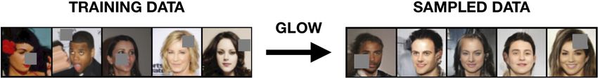
The above phenomenon is obtained by producing a disentangled representation in latent space. Dur-
ing the training procedure, the model simultaneously creates representations of objects with missing
parts and full images. The above factors are independent, and therefore we can sample from two
separated areas of latent space to produce full images and items with missing parts. The behavior is
presented in Fig. 1. We use the original Glow model with sampling temperature t = 0.7, for which
we should expect to appear about 60% of full images as shown in Tab. 1.
Figure 1: Missing Glow Phenomenon. Glow was trained on a missing dataset and then sampled with
temperature t = 0.7 (standard temperature for Glow), which gives about 60% of the full images.
The proposed approach’s main advantage is the ability to train a neural network on datasets con-
taining incomplete samples to produce a generative model on full images (the model does not see
any full images during training). This approach distinguishes it from recent models like denoising
autoencoder (Xie et al., 2012) or modified generative adversarial network (Yeh et al., 2017), which
require complete data as an input of the network in training.
In the paper, we show experiments that describe Missing Glow Phenomenon (see Section 3) and
present the theoretical explanation of such behaviors (see Section 4).
1Submitted to the ICLR 2021 Workshop on Geometrical and Topological Representation Learning
2 R ELATED WORKS
There is a rich literature on handling missing values (Little & Rubin, 2019). Theoretical guaran-
tees of estimation strategies or imputation methods rely on assumptions regarding the missing-data
mechanism, i.e., the cause of the lack of data. There are three mechanisms for the formation of miss-
ing data. Missing Completely At Random (MCAR) if the probability of being missing is the same
for all observations. Missing At Random (MAR) if the probability of being missing only depends
on observed values, and the last Missing Not At Random (MNAR) if the unavailability of the data
depends on both observed and unobserved data such as its value itself.
A classical approach to estimating parameters with missing values consists of maximizing the ob-
served likelihood, using, for instance, an Expectation-Maximization algorithm (Dempster et al.,
1977). One of its main drawbacks is to rely on strong parametric assumptions for the distributions
of the covariates. Another popular strategy to fix the missing values issue is predicting the missing
values based on observable ones, e.g., mean or k-NN imputation. One can also train separate mod-
els, e.g., neural networks (Sharpe & Solly, 1995), extreme learning machines (ELM) (Sovilj et al.,
2016), k-nearest neighbors (Batista et al., 2002).
In (Rubin, 1976), the appropriateness of ignoring the missing process when approach likelihood-
based or Bayesian inference was introduced and formalized. Under certain assumptions on the
missing mechanism, we can build a probabilistic model of incomplete data, which is subsequently
fed into a particular learning model (Liao et al., 2007; Dick et al., 2008; Śmieja et al., 2019).
A body of research on deep frameworks that can learn from partially observed data has emerged
in recent years. Initial work focused on extensions of generative models such as Variational Auto
Encoders (VAEs) (Kingma & Welling, 2013) and Generative Adversarial Networks (GANs) (Good-
fellow et al., 2014). In (Yoon et al., 2018) used generative adversarial net (GAN) to fill in absent
attributes with realistic values. In (Gupta et al., 2016) was proposed the supervised imputation,
which learns a replacement value for each missing attribute jointly with the remaining network pa-
rameters. This group also includes models such as the Missing Data Importance-Weighted Autoen-
coder (MIWAE) (Mattei & Frellsen, 2019), the Generative Adversarial Imputation Network (GAIN)
(Zhang et al., 2020), and the GAN for Missing Data (MIS-GAN) (Li et al., 2019). More recently,
the state-of-the-art benchmark on learning from incomplete data has been pushed by bidirectional
generative frameworks, which leverage the ability to map back and forth between the data space and
the latent space. Two such examples include the Monte-Carlo Flow model (MCFlow) (Richardson
et al., 2020) and the Partial Bidirectional GAN (PBiGAN) (Li & Marlin, 2020).
3 E XPERIMENTS
Missing dataset For the purpose of the experiments, we construct a special dataset with missings,
based on a CelebA - a large-scale dataset with more than 200K celebrities’ images annotated with
about 40 attributes (Liu et al., 2015). We resize each of the images into 64 × 64 pixels size and
impute a grey square box, which is a missing part of an image, as shown in Fig. 1 (left image).
The missing squares are placed at the beginning of the training, and their locations come from the
uniform distribution. Thus, the model always sees each of the original images with the square in the
same position. We used different sizes of missing squares in the following experiments - from 2 × 2
up to 20 × 20 pixels. Note that the small missing square (e.g. 2 × 2 or 4 × 4) could be seen as an
Figure 2: Reconstructed images for 20 × 20 missing dataset. Parameter α is a scaling factor of
original images’ representations in a latent space. For α = 1.0, we have an original missing image.
2Submitted to the ICLR 2021 Workshop on Geometrical and Topological Representation Learning
attribute by a model. Whereas images with the missing squares larger than 20 × 20 are, in fact, too
corrupted to recreate.
Glow model architecture In order to process the missing dataset properly, we use a powerful
flow-based model - Glow (Kingma & Dhariwal, 2018), where invertible 1 × 1 convolutions assure
invertibility. Glow is known for its competitive results among other flow models, e.g., RealNVP
(Dinh et al., 2016). For all of our experiments, we use the same Glow architecture with the following
hyperparameters: 4 blocks, 32 flows in each block, 5 bits, and 3 input channels.
Imputing missings We learned a Glow model on a specific missing dataset for each of the missing
squares’ sizes. In our setting, we use batch size 16 and 200k iterations. After training, we process the
data follow the procedure: (1) take image x from missing dataset; (2) create its latent representation
z with Glow by the embedding: z = Φ(x), where Φ : RN → − RN ; (3) move along the vector z in
a latent space by multiplying it by the parameter α. For α ∈ (0.0, 1.0] create a vector z 0 = αz; (4)
reconstruct imputed image x0 by the operation x0 = Φ−1 (z 0 ), which is the same as x0 = Φ−1 (αz)
for α ∈ (0.0, 1.0].
Figure 3: Images sampled from Glow with the temperatures t = 0.5, t = 0.6, and t = 0.7 (from
top to bottom) - in these regions of the latent space, Glow put good faces with a small number of
missing squares.
We present the partial results for the missing dataset with 20 × 20 missing boxes in Fig. 2. Glow
model was trained for 200k iterations, and we reconstruct the images by multiplying latent repre-
sentations by parameter α ∈ {0.1, 0.2, . . . , 1.0}. However, for parameter α in range (0.5, 0.7), the
reconstruction is actually an original image with an imputed missing part. Full results are presented
in Appendix.
Sampling from a latent representation All the previously introduced experiments were initial
parts for sampling images from Glow’s latent space with a specific temperature t.
We observe various behaviors in different parts of latent space. As shown in Fig. 3, the images
sampled with a temperature t ∈ (0.5, 0.7) are characterized by faces similar to the original ones
with a relatively small number of missing squares. On the other hand, Glow samples fuzzy images,
full of missing regions, when taking the temperatures t ≥ 1.0 (Fig. 4).
4 T HEORETICAL STUDIES
In this section, we are going to explain the Missing Glow Phenomenon showed in the experiments.
Let us recall that to sample from temperature t, we sample z in the latent and return Φ−1 (tz).
For intuition, consider the case when the data comes from the normal distribution N (0, Σ), and then
the flow can be chosen to be a linear function. Then by sampling from temperature t, we sample,
in fact, from the normal density N (0, t2 Σ). Consequently, for t going to zero, we sample from
the data with covariance converging to zero, while increasing t leads to the covariance increase.
Figure 4: Exemplary images sampled with the temperature t = 1.2. We observe that images in this
region are fuzzy and with a large number of missing boxes.
3Submitted to the ICLR 2021 Workshop on Geometrical and Topological Representation Learning
√
Moreover, if X ∼ N (0, Σ), then to sample from the temperature t = l, we can sample X1 , . . . , Xl
independently and return X1 + . . . + Xl . The last follows from the fact that the covariance of the
sum of independent random variables is the sum of their covariances.
Temperature t 0.1 0.2 0.3 0.4 0.5 0.6 0.7 0.8 0.9 1.0 1.1 1.2 1.3 1.4 1.5
frequency (%)
0 squares 100 100 100 98 92 70 64 56 50 42 30 30 24 22 22
1 square 0 0 0 2 8 26 30 34 38 44 54 44 46 46 44
2 squares 0 0 0 0 0 4 6 10 12 10 10 18 22 24 24
3 squares 0 0 0 0 0 0 0 0 0 4 4 4 4 4 6
4 squares 0 0 0 0 0 0 0 0 0 0 2 4 4 4 4
number of missing squares in the reconstruction image
Empirical E 0.00 0.00 0.00 0.02 0.08 0.34 0.42 0.54 0.62 0.76 0.94 1.08 1.18 1.22 1.26
Theoretical E 0.01 0.04 0.09 0.16 0.25 0.36 0.49 0.64 0.81 1.00 1.21 1.44 1.69 1.96 2.25
Table 1: Distribution of the number of missing squares when sampling with a specific temperature.
We provide both empirical and theoretical expected values E.
So let us now continue our discussion in the case when the data is an independent sum of two Gaus-
sian variables. Assume that the random vector X generating the data can be decomposed into the
sum of independent Gaussian random vectors: X = V+W. Then sampling from X with temperature
t is equivalent to sampling from V and W with temperature t.
Let us now try to interpret the above in the case of our experiment. Then X denotes the random
vector, which selects an image and then changes color to gray at the randomly chosen square of size
K × K. Thus we can interpret our model as the independent composition of two operations:
• V: sampling a random image from our original dataset,
• W: changing the color of the randomly chosen square of size K × K to gray.
√
Then sampling from V with temperature t = 2 is easy, as we simply sample two images, add their
latent representations, and process back to input space.
However, a crucial role is played by the operation W.
√ By applying the above reasoning informally,
we obtain that for covariance tCovW, where t = l, we obtain t2 times randomly covering by
squares of K × K. Extrapolating this formula for all t, we obtain the theoretical value for the
expected number of squares
E(number of missing squares | random sample from temperature t) = t2 .
For verification, we compare this with the values obtained in the experiments.
Ablation study Moreover, we provide an ablation study for the expected number of miss-
ing squares when sampling with a set temperature t and compare the results to the theo-
retical results. We sampled a set of 50 images for each of the temperatures and manually
calculated the number of missing squares. Then, we calculated empirical expected values
E(number of missing squares | random sample from temperature t) and compared them to the theo-
retical ones.
As shown in Tab. 1, the empirical expected number of missing squares is much different from
theoretical numbers. The reason for these dissimilarities is the fact that Glow models are weak and
imperfect learners. Moreover, we suppose that Glow’s restriction on the rigid representation could
cause such differences. However, we noticed similar expected numbers of missing squares for the
sampling temperature t = 0.7, which is the original Glow model (Kingma & Dhariwal, 2018), which
suggests that for such t, Glow fulfills its theoretical properties.
5 C ONCLUSION
In this paper, we show that flow-based generative models like Glow (Kingma & Dhariwal, 2018)
can be trained on images with missing data and produce full images without missing parts. The
above phenomenon is obtained by producing a disentangled representation in latent space. During
the training procedure, the model simultaneously creates representations of objects with missing
parts and full images. The above factors are independent, and therefore we can sample from two
separated areas of latent to produce full images and items with missing parts.
4Submitted to the ICLR 2021 Workshop on Geometrical and Topological Representation Learning
R EFERENCES
Gustavo EAPA Batista, Maria Carolina Monard, et al. A study of k-nearest neighbour as an imputa-
tion method. His, 87(251-260):48, 2002.
Arthur P Dempster, Nan M Laird, and Donald B Rubin. Maximum likelihood from incomplete data
via the em algorithm. Journal of the Royal Statistical Society: Series B (Methodological), 39(1):
1–22, 1977.
Uwe Dick, Peter Haider, and Tobias Scheffer. Learning from incomplete data with infinite impu-
tations. In Proceedings of the 25th international conference on Machine learning, pp. 232–239,
2008.
Laurent Dinh, Jascha Sohl-Dickstein, and Samy Bengio. Density estimation using real nvp. arXiv
preprint arXiv:1605.08803, 2016.
Ian Goodfellow, Yoshua Bengio, Aaron Courville, and Yoshua Bengio. Deep learning, volume 1.
MIT Press, 2016.
Ian J Goodfellow, Jean Pouget-Abadie, Mehdi Mirza, Bing Xu, David Warde-Farley, Sherjil
Ozair, Aaron Courville, and Yoshua Bengio. Generative adversarial networks. arXiv preprint
arXiv:1406.2661, 2014.
Maya Gupta, Andrew Cotter, Jan Pfeifer, Konstantin Voevodski, Kevin Canini, Alexander
Mangylov, Wojciech Moczydlowski, and Alexander Van Esbroeck. Monotonic calibrated in-
terpolated look-up tables. The Journal of Machine Learning Research, 17(1):3790–3836, 2016.
Diederik P Kingma and Prafulla Dhariwal. Glow: Generative flow with invertible 1x1 convolutions.
arXiv preprint arXiv:1807.03039, 2018.
Diederik P Kingma and Max Welling. Auto-encoding variational bayes. arXiv preprint
arXiv:1312.6114, 2013.
Steven Cheng-Xian Li and Benjamin Marlin. Learning from irregularly-sampled time series: A
missing data perspective. In International Conference on Machine Learning, pp. 5937–5946.
PMLR, 2020.
Steven Cheng-Xian Li, Bo Jiang, and Benjamin Marlin. Misgan: Learning from incomplete data
with generative adversarial networks. arXiv preprint arXiv:1902.09599, 2019.
Xuejun Liao, Hui Li, and Lawrence Carin. Quadratically gated mixture of experts for incomplete
data classification. In Proceedings of the 24th International Conference on Machine learning, pp.
553–560, 2007.
Roderick JA Little and Donald B Rubin. Statistical analysis with missing data, volume 793. John
Wiley & Sons, 2019.
Ziwei Liu, Ping Luo, Xiaogang Wang, and Xiaoou Tang. Deep learning face attributes in the wild.
In Proceedings of the IEEE international conference on computer vision, pp. 3730–3738, 2015.
Pierre-Alexandre Mattei and Jes Frellsen. Miwae: Deep generative modelling and imputation of
incomplete data sets. In International Conference on Machine Learning, pp. 4413–4423. PMLR,
2019.
Patrick E McKnight, Katherine M McKnight, Souraya Sidani, and Aurelio Jose Figueredo. Missing
data: A gentle introduction. Guilford Press, 2007.
Trevor W Richardson, Wencheng Wu, Lei Lin, Beilei Xu, and Edgar A Bernal. Mcflow: Monte
carlo flow models for data imputation. In Proceedings of the IEEE/CVF Conference on Computer
Vision and Pattern Recognition, pp. 14205–14214, 2020.
Donald B Rubin. Inference and missing data. Biometrika, 63(3):581–592, 1976.
Peter K. Sharpe and RJ Solly. Dealing with missing values in neural network-based diagnostic
systems. Neural Computing & Applications, 3(2):73–77, 1995.
5Submitted to the ICLR 2021 Workshop on Geometrical and Topological Representation Learning
Marek Smieja, Łukasz Struski, Jacek Tabor, Bartosz Zieliński, and Przemysław Spurek. Processing
of missing data by neural networks. In Proceedings of the 32nd International Conference on
Neural Information Processing Systems, pp. 2724–2734, 2018.
Marek Śmieja, Łukasz Struski, Jacek Tabor, and Mateusz Marzec. Generalized rbf kernel for in-
complete data. Knowledge-Based Systems, 173:150–162, 2019.
Dušan Sovilj, Emil Eirola, Yoan Miche, Kaj-Mikael Björk, Rui Nian, Anton Akusok, and Amaury
Lendasse. Extreme learning machine for missing data using multiple imputations. Neurocomput-
ing, 174:220–231, 2016.
Junyuan Xie, Linli Xu, and Enhong Chen. Image denoising and inpainting with deep neural net-
works. Advances in neural information processing systems, 25:341–349, 2012.
Raymond A Yeh, Chen Chen, Teck Yian Lim, Alexander G Schwing, Mark Hasegawa-Johnson, and
Minh N Do. Semantic image inpainting with deep generative models. In Proceedings of the IEEE
conference on computer vision and pattern recognition, pp. 5485–5493, 2017.
Jinsung Yoon, James Jordon, and Mihaela Schaar. Gain: Missing data imputation using generative
adversarial nets. In International Conference on Machine Learning, pp. 5689–5698. PMLR, 2018.
Yuxin Zhang, Zuquan Zheng, and Roland Hu. Super resolution using segmentation-prior self-
attention generative adversarial network. arXiv preprint arXiv:2003.03489, 2020.
6Submitted to the ICLR 2021 Workshop on Geometrical and Topological Representation Learning
A R ECONSTRUCTION IMAGES
In this section, we present the full results of imputing missings experiment. Dataset was con-
structed with 20 × 20 missing squares. Glow model was trained for 200k iterations, and we
reconstruct the images by multiplying missing images’ latent representations by parameter α ∈
{0.1, 0.2, 0.3, 0.4, 0.5, 0.6, 0.7, 0.8, 1.0}. Results are presented in Fig. 5.
Figure 5: Reconstructed images for 20 × 20 missing dataset. Parameter α was set to
{0.1, 0.2, 0.3, 0.4, 0.5, 0.6, 0.7, 0.8, 0.9, 1.0} from top to the bottom. For α = 1.0 (bottom image),
we have original missing data. Note that for the parameters in range (0.5, 0.7), the reconstruction is
actually an original image with an imputed missing part.
We observe that the latent space is constructed as follows: in the center, we can see the mean images
without missing parts. The further from the center, images are much more similar to the original
ones - faces are becoming the celebrities’ faces, and missing are starting to appear. However, we
observe that for α ∈ (0.5, 0.7), the reconstructed images have imputed missing squares and faces
very well correspond to the originals.
7Submitted to the ICLR 2021 Workshop on Geometrical and Topological Representation Learning
B H ISTOGRAMS OF THE NORMS IN LATENT SPACE
We also set the Glow model, which was trained on a specific missing dataset (e.g. 16 × 16). Then,
we checked the norm of the radiuses of latent representations z if the data came from the original
missing dataset or from a different one - i.e., with different sizes of missing squares (2 × 2, 8 × 8,
32 × 32) or a various number of missing squares of the same size (0, 1, 2). We also compare the
radiuses of latent representations of data that came from the original CelebA dataset (data with 0
missing squares or squares with size 0 × 0). From each dataset, we selected a batch of 100 images.
As presented in Fig. 6, we observe that the distributions of representations are similar for various
sizes of missing squares. The only exceptions are images with a missing square of size 2 × 2,
which are usually much further from the center of latent space. This behavior complies with the
reconstruction results - the missing square of size 2 × 2 is strange for the model cause it is too small
to be the missing part of an image attribute. However, the distribution for no missing squares is
similar to the others, suggesting that the imputed images are near the missing ones in a latent space.
We can see the same behavior for the different number of missing squares - distributions of the
original CelebA images are close to the distributions for missing datasets.
Figure 6: Histograms of the norm of radiuses of latent representation of the missing image. Glow
model was previously trained on 16 × 16 missing data. We tested this model with the data from
various missing datasets (2 × 2, 8 × 8, 16 × 16, 32 × 32) and original CelebA (0 × 0) - left plot.
Moreover, we tested also on data with the various number of missing squares: 0, 1, 2 - right plot.
8You can also read