Modelling DVFS and UFS for Region-Based Energy Aware Tuning of HPC Applications
←
→
Page content transcription
If your browser does not render page correctly, please read the page content below
1

                                                   Modelling DVFS and UFS for Region-Based
                                                   Energy Aware Tuning of HPC Applications
                                                                                    Mohak Chadha∗ , Michael Gerndt†
                                                           Chair of Computer Architecture and Parallel Systems, Technische Universität München
                                                                                   Garching (near Munich), Germany
                                                                            Email: mohak.chadha@tum.de, gerndt@in.tum.de
arXiv:2105.09642v1 [cs.DC] 20 May 2021

                                                                                                                           regulators and dynamic clock sources by hardware vendors and
                                            Abstract—Energy efficiency and energy conservation are one                     is part of operating systems [5].
                                         of the most crucial constraints for meeting the 20MW power                           In earlier Intel processor architectures either the uncore
                                         envelope desired for exascale systems. Towards this, most of
                                         the research in this area has been focused on the utilization                     frequency, i.e., frequency of uncore components (e.g. L3
                                         of user-controllable hardware switches such as per-core dynamic                   cache), was fixed (Nehalem-EP and Westmere-EP) or the core
                                         voltage frequency scaling (DVFS) and software controlled clock                    and uncore parts of the processor shared a common frequency
                                         modulation at the application level. In this paper, we present                    and voltage (Sandy Bridge-EP and Ivy Bridge-EP) [6]. In
                                         a tuning plugin for the Periscope Tuning Framework which                          new Intel processor architectures, i.e., Haswell onwards, a
                                         integrates fine-grained autotuning at the region level with DVFS
                                         and uncore frequency scaling (UFS). The tuning is based on                        new feature called uncore frequency scaling (UFS) has been
                                         a feed-forward neural network which is formulated using Per-                      introduced. UFS supports separate core and uncore frequency
                                         formance Monitoring Counters (PMC) supported by x86 systems                       domains and enables users to manipulate core and uncore
                                         and trained using standardized benchmarks. Experiments on five                    frequencies independently. Changing the uncore frequency has
                                         standardized hybrid benchmarks show an energy improvement                         a significant impact on memory bandwidth and cache-line
                                         of 16.1% on average when the applications are tuned according
                                         to our methodology as compared to 7.8% for static tuning.                         transfer rates and can be reduced to save energy [6], [7].
                                                                                                                              The Periscope Tuning Framework [8] is an online automatic
                                           Index Terms—Energy-efficiency, autotuning, dynamic voltage                      tuning framework which supports performance analysis and
                                         and frequency scaling, uncore frequency scaling, dynamic tuning
                                                                                                                           performance tuning of HPC applications. It also provides a
                                                                                                                           generic Tuning Plugin Interface which can be used for the
                                                                                                                           development of plugins. In this paper, we present a tuning
                                                                   I. I NTRODUCTION                                        plugin which utilizes PTF’s capability to manage search spaces
                                            Modern HPC systems consists of millions of processor cores                     and region-level optimizations to combine fine-grained auto-
                                         and offer petabytes of main memory. The Top500 list [1]                           tuning with hardware switches, i.e., core frequency, uncore
                                         which is published twice every year ranks the fastest 500                         frequency and OpenMP [9] threads. The applications are tuned
                                         general purpose HPC systems based on their floating point                         with node energy consumption as the fundamental tuning
                                         performance on the LINPACK benchmark. The published                               objective using a neural network [10] based energy model
                                         data indicates that the performance of such systems has been                      which is formulated using standardized PAPI counters [11]
                                         steadily increasing along with increasing power consump-                          available on Intel systems. After the completion of perfor-
                                         tion [2], [3]. The current fastest system delivers a performance                  mance analysis performed by PTF the tuning plugin generates
                                         of 122.30 PFlop/s while consuming 8.81MW of power. In                             a tuning model which contains a description of the best found
                                         order to achieve the 20MW power envelope goal for an                              hardware configurations, i.e., core frequency, uncore frequency
                                         exascale system as published by DARPA [4] we need 8.17                            and OpenMP threads for each scenario. A scenario consists
                                         fold increase in performance with only a 2.27 fold increase in                    of different regions which are grouped together if they have
                                         the power consumption.                                                            the same optimal configuration. This is commonly known as
                                            With the growing constraints on the power budget, it is                        System-Scenario methodology [12] and is extensively used in
                                         essential that HPC systems are energy efficient both in terms                     embedded systems. In order to evaluate our approach and the
                                         of hardware and software. Towards this, several power opti-                       accuracy of our tuning model we use the generated tuning
                                         mization techniques such as dynamic voltage and frequency                         model as an input for the READEX Runtime Library (RRL)
                                         scaling (DVFS), clock gating, clock modulation, ultra-low                         developed as part of the READEX project [13]. RRL enables
                                         power states and power gating have been implemented in state-                     dynamic switching and dynamically adjusts the system config-
                                         of-the-art processors by hardware vendors. DVFS is a common                       uration during application runtime according to the generated
                                         technique which enables the changing of the core frequency                        tuning model. Our key contributions are:
                                         and voltage at runtime. It reduces the processor’s frequency                         • We implement and evaluate a model based tuning plu-
                                         and voltage, resulting in reduced dynamic and static power                             gin for PTF with core frequency, uncore frequency and
                                         consumption and thus leads to energy savings depending on                              OpenMP threads as tuning parameters on HPC applica-
                                         the application characteristics. It is implemented using voltage                       tions.
                                         ©2019 IEEE. Personal use of this material is permitted. Permission from IEEE must be obtained for all other uses, in any current or future media, including
                                         reprinting/republishing this material for advertising or promotional purposes, creating new collective works, for resale or redistribution to servers or lists, or
                                         reuse of any copyrighted component of this work in other works.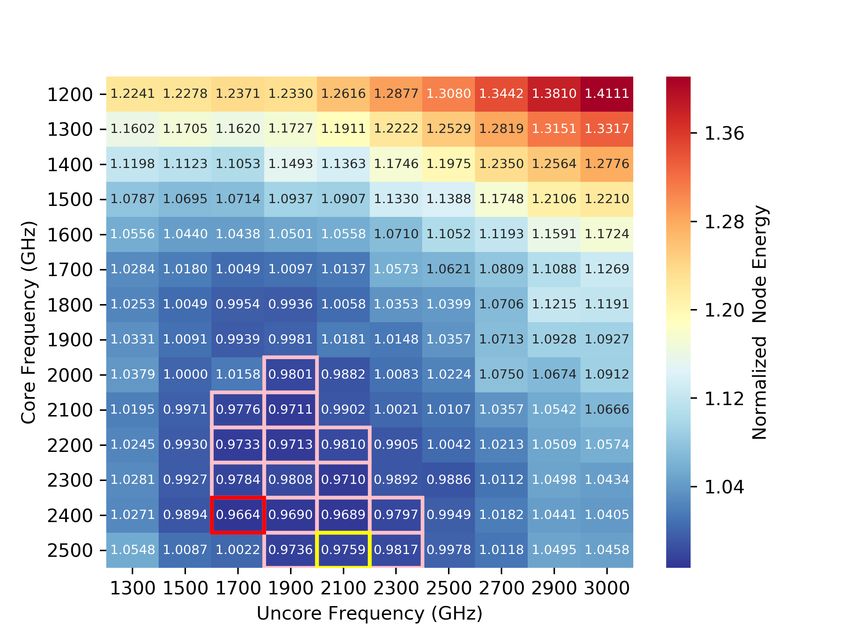
2

  •  We evaluate the accuracy of our model using sophisti-
     cated reference measurements conducted at high resolu-
     tion.
   • We practically demonstrate the viability of our methodol-
     ogy by comparing results for static and dynamically tuned
     applications and analyze performance-energy tradeoffs.
  The rest of the paper is structured as follows. Section II pro-
vides a background on auto-tuners and describes the existing
autotuning frameworks. In Section III, the tuning workflow
and implementation of the plugin are outlined. Section IV
describes the modeling approach and the model used by
the plugin. In Section V, the results of our approach are
presented. Finally, Section VI concludes the paper and presents
an outlook.

          II. BACKGROUND AND R ELATED W ORK                                Fig. 1: Overview of the Tuning Plugin Workflow

   A major challenge for several HPC applications is per-
formance portability, i.e., achieving the same performance           an exhaustive search for finding the best configuration of
across different architectures. State-of-the-art autotuners aim      tuning parameters, while in our approach we utilize an energy
to increase programmers productivity and ease of porting to          model to reduce the search space so as to select the optimal op-
new architectures by finding the best combination of code            erating core and uncore frequency which significantly reduces
transformations and tuning parameter settings for a given            the tuning time. Moreover in [7], each individual region needs
system and tuning objective. The application can either be           to be identified and manually instrumented to incorporate
optimized according to a single criteria, i.e., single objective     DVFS and UFS switching, while in our approach significant
tuning or across a wide variety of criteria, i.e., multi objective   region identification and application instrumentation are auto-
tuning. While this work focuses on energy consumption as the         matically achieved using readex-dyn-detect [13] and
tuning objective, other objectives such as total cost of own-        Score-P [21]. This allows our plugin to be used with any
ership (TCO), energy delay product (EDP) and energy delay            generic HPC application.
product squared (ED2P) can also be used. Furthermore, the
optimal configuration for tuning parameters can be determined                          III. T UNING W ORKFLOW
for an entire application, i.e., static tuning or individually for
                                                                        Figure 1. gives an overview of the different tuning steps
each region by changing the tuning parameters dynamically at
                                                                     involved in our tuning plugin workflow. The tuning of an
runtime, i.e., dynamic tuning. Since the search space created
                                                                     application is primarily a four step process comprising of
can be enormous, most autotuning frameworks utilize iterative
                                                                     pre-processing, determination of optimal number of OpenMP
techniques or analytical models to reduce the search space.
                                                                     threads, prediction of core and uncore frequencies for search-
   For optimizing parallel applications several autotuning
                                                                     space reduction and tuning model generation. Steps one to four
frameworks which target different tuning parameters such as
                                                                     are offline and constitute the design time analysis (DTA) of
compiler flags [14], [15] and application specific parame-
                                                                     the application. The production run which involves dynamic
ters [16] have been proposed. MATE [17] and ELASTIC [18]
                                                                     tuning using RRL [13] is online and involves a lookup in the
are two autotuning frameworks which support dynamic tuning
                                                                     generated tuning model. This section describes each step in
of MPI based parallel applications. However, their approach
                                                                     detail.
is more coarse grained as compared to the one introduced in
this paper using PTF [8].
   While most autotuning frameworks focus on improving               A. Pre-processing
time-to-solution, some frameworks also support tuning of                The Periscope Tuning Framework [8] utilizes the mea-
applications so as to improve energy efficiency [19], [20].          surement infrastructure for profiling and online analysis of
Most of these techniques involve the use of DVFS. Guillen et         HPC applications provided by Score-P [21]. The first step
al. [20] propose an automatic DVFS tuning plugin for PTF [8]         involves compiler instrumentation of program functions, MPI
which supports tuning of HPC applications at a region level          and OpenMP regions using Score-P. This inserts measure-
with respect to power specialized tuning objectives. The plugin      ment probes into the application’s source code and can often
reduces the search by using analytical performance models and        lead to overheads during application execution. In order to
selects the optimal operating core frequency. Sourouri et al. [7]    reduce overhead, we filter the application using the tool
propose an approach for dynamic tuning of HPC applications           scorep-autofilter developed as part of the READEX
with respect to energy based tuning objectives. Similar, to this     project [13]. Filtering is a two step process and involves run-
work their approach selects the optimal operating core, uncore       time and compile-time filtering. Executing the instrumented
frequency and the optimal number of OpenMP threads for tun-          application with profiling enabled creates a call-tree appli-
ing the application. However, the proposed approach involves         cation profile in the CUBE4 format [22]. The application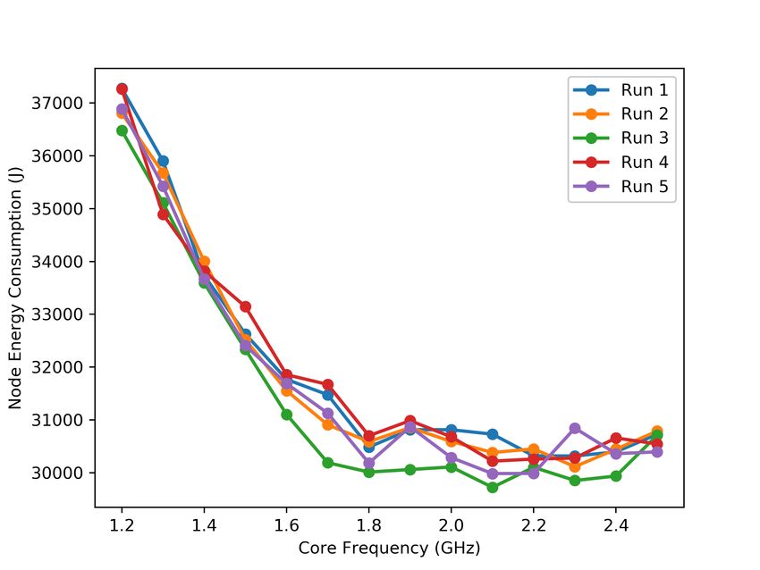
3

profile is then utilized during run-time filtering to generate       as the global core and uncore frequency. Global core and
a filter file which contains a list of finer granular regions        uncore frequency represent the optimal frequencies for the
below a certain threshold. The generated filter file is then used    phase region and constitute the reduced search space. This
to suppress application instrumentation during compile-time          highlights the main advantage of our modeling approach since
filtering. An alternative method of reducing overhead is by          we determine the optimal global core and uncore frequency in
using manual instrumentation. This requires analysis of the          one tuning step. Alternatively, the global operating core and
application profile generated by Score-P followed by manual          uncore frequencies can also be determined by exhaustively
annotation of the regions.                                           searching through the parameter space. However, this signifi-
    Following this, we manually annotate the phase region of         cantly increases the tuning time. We use the immediate neigh-
the application using specialized macros provided by Score-P.        boring frequencies of the global core and uncore frequency to
The phase region is a single entry, exit region which constitutes    verfiy and select the operating core and uncore frequencies for
one iteration of the main program loop. The application is           all significant regions. PTF utilizes the Score-P cpu_freq2
then executed to generate an application profile which is then       and uncore_freq3 PCP plugins [13] to dynamically change
used by the tool readex-dyn-detect [13] to identify the              core and uncore frequencies at runtime.
different significant regions present in the application. A region
qualifies as a significant region if it has a mean execution         D. Tuning Model Generation
time of greater than 100ms. Since energy measurement and
application of core and uncore frequencies has a certain                After all experiments are completed and different system
delay a threshold of 100ms is selected to ensure that the            configuration parameters have been evaluated, the tuning plu-
right execution time influenced by setting the frequencies is        gin generates the tuning model. To avoid dynamic-switching
measured. Readex-dyn-detect generates a configuration                overhead, regions which behave similar during execution or
file containing a list of significant regions which is used as an    have the same configuration for different tuning parameters are
input for the tuning plugin.                                         grouped into scenarios by the plugin. This is done by using a
                                                                     classifier which maps each region onto a unqiue scenario based
                                                                     on its context. Each scenario lists the best found configuration
B. Tuning Step 1: Tuning OpenMP threads                              of the hardware tuning parameters core frequency, uncore
   For tuning OpenMP and hybrid applications, the tuning             frequency and OpenMP threads. The generated tuning model
plugin supports the number of OpenMP threads as a tuning             is then used as an input for RRL [13] (see Section V-D) for
parameter. The lower bound and step size for the tuning              Runtime Application Tuning (RAT).
parameter can be specified in the configuration file generated
at the end of the pre-processing step (see Section III-A). We                        IV. M ODELLING M ETHODOLOGY
use an exhaustive approach to determine the optimal number              Chadha et al. [24] adapt and describe a statistically rig-
of OpenMP threads (see Figure 1). The tuning plugin creates          orous approach to formulate regression based power models
scenarios depending upon the input in the configuration file,        for high performance x86 Intel systems, originally used for
which are then executed and evaluated by the experiments en-         ARM processors [25]. The formulated models are based on
gine. In order to dynamically change the number of OpenMP            DVFS frequencies and standardized PAPI [11] counters. In
threads at runtime for each experiment, PTF utilizes the             this paper, we extend their work to formulate energy models
Score-P OpenMPTP1 Parameter Control Plugin (PCP) [13].               using a neural network architecture. This section describes our
The optimal number of OpenMP threads for each region                 modelling approach in detail.
are determined with energy consumption as the fundamental
tuning objective. To obtain energy measurements we use the
High Definition Energy Efficiency Monitoring (HDEEM) [23]            A. Data Acquisition
infrastructure. HDEEM provides measurements at a higher                 Similar to [24], we use standardized PAPI counters for
spatial and temporal granularity with a sampling rate of (1          formulating our energy model. The first step involves the
kSa/s) and leads to more accurate results. Energy measurement        collection of these performance metrics and energy values for
using HDEEM has a delay of 5 ms on average.                          different HPC applications. The obtained PAPI counter values
                                                                     are then utilized to select an optimal subset of counters. We
C. Tuning Step 2: Tuning Core and Uncore frequencies                 use the optimal PAPI counters as input for our energy model.
                                                                        In order to obtain PAPI counter values, along with en-
   Following the determination of optimal number of OpenMP           ergy information for different standardized benchmarks we
threads, the tuning plugin requests the appropriate performance      utilize the application tracing infrastructure provided by
metrics for the phase region (see Section IV-B) in the analysis      Score-P [21]. We use Score-P’s built-in support for obtaining
step as shown in Figure 1. These performance metrics are then        performance metrics to add PAPI data to the application
used as an input for the energy model in the tuning plugin           trace. The energy values are added to the trace by using
to predict energy consumption for different core and uncore          scorep_hdeem_plugin4 which implements the Score-P
frequencies. The combination of core and uncore frequency
which leads to the minimum energy consumption is then used             2 https://github.com/readex-eu/PCPs/tree/release/cpufreq   plugin
                                                                       3 https://github.com/readex-eu/PCPs/tree/release/uncorefreq   plugin
  1 https://github.com/readex-eu/PCPs/tree/release/openmp   plugin     4 https://github.com/score-p/scorep   plugin hdeem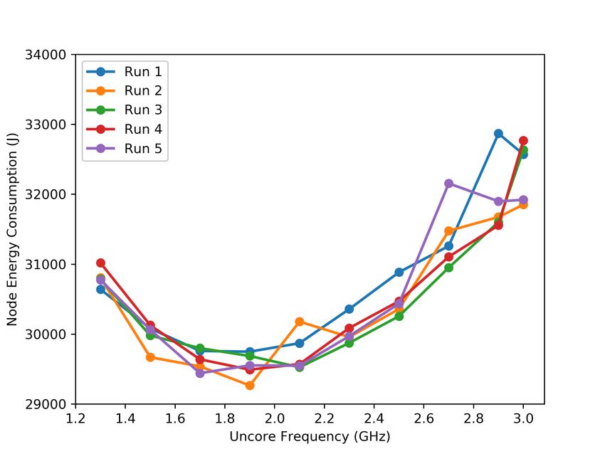
4

             (a) Node energy consumption with changing                       (a) Node energy consumption with changing
             core frequency.                                                 ucore frequency.

             (b) Normalized node energy consumption                          (b) Normalized node energy consumption
             with changing core frequency.                                   with changing uncore frequency
Fig. 2: Comparison of node and normalized node energy con-         Fig. 3: Comparison of node and normalized node energy con-
sumption for the benchmark Lulesh across different compute         sumption for the benchmark Lulesh across different compute
nodes when uncore frequency is fixed.                              nodes when core frequency is fixed.

                                                                   B. Model Parameter Selection
metric plugin interface. The performance metrics and energy           A common pitfall of energy modelling is power variability
values are recorded only at entry and exit of a region. The        among different compute nodes [27]. To examine this issue
applications are then executed to generate the application trace   we consider two scenarios:
in Open Trace Format 2 (OTF2) [26] format. The application           1) We vary the core frequency while keeping uncore fre-
trace consists of trace records sorted in a chronological order.        quency and OpenMP threads fixed at 1.5GHz and 24
To obtain energy values and performance metrics from appli-             respectively.
cation traces we implement a custom OTF25 post-processing            2) We vary the uncore frequency while keeping the core
tool. Our tool reports energy values for the entire application         frequency and OpenMP threads fixed at 2.0GHz and 24
run, while PAPI values are reported individually for instances          respectively.
of the phase region.                                                  Scenarios 1 and 2 are shown for the benchmark Lulesh,
   Our experimental platform (see Section V-A) supports 56         executed with one MPI process and 24 OpenMP threads on
standardized PAPI counters along with 162 native counters.         our experimental platform (see Section V-A) in Figure 2a and
Each native counter has many possible different configura-         Figure 3a respectively. Each run in Figure 2a and Figure 3a
tions. We focus on the standardized PAPI counters to keep          indicates execution of the workload on a separate compute
the amount of measurements needed feasible. For obtaining          node multiple times with changing core and uncore frequency.
values of all 56 PAPI counters, multiple runs of the same          The actual energy values of the application depend upon
application are required due to hardware limitations on the        the compute node where the application is being executed
simultaneous recording of multiple performance metrics. The        as shown in Figure 2a and Figure 3a. To account for the
energy and PAPI counter values are averaged across all runs.       issue of power variability, we normalize the energy values
The core and uncore frequency values are fixed to 2.0GHz           of a particular run with energy value obtained at 2.0GHz,
and 1.5 GHz for all measurements. Furthermore, we fix the          1.5GHz core and uncore frequency respectively. This reduces
OpenMP threads to 24 for OpenMP and hybrid applications            the variability across runs on different compute nodes as
(see Table II).                                                    shown in Figure 2b and Figure 3b. As a result of this, we
                                                                   train our model to predict normalized energy Enorm .
                                                                      Chadha et al. [24] describe an algorithm for selecting
                                                                   optimal PAPI counters for formulating regression based power
  5 https://github.com/kky-fury/OTF2-Parser                        models. The algorithm takes the entire set of standardized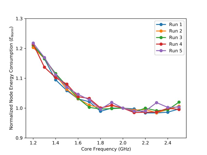
5

TABLE I: Selected performance counters based on all work-
                                                                           I1
loads.
                                                                                            H1       H1
                   Counter
                   BR NTK
                                 mean VIF
                                    n/a
                                                                           I2
                                                                                            .. ..
                                                                                ..
                    LD INS        1.068
                    L2 ICR
                   BR MSP
                                  1.460
                                  1.587
                                                                           I3
                                                                                             . .
                                                                                            H5       H5
                                                                                                              EN orm

                   RES STL
                    SR INS
                   L2 DCR
                                  2.405
                                  2.941
                                  3.065                                    I9    .
                                                                           Fig. 4: Used neural network architecture
PAPI counters, obtained for a given set of workloads as
input and returns an optimal set of counters. The counters
are selected by formulating regression models between the        This is primarily done to further reduce multicollinearity
PAPI counters and the dependent variable (power). We use         between the input features and to prevent one feature from
the same algorithm for selecting optimal PAPI counters for       dominating the model’s objective function. The mean and
our model with normalized node energy as the dependent           scaling information is determined from the applications in
variable. The authors also suggest the use of a heuristic        our training set (see Section V). PAPI counters are further
criterion called Variance Inflation Factor (VIF) to quantify     normalized by dividing them with the execution time of one
multicollinearity between the chosen PAPI counters. A large      phase iteration as each application can have single or multiple
mean VIF value, usually greater than 10 indicates that the       phase iterations.
selected events are related to each other [28]. Collinearity        We use the Rectified Linear Units (ReLU) [30] as activation
between the selected events is a common pitfall of power         functions in our neural network. This is because usage of
and energy modelling [29]. To formulate stable models, it        ReLU has been proven to lead to faster convergence [31] and
is essential that the selected counters are independent of       they overcome the problem of vanishing gradients. The ReLU
each other so that the model can have maximum information        units are placed before the two hidden layers and before the
regarding the workloads.                                         output layer.
   To select the optimal counters for formulating our energy        We initialize the weights of the neurons in the network by
model, we run the standardized benchmarks (see Table II)         randomly sampling from a zero mean,   p unit standard devia-
on one compute node of our experimental platform (see            tion Gaussian and multiplying with (2.0/n), as suggested
Section V-A) with the system configuration described in          by [32]. Here n represents number of neurons in the particular
Section IV-A. The optimal selected counters are shown in         layer. This improves the rate of convergence and ensures
Table I. The values of the selected counters depend only         that all neurons in the network initially have approximately
on the application characteristics and not on the frequen-       the same output distribution. The biases of the neurons are
cies. Hence any value of core and uncore frequency can be        initialized to zero. We use mean squared error as the objective
used for all measurements. The obtained mean VIF for the         function for training our model. The network predicts nor-
selected counters is low indicating limited multicollinearity    malized energy Enorm for a given set of PAPI counters, core
between the selected events. In Table I, BR_NTK describes        and uncore frequency. In order to predict the global operating
the total number of conditional branch instructions not taken,   core and uncore frequency as described in Section III-C, all
LD_INS describes the total number of load instructions,          combination of available frequencies are used as input to
L2_ICR describes the total number of L2 instruction cache        the network. The core and uncore frequency which leads to
reads, BR_MSP describes the total number of mispredicted         minimum energy consumption is then selected.
conditional branch instructions, RES_STL describes the total
number of cycles stalled on any resource, SR_INS describes                       V. E XPERIMENTAL R ESULTS
the total number of store instructions and L2_DCR describes        In this section, we describe the system used for training and
the total number of L2 data cache reads.                         validating our energy model. We present results to demonstrate
                                                                 the accuracy of our models, compare static and dynamic tuning
C. Neural Network Architecture                                   of applications and analyze energy performance trade-offs.

   To formulate our energy model we use a 2-layer fully-
connected neural network architecture as shown in Figure 4.      A. System Description
The input layer consists of nine neurons, followed by two           For our experiments, we use the Bull cluster Taurus [33]
hidden layers consisting of five neurons and one neuron at       located at Technische Universität Dresden (TUD) in Germany.
the output layer. The PAPI counters shown in Table I along       Taurus consists of six compute islands comprising of dif-
with the operating core and uncore frequencies constitute the    ferent Intel CPUs and Nvidia GPUs. Our experiments were
input features of our model. We standardize and center our       performed on the haswell partition which consists of 1456
input data by removing the mean and scaling to unit variance.    compute nodes based on Intel Haswell-EP architecture. Each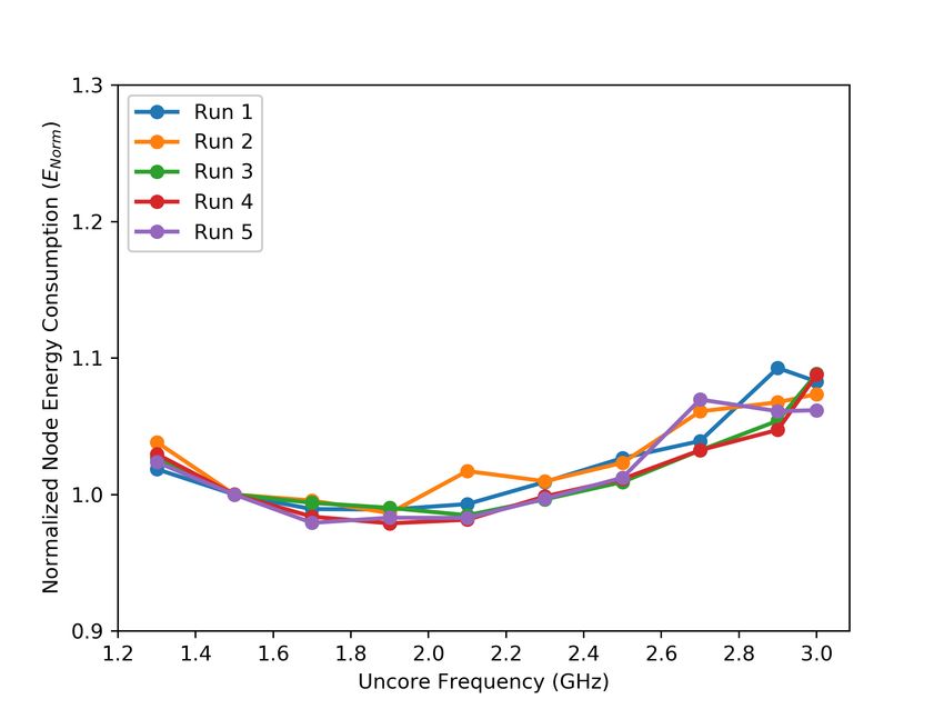
6

Fig. 5: Mean absolute (%) error for 19 benchmarks across DVFS and UFS states when the network is trained using LOOCV
                                                       technique.

         TABLE II: Benchmarks used for validation              bullxmpi1.2.8.4. We ran all the applications on one
      Suite                        Benchmarks                  compute node of our experimental platform for all supported
     NPB-3.3        CG, DC, EP, FT, IS, MG, BT, BT-MZ, SP-MZ   core frequencies and respectively uncore frequencies (see
                            Amg2013, Lulesh, miniFE,           Section V-A) to generate Score-P OTF2 [26] traces. For
    CORAL
                      XSBench, Kripke, Mcbenchmark (Mcb)       OpenMP and hybrid applications we vary the number of
     Mantevo                     CoMD, miniMD                  OpenMP threads from 12 to 24 with a granularity of 4.
    LLCBench                         Blasbench                 The generated traces are then post-processed to obtain
      Other                           BEM4I                    energy information as described in Section IV-A. The core
                                                               and uncore frequencies are changed by using the low-level
                                                               x86 adapt [39] library. We use 2.0GHz, 1.5GHz core and
compute node has two sockets, comprising of two Intel Xeon     uncore frequency respectively for calibrating our energy
E5-2680v3 processors with 12 cores each and total 64GB of      model. The energy values are normalized by using the
main memory. Hyper-Threading and Turbo Boost are disabled      energy value of the particular application at the calibrating
on the system. The core frequency of each cpu core ranges      frequencies. Furthermore, the PAPI counter values obtained at
from 1.2GHz to 2.5GHz, while the uncore frequency of the       the calibrating frequencies are used as input for the network.
two sockets ranges from 1.3GHz to 3.0GHz. Each compute            In order to evaluate the stability and performance of our
node is water cooled and is integrated with high resolution    model across unseen benchmarks we first train our network us-
HDEEM [23] energy monitoring infrastructure. While running     ing the technique Leave-one-out cross-validation (LOOCV). In
experiments, the energy measurements are obtained by using     each step of LOOCV a single benchmark forms the testing set
an FPGA integrated into the compute node which avoids per-     while the remaining benchmarks are used to train the network
turbation and leads to high accuracy of energy measurements.   (see Table II). This step is repeated for all benchmarks. To
                                                               train our network we use the stochastic optimization method
B. Neural Network Training                                     ADAM [40], which improves the rate of convergence. We use
   For training and validating our energy model experimen-     the default parameters of ADAM and a learning rate of 1e−3
tally, we use a wide variety of benchmarks from the NAS        for training our network. In each LOOCV step, the neural
Parallel Benchmark (NPB) suite [34], the CORAL benchmark       network is trained for five epochs, i.e. the neural network sees
suite [35], the Mantevo benchmark suite [36], LLCBench [37]    each training sample five times during forward and backward
benchmark suite and a real world application BEM4I [38]        pass. Increasing the number of epochs greater than five leads
which solves the Dirichlet boundary value problem for the 3D   to over-fitting and does not increase the accuracy of the model.
Helmholtz equation. The individual benchmarks are shown in     Figure 5 shows the mean absolute (%) error (MAPE) for all
Table II. The benchmarks selected from NPB except BT-MZ        benchmarks (see Table II) across all DVFS and respectively
and SP-MZ along with miniFE (see Table II) are implemented     UFS states. We obtain a maximum MAPE value of 9.35 for the
using OpenMP. We use MPI only versions of the benchmarks       benchmark miniMD and a minimum MAPE value of 2.81 for
Kripke and CoMD. All other benchmarks are implemented          the benchmark Lulesh. Our energy model achieves an average
using both MPI and OpenMP, i.e., hybrid.                       MAPE value of 5.20 for all benchmarks as compared to 7.54
   To collect energy information at the different core and     achieved by the regression based power model, trained using
uncore frequencies, the applications are instrumented          10-fold CV with random indexing in our previous work [24].
using Score-P and compiled using gcc7.16 and                   A disadvantage of 10-fold CV is that some benchmarks might
                                                               be repeated in both training and testing set. This indicates
 6 Compiler   flags: -m64 -mavx2 -march=native -O3             the stability and robustness of our energy model. Moreover,
7
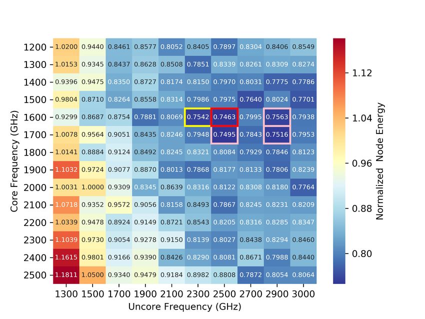
Fig. 6: Normalized node energy values for Lulesh for Fig. 7: Normalized node energy values for Mcbenchmark for
different core and uncore frequencies and 24 OpenMP different core and uncore frequencies and 20 OpenMP
threads. threads.
TABLE III: Obtained optimal configuration for different sig- TABLE IV: Obtained optimal configuration for different sig-
nificant regions of Lulesh nificant regions of Mcbenchmark
Region OpenMP CF UCF Region OpenMP CF UCF
threads (GHz) (GHz) threads (GHz) (GHz)
IntegrateStressForElems 24 2.50 2.00 setupDT 24 1.60 2.30
CalcFBHourglassForceForElems 24 2.50 2.00 advPhoton 24 1.60 2.30
CalcKinematicsForElems 24 2.40 2.00 omp parallel:423 20 1.60 2.30
CalcQForElems 24 2.50 2.00 omp parallel:501 20 1.70 2.20
ApplyMaterialPropertiesForElems 20 2.40 2.00 omp parallel:642 24 1.60 2.30
tuning for energy using regression would require two separate configuration selected by the tuning plugin 2.5|2.1 GHz
power and time models with core and uncore frequencies as (CF|UCF) as yellow and configurations withing 2% of the
independent variables, while this is accomplished by a simple minimum as pink. Since, the normalized node energy values
2-layer neural network as shown in this work. for different configuration of core and uncore frequencies (see
Following this, we test our model for the hybrid benchmarks Figure 6) are very close to the optimum, the actual energy
Lulesh, Amg2013, miniMD, BEM4I and Mcbenchmark and values can vary across compute nodes and configurations
train using the rest. The neural network is trained for 10 which are not the most optimal can result in energy savings.
epochs with the same hyper-parameters used for LOOCV. The benchmark Lulesh consists of five significant regions
In this scenario, we achieve a MAPE value of 7.80 for the which are determined using readex-dyn-detect [13] (see
benchmarks in the test set. The weights and biases of the Section III-A). The significant regions are different functions
trained network are then used in the tuning plugin for region in Lulesh, names of which are shown in Table III. Following
level tuning. the selection of the optimal configuration for the phase region,
the tuning plugin defines a reduced search space by using the
C. Region-level tuning frequencies in the immediate neighborhood of 2.5|2.1 GHz
The applications in the test set are instrumented with and generates scenarios. The OpenMP threads are fixed to
Score-P, pre-processed (see Section III-A) and then executed the optimum obtained for the phase region. The scenarios are
using PTF. We explicitly set the core and uncore frequency executed and evaluated by the experiments engine. The best
to the calibrating frequencies as described in Section V-B and found configuration for each significant region based on energy
run the applications with one MPI process and 24 OpenMP consumption is then selected. The best found configuration for
threads. For the first tuning step (see Section III-B) we use each region is shown in Table III.
a lower bound and step size of 12 and 4 OpenMP threads The tuning plugin determines the configuration 16 OpenMP
respectively. threads, 2.4|2.3 (CF|UCF) as the most optimal for the
For the benchmark Lulesh the tuning plugin determines 24 benchmark Amg2013 which consists of three significant re-
OpenMP threads as the optimum for the phase region. Figure 6 gions. For the benchmark miniMD which also consists of
shows the normalized node energy values for Lulesh at differ- three significant regions the configuration 24 OpenMP threads,
ent core and uncore frequencies and 24 OpenMP threads. With 2.4|2.0 (CF|UCF) is found to be the most optimal. For the
energy consumption as the fundamental tuning objective, Fig- real world application BEM4I consisting of four significant
ure 6 shows a trend towards higher core frequency and lower regions, the configuration 24 OpenMP threads, 2.4|2.4
uncore frequency indicating that Lulesh is compute-bound. In (CF|UCF) is found to be the most optimal by the tuning plugin.
Figure 6 we highlight the best found configuration 2.4|1.7 While the above discussed benchmarks are compute bound,
GHz (core frequency (CF)|uncore frequency (UCF)) as red, the Mcbenchmark is predominantly memory bound. Figure 78
TABLE V: Obtained optimal static configuration OpenMP threads and 2.5|3.0 GHz (CF|UCF) on a compute
Benchmark OpenMP CF UCF node. Following this, we manually set the best obtained static
threads (GHz) (GHz) configuration (see Table V) and execute the benchmark on
Lulesh 24 2.40 1.70 the same compute node. Savings in terms of job energy, CPU
Amg2013 16 2.50 2.30 energy and time are then computed relative to the values for
miniMD 24 2.50 1.50 the default configuration.
BEM4I 24 2.30 1.90 Following the tuning model generation in the previous step
Mcbenchmark 20 1.60 2.50 for the five instrumented benchmarks, we use the tuning model
as an input for the RRL7 [13] library. This is done by using
the environment variable SCOREP_RRL_TMM_PATH. RRL
shows a trend towards higher uncore frequency and lower core enables runtime application tuning and uses the Score-P PCP
frequency indicating the need for higher memory bandwidth. plugins to dynamically change the system configuration at run-
The tuning plugin determines 20 OpenMP threads, 1.6|2.3 time. The configuration applied is extracted from the different
GHz (CF|UCF) as the optimal configuration of the phase re- scenarios in the generated tuning model (see Section III-D).
gion as compared to the optimum at 1.6|2.5 GHz (CF|UCF) The job energy, CPU energy and time values at the end of the
as shown in Figure 7. Mcbenchmark consists of five significant RRL run are then used to compute dynamic savings relative to
regions, two functions and three OpenMP parallel constructs. the parameter values for the default configuration. The values
The optimal configuration for each significant region is shown for both static and dynamic savings are averaged over five
in Table IV. At the end of the PTF run the tuning plugin runs.
generates the tuning model by grouping regions with similar Table VI shows the static and dynamic tuning savings for the
configuration into scenarios as described in Section III-D. five benchmarks. For static tuning we achieve average savings
In order to quantify the tuning time in our approach as of 3.5%, 7.8% in terms of job and CPU energy respectively.
compared to the one introduced in [7], consider the workload On the other hand, when the benchmarks are dynamically
Mcbenchmark with n regions. Suppose that one run of the tuned using our methodology, average energy improvement
benchmark takes t sec and the search space for finding the of 7.53%, 16.1% for job and CPU energy is observed. The
optimal configuration, i.e., OMP|CF|UCF is k x l x m. Since increase in energy savings can be attributed to the selection
the approach introduced in [7] does not consider significant of only certain regions above a threshold as significant (see
regions and uses an exhaustive search policy, the tuning time Section III-A) and the usage of scenarios in the tuning model.
would be n x k x l x m x t. However, since we tune all Maximum energy improvement of 10.3%, 21.95% in terms
significant regions in a single application run and use an for job and CPU energy is observed for the dynamically
energy model in our approach, the tuning time is significantly tuned benchmark miniMD, while minimum is observed for
reduced to (k + 1 + 9) x t as discussed in Section III. Moreover, the benchmark Lulesh with static tuning (see Table VI).
in applications with progressive loops such as Lulesh each Static tuning leads to a slight improvement in performance
phase iteration can be exploited and the entire application run for the benchmarks Lulesh, miniMD and BEM4I, while the
is not required. In that case, the tuning time would be (k + 1 performance is decreased for the benchmarks Amg2013 and
+ 9). Mcbenchmark. For Amg2013 the decrease in performance can
be attributed to the optimal static configuration of 16 OpenMP
D. Comparing Static and Dynamic Tuning threads as compared to 24 for the default configuration. In case
To compare static and dynamic tuning, we consider three of Mcbenchmark the increase in execution time is primarily
parameters job energy, CPU energy and time. To measure due to the optimal low operating core frequency value of 1.6
job energy and time, we use the SLURM tool sacct which GHz (see Table V) in comparison to 2.5 GHz for the default
allows users to query post-mortem job data for any previously configuration.
executed jobs or job steps. The energy and time values can be
obtained by using the --format parameter. For measuring E. Analyzing Overhead
CPU energy we utilize a lightweight runtime tool called Although dynamic tuning is more energy efficient, it leads to
measure-rapl which uses the x86 adapt [39] library to a decrease in performance as shown in Table VI. The decrease
measure the CPU energy via Intel’s RAPL interface. in performance is because of three reasons. First, reduction in
Table V shows the optimal static configuration found for performance due to configuration setting. Second, overhead
each benchmark. These values are obtained by running the due to dynamic switching. Third, instrumentation overhead
benchmarks at different OpenMP threads, core frequencies due to Score-P. To quantify the performance reduction due
and uncore frequencies. The configuration which results in to the configuration setting, we measure the relative execution
minimum energy consumption is then selected. The best found time of each reach region w.r.t the default configuration for
static configuration is equivalent to the best configuration each benchmark. The values found are shown in Table VI.
found for the phase region. The default operating core and To change the core and uncore frequencies the Score-P PCP
uncore frequency for any job running on our experimental plugins utilize the x86 adapt [39] library. The transition
platform (see Section V-A) is 2.5|3.0 GHz (CF|UCF). In latency for changing frequency of one individual core on our
order to compute static savings for a particular benchmark, the
benchmark is first executed with a default configuration of 24 7 https://github.com/readex-eu/readex-rrl9
TABLE VI: Static and Dynamic Tuning Results
Static tuning savings Dynamic tuning savings
Benchmark job energy/CPU energy/time job energy/CPU energy/time/performance overhead DVFS/UFS/Score-P
reduction config setting
Lulesh 1.14%/2.60%/0.97% 5.48%/10.30%/−7.70%/−5.46% −2.24%
Amg2013 4.89%/12.63%/−6.80% 5.42%/16.67%/−11.2%/−8.96% −2.24%
miniMD 4.10%/8.63%/0.41% 10.3%/21.95%/−4.00%/−2.29% −1.71%
BEM4I 2.64%/4.61%/0.70% 8.26%/12.43%/−4.25%/−2.98% −1.27%
Mcbenchmark 6.00%/10.50%/−6.50% 8.20%/18.76%/−14.50%/−10.10% −4.40%
experimental platform is 21µs, while changing the operating technique Leave-one-out-cross-validation, achieving an aver-
uncore frequency for each socket has a transition latency of age MAPE value of 5.20 for all DVFS and respectively UFS
20µs. Without considering scenarios, the DVFS/UFS overhead states.
for a particular benchmark can be computed by multiplying We present results for region based tuning of five hybrid
the number of iterations with the number of significant regions applications. Moreover, we demonstrate the viability of our
and the transition latency. Although runtime and compile-time approach by comparing static and dynamically tuned ver-
filtering along with manual instrumentation (see Section III-A) sions of the applications. For dynamic tuning we utilize the
reduce Score-P overhead to a large extent, it is not completely READEX Runtime Library (RRL) which dynamically changes
removed due to instrumentation of OpenMP and MPI routines the system configuration at runtime. Our experiments show an
by Score-P. The combined DVFS/UFS/Score-P overhead in energy improvement of 7.53%, 16.1% in terms of job and
our approach ranges from 20-30.34% for the five benchmarks CPU energy for dynamically tuned applications as compared
(see Table VI) as compared to 10-50% in [7]. to 3.5%, 7.8% for static tuning.
In the future we want to investigate the application of the
model based approach to individual significant regions. By
VI. C ONCLUSION & F UTURE W ORK that regions with a very different best configuration could be
Energy-efficiency of current as well as future HPC systems identified, e.g., IO regions. Furthermore, we would like to add
remains a key challenge due to their increasing number of support for other energy based tuning objectives such as EDP,
components and complexity. As a result, several techniques ED2P.
which utilize dynamic voltage and frequency scaling, software
VII. ACKNOWLEDGMENT
clock modulation and power-capping to tune and reduce the
energy consumption of applications have been developed. The research leading to these results was partially funded by
However, most of these techniques either require extensive the European Union’s Horizon 2020 Programme under grant
manual instrumentation or tune the applications statically. In agreement number 671657 and Deutsche Forschungsgemein-
this paper, we have developed a tuning plugin for the Periscope schaft (DFG, German Research Foundation)-Projektnummer
Tuning Framework which utilizes user-controllable hardware 146371743-TRR 89: Invasive Computing. We thank the Centre
switches, i.e., OpenMP threads, core frequency and uncore for Information Services and High Performance Computing
frequency to automatically tune HPC applications at a region (ZIH) at TU Dresden for providing HPC resources that con-
level. tributed to our research.
The tuning plugin consists of two tuning steps. In the first R EFERENCES
tuning step, the optimal number of OpenMP threads for each
[1] H. W. Meuer, “The top500 project: Looking back over 15 years
significant region are exhaustively determined. Following this, of supercomputing experience,” Informatik-Spektrum, vol. 31, no. 3,
the tuning plugin utilizes a neural-network based energy model pp. 203–222, Jun 2008. [Online]. Available: https://doi.org/10.1007/
to predict the optimal operating core and uncore frequency in s00287-008-0240-6
[2] The Top500 list. [Online]. Available: https://www.top500.org/statistics/
one tuning step. The tuning plugin then uses the immediate perfdevel/
neighbors of the obtained core and uncore frequency to verify [3] The Green500 list. [Online]. Available: https://www.top500.org/
and select the optimal configuration for each significant region. green500/
[4] K. Bergman, S. Borkar, D. Campbell, W. Carlson, W. Dally, M. Den-
The search time for finding the optimal configuration is neau, P. Franzon, W. Harrod, J. Hiller, S. Karp, S. Keckler, D. Klein,
significantly reduced by using an energy model and evaluating R. Lucas, M. Richards, A. Scarpelli, S. Scott, A. Snavely, T. Sterling,
for each individual phase iteration. In comparison, it is not R. S. Williams, K. Yelick, K. Bergman, S. Borkar, D. Campbell,
W. Carlson, W. Dally, M. Denneau, P. Franzon, W. Harrod, J. Hiller,
required to run the entire applications for experiments in the S. Keckler, D. Klein, P. Kogge, R. S. Williams, and K. Yelick, “Exascale
exhaustive search space. computing study: Technology challenges in achieving exascale systems
The energy model is formulated using standardized PAPI peter kogge, editor & study lead,” 2008.
[5] V. Pallipadi and A. Starikovskiy, “The ondemand governor: Past, present
counters available on Intel systems and accounts for two and future,” Proceedings of Linux Symposium, vol. 2, pp. 223–238, 01
common pitfalls of energy modelling on HPC systems, power 2006.
variability and multicollinearity between the selected events. [6] D. Hackenberg, R. Schöne, T. Ilsche, D. Molka, J. Schuchart, and
R. Geyer, “An energy efficiency feature survey of the intel haswell pro-
Furthermore, we demonstrate the accuracy and stability of cessor,” in 2015 IEEE International Parallel and Distributed Processing
our model across 19 standardized benchmarks by using the Symposium Workshop, May 2015, pp. 896–904.10
[7] M. Sourouri, E. B. Raknes, N. Reissmann, J. Langguth, D. Hackenberg, [24] M. Chadha, T. Ilsche, M. Bielert, and W. E. Nagel, “A statistical
R. Schöne, and P. G. Kjeldsberg, “Towards fine-grained dynamic approach to power estimation for x86 processors,” in 2017 IEEE
tuning of hpc applications on modern multi-core architectures,” in International Parallel and Distributed Processing Symposium Workshops
Proceedings of the International Conference for High Performance (IPDPSW), May 2017, pp. 1012–1019.
Computing, Networking, Storage and Analysis, ser. SC ’17. New [25] M. J. Walker, S. Diestelhorst, A. Hansson, A. K. Das, S. Yang,
York, NY, USA: ACM, 2017, pp. 41:1–41:12. [Online]. Available: B. M. Al-Hashimi, and G. V. Merrett, “Accurate and stable run-time
http://doi.acm.org/10.1145/3126908.3126945 power modeling for mobile and embedded cpus,” IEEE Transactions
[8] R. Miceli, G. Civario, A. Sikora, E. César, M. Gerndt, H. Haitof, on Computer-Aided Design of Integrated Circuits and Systems, vol. PP,
C. Navarrete, S. Benkner, M. Sandrieser, L. Morin, and F. Bodin, no. 99, pp. 1–1, 2016.
“Autotune: A plugin-driven approach to the automatic tuning of parallel [26] M. Wagner, A. Knüpfer, and W. E. Nagel, “Enhanced encoding tech-
applications,” in Applied Parallel and Scientific Computing, P. Manninen niques for the open trace format 2,” Procedia Computer Science, vol. 9,
and P. Öster, Eds. Berlin, Heidelberg: Springer Berlin Heidelberg, 2013, no. Complete, pp. 1979–1987, 2012.
pp. 328–342. [27] B. Rountree, D. H. Ahn, B. R. de Supinski, D. K. Lowenthal, and
[9] OpenMP, “Openmp application programming interface,” 2015. [Online]. M. Schulz, “Beyond dvfs: A first look at performance under a hardware-
Available: http://www.openmp.org/mp-documents/openmp-4.5.pdf enforced power bound,” in 2012 IEEE 26th International Parallel and
[10] S. Haykin, Neural Networks: A Comprehensive Foundation (3rd Edi- Distributed Processing Symposium Workshops PhD Forum, May 2012,
tion). Upper Saddle River, NJ, USA: Prentice-Hall, Inc., 2007. pp. 947–953.
[11] P. J. Mucci, S. Browne, C. Deane, and G. Ho, “Papi: A portable interface [28] M. Kutner, Applied linear regression models. Boston New York:
to hardware performance counters,” in In Proceedings of the Department McGraw-Hill/Irwin, 2004.
of Defense HPCMP Users Group Conference, 1999, pp. 7–10. [29] J. C. McCullough, Y. Agarwal, J. Chandrashekar, S. Kuppuswamy, A. C.
[12] S. V. Gheorghita, M. Palkovic, J. Hamers, A. Vandecappelle, Snoeren, and R. K. Gupta, “Evaluating the effectiveness of model-based
S. Mamagkakis, T. Basten, L. Eeckhout, H. Corporaal, F. Catthoor, power characterization,” in Proceedings of the 2011 USENIX Confer-
F. Vandeputte, and K. D. Bosschere, “System-scenario-based design ence on USENIX Annual Technical Conference, ser. USENIXATC’11.
of dynamic embedded systems,” ACM Trans. Des. Autom. Electron. Berkeley, CA, USA: USENIX Association, 2011, pp. 12–12.
Syst., vol. 14, no. 1, pp. 3:1–3:45, Jan. 2009. [Online]. Available: [30] V. Nair and G. E. Hinton, “Rectified linear units improve restricted
http://doi.acm.org/10.1145/1455229.1455232 boltzmann machines,” in Proceedings of the 27th International
[13] J. Schuchart, M. Gerndt, P. G. Kjeldsberg, M. Lysaght, D. Horák, Conference on International Conference on Machine Learning, ser.
L. Řı́ha, A. Gocht, M. Sourouri, M. Kumaraswamy, A. Chowdhury, ICML’10. USA: Omnipress, 2010, pp. 807–814. [Online]. Available:
M. Jahre, K. Diethelm, O. Bouizi, U. S. Mian, J. Kružı́k, R. Sojka, http://dl.acm.org/citation.cfm?id=3104322.3104425
M. Beseda, V. Kannan, Z. Bendifallah, D. Hackenberg, and W. E. Nagel, [31] A. Krizhevsky, I. Sutskever, and G. E. Hinton, “Imagenet classification
“The readex formalism for automatic tuning for energy efficiency,” with deep convolutional neural networks,” in Proceedings of the 25th
Computing, vol. 99, no. 8, pp. 727–745, Aug 2017. [Online]. Available: International Conference on Neural Information Processing Systems
https://doi.org/10.1007/s00607-016-0532-7 - Volume 1, ser. NIPS’12. USA: Curran Associates Inc., 2012,
[14] S. Triantafyllis, M. Vachharajani, N. Vachharajani, and D. I. August, pp. 1097–1105. [Online]. Available: http://dl.acm.org/citation.cfm?id=
“Compiler optimization-space exploration,” in Proceedings of the 2999134.2999257
International Symposium on Code Generation and Optimization: [32] K. He, X. Zhang, S. Ren, and J. Sun, “Delving deep into rectifiers:
Feedback-directed and Runtime Optimization, ser. CGO ’03. Surpassing human-level performance on imagenet classification,”
Washington, DC, USA: IEEE Computer Society, 2003, pp. 204–215. CoRR, vol. abs/1502.01852, 2015. [Online]. Available: http://arxiv.org/
[Online]. Available: http://dl.acm.org/citation.cfm?id=776261.776284 abs/1502.01852
[15] M. Haneda, P. M. W. Knijnenburg, and H. A. G. Wijshoff, “Automatic [33] Centre for information services and high performance computing (zih).
selection of compiler options using non-parametric inferential statistics,” 2017. systemtaurus. [Online]. Available: https://doc.zih.tu-dresden.de/
in 14th International Conference on Parallel Architectures and Compi- hpc-wiki/bin/view/Compendium/SystemTaurus
lation Techniques (PACT’05), Sept 2005, pp. 123–132. [34] D. H. Bailey, E. Barszcz, J. T. Barton, D. S. Browning, R. L. Carter,
[16] C. Tapus, I.-H. Chung, and J. K. Hollingsworth, “Active harmony: L. Dagum, R. A. Fatoohi, P. O. Frederickson, T. A. Lasinski, R. S.
Towards automated performance tuning,” in SC ’02: Proceedings of the Schreiber, H. D. Simon, V. Venkatakrishnan, and S. K. Weeratunga, “The
2002 ACM/IEEE Conference on Supercomputing, Nov 2002, pp. 44–44. nas parallel benchmarks—summary and preliminary results,” in
[17] A. Morajko, T. Margalef, and E. Luque, “Design and implementation Proceedings of the 1991 ACM/IEEE Conference on Supercomputing, ser.
of a dynamic tuning environment,” Journal of Parallel and Distributed Supercomputing ’91. New York, NY, USA: ACM, 1991, pp. 158–165.
Computing, vol. 67, no. 4, pp. 474 – 490, 2007. [Online]. Available: [35] Coral-2 benchmarks. [Online]. Available: https://asc.llnl.gov/
http://www.sciencedirect.com/science/article/pii/S0743731507000068 coral-2-benchmarks/
[18] A. Martı́nez, A. Sikora, E. César, and J. Sorribes, “Elastic: A large [36] M. A. Heroux, D. W. Doerfler, P. S. Crozier, J. M. Willenbring, H. C.
scale dynamic tuning environment,” Sci. Program., vol. 22, no. 4, pp. Edwards, A. Williams, M. Rajan, E. R. Keiter, H. K. Thornquist, and
261–271, Oct. 2014. [Online]. Available: https://doi.org/10.1155/2014/ R. W. Numrich, “Improving Performance via Mini-applications,” Sandia
403695 National Laboratories, Tech. Rep. SAND2009-5574, 2009.
[19] J. Ansel, S. Kamil, K. Veeramachaneni, J. Ragan-Kelley, J. Bosboom, [37] Llcbench - low level architectural characterization benchmark suite.
U. O’Reilly, and S. Amarasinghe, “Opentuner: An extensible framework [Online]. Available: http://icl.cs.utk.edu/llcbench/index.htm
for program autotuning,” in 2014 23rd International Conference on [38] M. Merta and J. Zapletal, “A parallel library for boundary
Parallel Architecture and Compilation Techniques (PACT), Aug 2014, element discretization of engineering problems,” Mathematics and
pp. 303–315. Computers in Simulation, vol. 145, pp. 106 – 113, 2018, the 5th
[20] C. Guillen, C. Navarrete, D. Brayford, W. Hesse, and M. Brehm, “Dvfs IMACS Conference on Mathematical Modelling and Computational
automatic tuning plugin for energy related tuning objectives,” in 2016 Methods in Applied Sciences and Engineering, in honour of
2nd International Conference on Green High Performance Computing Professor Owe Axelsson’s 80th birthday. [Online]. Available: http:
(ICGHPC), Feb 2016, pp. 1–8. //www.sciencedirect.com/science/article/pii/S0378475416301446
[21] A. Knüpfer, C. Rössel, D. an Mey, S. Biersdorff, K. Diethelm, D. Es- [39] R. Schöne and D. Molka, “Integrating performance analysis and
chweiler, M. Geimer, M. Gerndt, D. Lorenz, A. Malony et al., “Score-p: energy efficiency optimizations in a unified environment,” Comput.
A joint performance measurement run-time infrastructure for periscope, Sci., vol. 29, no. 3-4, pp. 231–239, Aug. 2014. [Online]. Available:
scalasca, tau, and vampir,” in Tools for High Performance Computing http://dx.doi.org/10.1007/s00450-013-0243-7
2011. Springer, 2012, pp. 79–91. [40] D. P. Kingma and J. Ba, “Adam: A method for stochastic
[22] P. Saviankou, M. Knobloch, A. Visser, and B. Mohr, “Cube v4: From optimization,” CoRR, vol. abs/1412.6980, 2014. [Online]. Available:
performance report explorer to performance analysis tool,” Procedia http://arxiv.org/abs/1412.6980
Computer Science, vol. 51, pp. 1343–1352, Jun. 2015.
[23] D. Hackenberg, T. Ilsche, J. Schuchart, R. Schöne, W. E. Nagel,
M. Simon, and Y. Georgiou, “Hdeem: High definition energy
efficiency monitoring,” in Proceedings of the 2Nd International
Workshop on Energy Efficient Supercomputing, ser. E2SC ’14.
Piscataway, NJ, USA: IEEE Press, 2014, pp. 1–10. [Online]. Available:
http://dx.doi.org/10.1109/E2SC.2014.13You can also read


