COMNAP Preliminary Research Report: Understanding Risk to National Antarctic Program Operations and Personnel in Coastal Antarctica from Tsunami ...
←
→
Page content transcription
If your browser does not render page correctly, please read the page content below
Attachment 1:

              COMNAP Preliminary Research Report:
  Understanding Risk to National Antarctic Program Operations and
       Personnel in Coastal Antarctica from Tsunami Events
                                            version: July 2011

Abstract
Even before the recent series of large magnitude earthquakes around the Pacific rim, there was
concern expressed by National Antarctic Programs that we did not understand the risk to coastal
Antarctic infrastructure and personnel in the event that tsunami waves reached coastal Antarctica.
The recent series of large magnitude earthquakes has only added to that concern, since increased
wave height was recorded on Antarctic tidal gauges after the recent earthquakes in Japan and New
Zealand. This report aims to identify potential tsunami threats via modelling, so that Antarctic
groups can make some assessment as to how vulnerable their infrastructure and operations are, and
hence make informed decisions regarding future events. This will assist in planning in the future.

In November 2010, COMNAP EXCOM agreed to support a project on understanding tsunami risk.
This paper presents the preliminary results of that project which was undertaken by a geology
student from the University of Canterbury from the Natural Hazards Research Centre, Mr. Max
Gallagher. The student was supervised and the project was overseen by two senior earth scientists,
Dr. Thomas Wilson (Disasters and Hazards Management specialist, University of Canterbury) and Dr.
Xiaoming Wang (Tsunami scientist and Tsunami modelling expert, GNS Crown Research Institute).

Ten tsunami models in total were produced using (an industry standard) the Cornell Multi‐Grid
Coupled Tsunami Model program (COMCOT v. 1.7). The models were run so as to originate from
various tectonic boundaries around the Pacific Ocean in order to identify vulnerable regions along
the Pacific section of the Antarctic coastline. Some of the models demonstrated that there is a risk to
coastal Antarctic infrastructure, while others did not.

Modelling of the tsunamis use the linear approximation equations to calculate the volume fluxes,
velocities fluxes and wave heights. The use of these equations means that shoaling or coastal
amplification of the tsunami’s wave height is not accounted for. Thus coastal regions will have higher
wave amplitude than what is modelled here. Consequently, the tsunamis modelled here, are at the
lower limit of what can theoretically be expected to occur.

Today, if an earthquake generated a tsunami similar to and originating from the same areas where
the ten models were based, the tsunami would be detected by at least one tsunami buoy; however,
that one buoy is not necessarily in between the tsunami’s origin and the Antarctic destination. So
there appears to be a lack of infrastructure for Antarctic early warning.

There is a general lack of tsunami buoys in the Antarctic region, Antarctica is usually left off of the
tsunami warning maps and there is some opportunity for improvement in tsunami detection and

                                                    1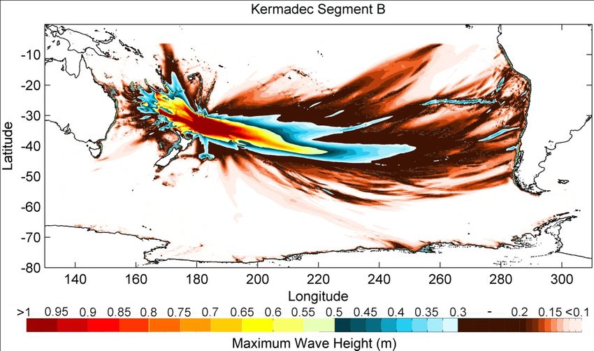
warning in the lower latitudes of the Pacific, especially given that the models demonstrate there is a
risk to coastal Antarctic research stations. There is also a need for improved bathymetric data and
for improved communications between relevant authorities and Antarctic base personnel. So that, in
the event of tsunami approaching on coastal Antarctica, personnel can benefit from an early warning
system that is accurate and effective. This preliminary study shows that further work is warranted
and that there is a need for competent authorities to actively participant in this work.

Background

Tsunamis may be generated by a number of different mechanisms; submarine landslide, bollide
impact, volcanic events and tectonic uplift of the seafloor. The common component leading to
tsunami formation is bulk water displacement occurring within a relatively short time frame. In this
report, tectonic deformation of the sea floor is the only source considered as it is the most frequent
cause of large tsunamis. Seafloor deformation producing tsunami is dominantly caused by the
displacement on a fault interface at converging plate boundaries, associated with subduction zones.
The subduction zones containing tsunami sources in this study are all situated along the Pacific Plate
boundary, they are the South American, Aleutian, Kermadec and Puysegur subduction zones.

Since the Ross Sea Region, West Antarctica and the Antarctic Peninsula all effectively open to the
Pacific Ocean, they are each potentially vulnerable to a large range of sources. There is thereby a
need to model a variety of sources to try and identify what orientations of subduction segments will
direct the generated tsunami wave at coastal regions in the Antarctic which currently support
personnel and/or infrastructure. Therefore, the focus of this project was primarily the Peninsula
Region (figure 1) and the Ross Sea Region (figure 2).

                                                  2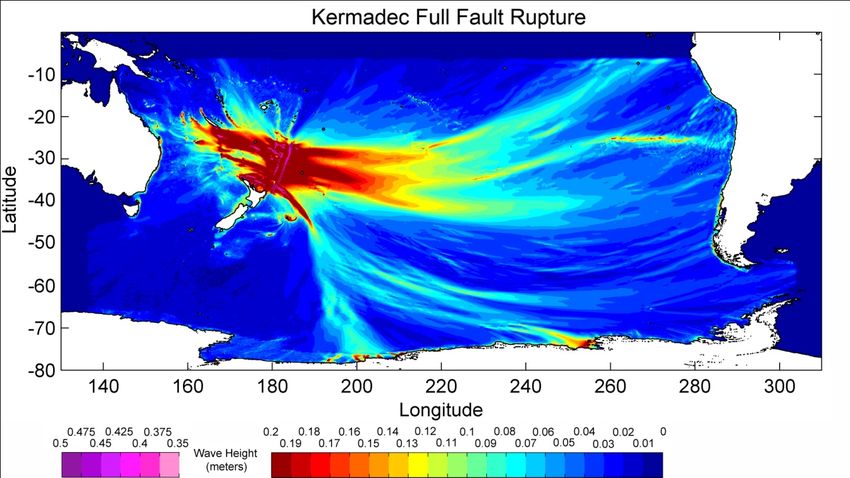
Figure 1: Antarctic research facilities in the Antarctic Peninsula. (Please note the map names are not from the
CGA and they are not an endorsement of COMNAP in any way). Not all facilities are shown, some stations of
high elevations or close proximity to already marked facilities have been left off this map.

Figure 2: Antarctic research facilities of the Ross Sea Region. (Please note the map names are not from the CGA
and they are not an endorsement of COMNAP in any way). Not all facilities are shown. This map also shows
locations of tidal gauges.

                                                       3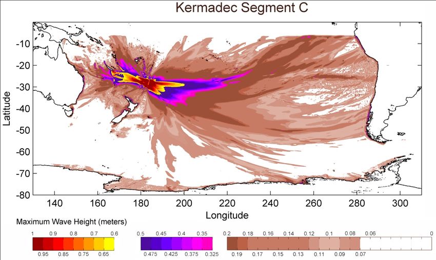
There are many factors which have contributed to the fact that, in the past, the Antarctic region has
literally been “left off the map” when it comes to tsunami modelling and tsunami hazard prediction.
Current tsunami modelling, by organisations such as NOAA, is usually area specific, meaning that
often such modelling rightfully focuses on areas of high coastal populations and cuts out areas of low
or no population (see Satake 2007, as an example). There is a need to be selective in order to be
efficient with respect to tsunami hazard evaluation. The computational time required by modelling
software can mean that Antarctica is excluded from models which take time to process tsunami
wave propogation to far‐reaching places from the tsunami source. The larger models cover larger
areas and hence require large bathymetry files that will affect the processing speed. Also, a desire
to have higher resolution images of an area of interest, has led to cropping of the full model tsunami
map. These factors have meant that Antarctica has, in the past, not been included in tsunami
modelling.

For “real” events, tsunami detection via buoys is the prominent method of active detection. The
tsunami buoy coverage for the Antarctic coastal region, however, is virtually non‐existent (figure 3).
Even buoys in the South Pacific are somewhat scarce and this limits the information available for
communication of real‐time tsunami threats to coastal Antarctic stations.

Figure 3: Map of the Pacific Ocean Region showing locations of network of tsunami detection buoys and also, around the Antarctic, the
location of tidal gauges. Deep Ocean Assessment and Reporting of Tsunami buoys (DART) is used here are a general label to cover the
closely related tsunami buoys DART, DART II and Science Applications International Corporation (SAIC) tsunami buoys (STB’s). ESR BPR’s
and Tidal gauges on this map were primarily used by the Antarctic Circumpolar Current Levels by Altimetry and Island Measurement
(ACCLAIM) programme but are monitored and presented at the ESR website. See http://www.ngdc.noaa.gov/hazard/tide.shtml for more
tidal gauges around South America.

                                                                   4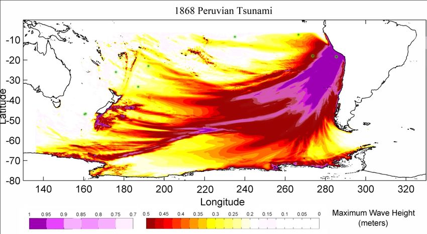
Methodology
Before models can be run, geometric parameters about the specific plate boundary need to be
known. These parameters are: fault length, fault width, epicentre, depth, strike, dip, rake or slip
angle and dislocation (of the fault plane in meters). Parameters used in the models originate from
journal articles from real earthquake events in the past, but in some cases, via interactive media
from recognised organisations such as the United States Geological Survey (USGS) or earthquake
data based used in the form of Google Earth KML files.

After obtaining the necessary parameters, a modelling area is defined and an equivalent and suitable
bathymetry file prepared. The suitable file in this instance was downloaded at 4 arc minute
resolution from the National Oceanic and Atmospheric Administration (NOAA) GEODAS Grid
Translator.

Bathymetry is important, as it largely controls the wave‐creating refractions, reflections, wave‐
guiding and dispersion effects. The reason the sea floor can produce these effects is because the
tsunami propagates in the entire water column. Once the bathymetry is added, the COMCOT can
then run at a matching resolution of 4 arc minutes grid size and at an appropriate 2.5 second time
step resolution.

The COMCOT output files were then processed using Matlab. The images are available as Appendix 1
to this report and as a poster (which will be on view at the COMNAP AGM). The images and the
known locations of Antarctic coastal infrastructure including research stations were then used to
determine relative risk from tsunami to those station and occupying personnel. For this preliminary
project, it was not possible to determine the effect that the presence of sea ice or ice shelves might
have on tsunamis.

 The images produced show maximum wave amplitude or equivalent sea surface elevation, obtained
over the lifetime of the modelling. The maximum amplitude images (Appendix figures A1 – A11)
have been processed up to three times each and the results have been combined using a simple
image overlay technique. The result is a maximum amplitude image that contains three scales of
tsunami wave height allowing more information to be displayed about the same event. Google
Earth image overlay was further used as a common ground for analysis to view tsunami images in
conjunction with tsunami buoy and base locations. In this report, the buoy locations have been
superimposed onto some figures for convenience otherwise the reader can refer to Figure 3 to view
the complete detection grid.

A series of these propagation images have been made into video files for further analysis.

Modelling Considerations
COMCOT is capable of modelling the entire lifespan of a tsunami from initial water column
displacement, through to the propagation of the tsunami across the ocean and also the inundation
of selected areas. Hence, is very suitable for the modelling required. However, modelling in this
report has not been done to the programmes highest potential as this would have been too timely,
therefore reasonable approximations have been made. Further work could be undertaken in this
manner if this initial project proves useful.

                                                  5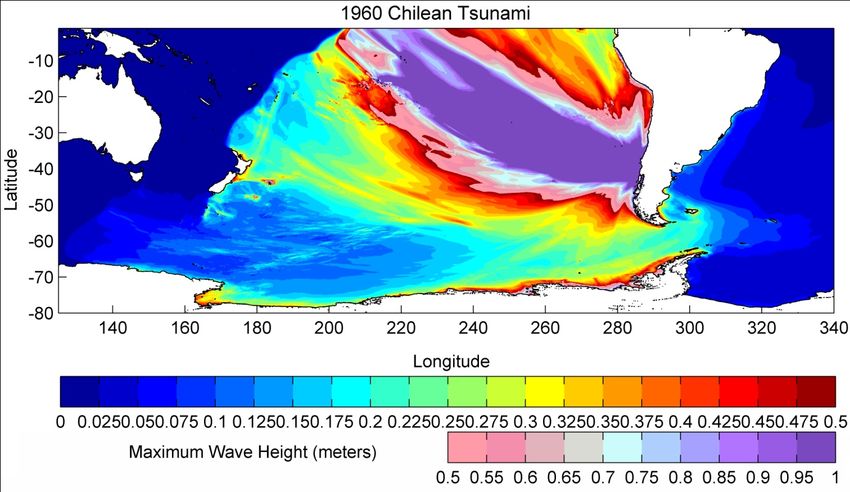
While linear shallow water equations have been used (figure 4), they cause the programme to
under‐evaluate tsunami wave height in regions where wavelength is large compared to the water
depth (coastal regions and perhaps continental shelf). The physical effect neglected here, is coastal
amplification or wave shoaling, and the rule of thumb is that the wave height can be approximately
double of that of the open ocean (Brigadier et al. 1948 on wind derived waves). There are models
that produce amplification factors that differ from those predicted by this rule, for example Satake
(1992) observed an amplification factor of three. It should be noted that approximation of the
amplification factor can be completely avoided if the non‐linear equations are used.

Secondly, inundation modelling was not attempted due to the complexity it would have added. To
model inundation, information regarding the Manning’s roughness coefficients for the Antarctic
regions, i.e. rock, ice and building coefficients would have been needed. The coastal region of
interest would then need to be mapped out and zoned by different coefficients before inundation is
run. Due to Antarctica’s high seasonality, the coefficients would vary considerably throughout the
year with the extent of the ice. These differences would mean that at least two Manning roughness
maps would be needed to be produced. Using two maps would require each tsunami scenario to be
run twice which is outside the time length of this project but could be undertaken in the next stage
of this project. Modelling has been run at mean sea level, therefore, tides need to be considered
when interpreting the results. Any risk analysis to the infrastructure should be done with high tide in
mind, since it is at high tide that the structure will be the most vulnerable.

The Linear Equations (Cartesian form):

                                                                  0                                     0

Equation 1.                                 Equation 2.                      Equation 3.
        where:
          is the water surface elevation.                             P = volume flux (West – East)
        f = Coriolis force                                            Q = volume flux (South - North)
        x,y and t are distance and time increments respectively       h = water depth

Figure 4: Equations used in the modelling software to produce the models.

Each model has been confined to an area, the boundaries of which behave differently depending on
the type of boundary selected. The characteristics of the boundary selected can be reflective,
absorbing or open. Two boundaries have been used in this report, the open boundary and the
sponge boundary. The open boundary allows the tsunami to pass straight through it and the sponge
boundary brings all physical properties to zero at the boundary. The sponge boundary is, physically,
the more robust or physically reliable option, but it reduces the modelling area. It is the sponge
boundary that is dominantly used in the models of this report.

                                                      6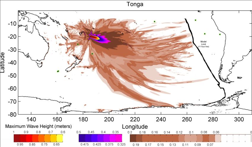
COMCOT evaluates volumes fluxes and water surface elevations at the most basic level in square
grids. It is in fact, an explicit, finite, “leap‐frog”, difference scheme that evaluates this. Auto
adjustment of the parent grid (the most basic layer) in COMCOT is an important choice for modelling
at polar latitudes. Deformation of the grid squares occurs near the Polar Regions as squares of
longitude and latitude in these regions are actually rectangular. Resizing of the COMCOT grid can be
done to counteract this effect by selecting the Parent Grid’s ID Number to 0.

Essentially the models ran in this project show where the tsunamis from distant tectonic sources are
directed to, in the vicinity of coastal Antarctica. What can be gained from the modelling is an
approximation of tsunami arrival time, an approximation of tsunami wave height and an indication
of the areas which are most or more often at risk or affected by a tsunami.

Results
Ten models were run using information from earthquake events from the following:

Kermadec ABC (Full Fault Rupture)                           Putsegur
Kermadec A                                                  Aleutian 1946
Kermadec B                                                  Chile 2010
Kermadec C                                                  Chile 1960
Tonga 1865                                                  Peru 1868
Table 1: The ten models that were run in the project.

The images produced after running the models can be found in Appendix 1 to this report. In all
cases, the models showed that there would be some increase in maximum wave height, although in
most cases that increase was relatively small (table 2).

Model                    The Ross Sea             The Antarctic Peninsula
Kermadec ABC             0.075                    0.075
Kermadec A               0.1                      0.1
Kermadec B               0.1                      0.1
Kermadec C               0.2                      0.2
Tonga 1865               0.04                     ‐‐not completed, ~ 0.1m as an
                                                  estimate
Puysegur                 < 0.05                   no expected effects
Aleutian 1946            0.1 to 0.2 of            0.5 to 1
                         tsunami wave
                         entering the Ross
                         Sea
Chile 2010               0.1                      0.3
Chile 1960               0.4 to 0.45              0.6 to 1+
Peru 1868                0.5 in general,          From 0.5 (East) and greater than 1
                         some areas up to         (West) and up to 2 in some “pockets”
                         1.5.
Table 2: Maximum expected wave heights in meters (without coastal amplification).

                                                        7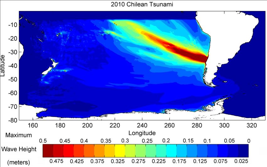
The results show, that there is a risk to coastal areas of the Ross Sea Region and to the Peninsula
Region from tsunami, especially from tsunami which originate from and are on the order of the
historical earthquake events of the Aleutian 1946, Chile 1960 and Peru 1868 (table 3). Since the
research stations and various facilities and infrastructure are not at the same height (above mean
sea level), a qualitative classification approach is used. The terms in the table have the meanings:
Minimal = less than 0.1m; Slight = 0.1m to 0.3m; Moderate = 0.3m to 0.5m; Concerning = greater
than 0.5m and can be greater than 1m.

       Model (see appendix)         The Ross Sea                 The Antarctic Peninsula
       Kermadec ABC                 Minimal                      Minimal
       Kermadec A                   Slight                       Slight
       Kermadec B                   Slight                       Slight
       Kermadec C                   Slight                       Slight
       Tonga 1865                   Minimal                      Slight‐Minimal
       Puysegur                     Minimal                      Minimal if anything
       Aleutian 1946                Slight                       Concerning
       Chile 2010                   Minimal                      Slight‐Moderate
       Chile 1960                   Moderate                     Concerning
       Peru 1868                    Moderate‐Concerning          Concerning
Table 3: Qualitative risk, based on the tsunami models run for the Ross Sea Region and the Peninsula Regions.

A full discussion of the results can be found in Appendix 2.

CONCLUSIONS
Of the ten models run for this project, the events of greatest concern to the Antarctic region are the
1960 Chilean tsunami, 1868 Peruvian tsunami and 1946 Aleutian tsunami. Models of lesser concern
include Puysegur, Kermadec and Tonga. Hence the source or zone of greatest concern in regards to
Antarctic coastal infrastructure appear to be from event originating from the Eastern Pacific
Subduction Zones. Since the Chilean coast has produced many large tsunami events historically and
it is quite close the Antarctic Peninsula this source is the greatest threat looked at in this report. But
of course the models are based on very specific past events and conditions will vary.

The most vulnerable coastal Antarctic research stations in the Antarctic Peninsula region are
Melchior, Actowski, Yelcho and San Martin as they sit at or below 5m. The Ross Sea Region’s lowest
research stations sit at 10m above sea level, so, are more protected from tsunami. However, large
tsunami events could potentially affect this region. The bases in the Ross Sea are largely naturally
sheltered from the brunt of tsunamis from the Pacific. Assessment of vulnerability is made via
human extrapolation of the linear tsunami modelling in this report to account for the shoaling
effects.

In terms of early detection, the tsunami buoys of greatest value, with respect to picking up large
amplitudes of the tsunami models run are 32401 (off the coast of Chile/Peru) for the Peruvian

                                                      8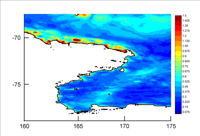
tsunami, 51406 (In the central Pacific) for the 1960 Chilean tsunami. All tsunami buoys can be
directly monitored by Antarctic‐based personal via the internet.

There are a host of other tsunami sources deserving attention of further modelling and research.
Obtaining maps for the roughness coefficients of the research stations would be valuable so that
inundation models could be run. Also the coefficients themselves may need to be revaluated as no
information was found on a value of propagation over (or under) an ice shelf.

This preliminary project has identified some key conclusions and comments for further
consideration, listed here in no particular order:

•   There is potential for some Antarctic research stations to be effected by tsunami under certain
    conditions mainly controlled by the tsunami source parameters and coastal amplification
    properties of coastal Antarctica. While the risk is general not high there is still a risk identified.
•   The location for placement of any new DART buoys or other monitoring instruments must be
    carefully selected, as there are “good” and “bad” choices when it comes to early warning for the
    Antarctic coast. Tsunami buoy location may wish to intercept the most immediate threat or it
    may wish to be suitably deployed in a location which picks up the best range of large tsunami
    signals for a single coastline of interest (perhaps in areas of Antarctica where there are large
    numbers of people based). Alternatively a well placed tsunami buoy could be selected to benefit
    Antarctic programs and other countries of the South Pacific. If the last option on placement was
    the desired outcome it should be noted that this may have a slight trade off in effectiveness for
    the Antarctic regions considered here.
•   The choice of monitoring device affects the quality of the data received, how often it is received
    and the cost associated with purchase, installation and maintenance.
•   There seems to be a lack of a common qualitative ways of communicating tsunami risk and there
    is a need to identify an effective communications plan and system.
•   The modelling program used in this report (COMCOT) had to be run on a setting such that the
    volume flux grid cells auto adjusted in the Polar Regions. It is important that any other tsunami
    modelling programs that attempt to model in the Polar Regions that they can in fact account for
    this. Also a suggestion to employ in further modelling would be to run the models at a higher
    resolution than 4 arc minute resolution, 1 and 2 minute data is available.
•   Bathymetric data is required to improve modelling capability.
•   No effects related to sea ice or ice shelf has been taken in to account when running this models.
•   No effect related to boundary conditions at the Polar Convergence have been taken into account
    and all tsunami sources modelled are north of the Polar convergence and therefore would cross
    this boundary.
•   Organisations with expertise in tsunami detection, modelling and research should work together
    with National Antarctic Programs on the next phase of this project.

                                                    9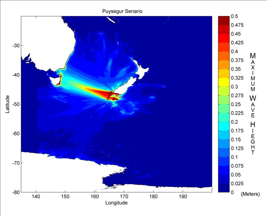
References
Brigadier R. Bagnold A. Barber N, Deacon G and Williams W. 1948 Coastal Waves. Nature vol 192
pp 682-684.

Fryer G. Watts P and Pratson L. 2004 Source of the great tsunami of 1 April 1946: a landslide in the
upper Aleutian forearc. Marine Geology. Vol 203 pp. 201-218.

Goff J. Walters R, Lamarche G, Wright I and Chaque-Goff C. Tsunami Overview Study 2005
Report for the Auckland regional council p4.

Hayes G.P. and Fulong K.P. 2010 Quantifying potential tsunami hazard in the Puysegur
subduction zone, south of New Zealand. Geophysics Journal International 183: pp1512-1524.

Hidayat D. Barker J. And Satake K. 1995 Modeling the Seismic Sources and Tsunami
Generation of the December 12, 1992 Flores Island, Indonesia, Earthquake. PAGEOPH 144:
Kanamori H. and Cipar J. 1974 Focal Process of the Great Chilean Earthquake May 22, 1960.
Physics of the Earth and Planetary Interiors 9: 128.

 Lopez A. and Okal E. 2006 A seismological reassessment of the source of the 1946 Aleutian
‘tsunami’ earthquake. Geophysics Journal International.

Okal E. 2007 South Sandwich: The Forgotten Subduction Zone and Tsunami Hazard in the
South Atlantic. Eos Trans. AGU, 89(53), Fall Meet. Suppl. Abstract OS51E-08.

Okal E. Borrero J. and Synolakis C. 2004 The earthquake and tsunami of 1865 November 17:
evidence for far-field tsunami hazard from Tonga. Geophysics Journal International 157: 168.

Okal E. and Hartnady C. 2009 The South Sandwich Island Earthquake of 27 June 1929:
Seismological Study and Inference on Tsunami Risk for the South Atlantic. South African
Journal of Geology 112.

Power W. and Gale N. 2011 Tsunami Forecasting and Monitoring in New Zealand. Pure and
Applied Geophysics 168:1131.

Satake K. 2005. Linear and Nonlinear Computations of the 1992 Nicaragua Earthquake
Tsunami. PAGEOPH vol 144 nos ¾ pgs 455 and 469 (whole paper is 455-470)
Satake K. 2007.Tsunamis Elsevier 4:17,2.

Satake K. and Kanamori H. 1990. Fault parameters and tsunami excitation of the May
23,1989, MacQuarie Ridge Earthquake. Geophysical Research Letters. 7:997.

Stirling M. McVerry G. and Berryman K. 2002 A New Seismic Hazard Model for New
Zealand. Bulletin of the Seismological Society of America. 92: 1883, pp1898-1899.

Tanioka Y. and Seno T. 2001 Detailed analysis of tsunami waveforms generated by the 1946
Aleutian tsunami earthquake. Natural Hazards and Earth System Sciences 1: pp171-175.

Thomas C. Livermore R. and Pollitz F. 2003 Motions of the Scotia Sea plates Geophysics
Journal International 155:785

                                                 10
Useful Websites:
Earth and Space Research (ESR)
http://www.esr.org/antarctic_tg_index.html
Bottom Pressure Recorder (BPR) info (unofficial)
http://www.oceans2025.org/PDFs/PDFs_of_powerpoints/Session_7B_Pete_Foden_POL.pdf
Global Disaster and Alert and Coordination System (GDACS)
http://www.gdacs.org/
Tropical Atmosphere Ocean (TAO) buoy dynamic height
http://tao.noaa.gov/ftp/OCRD/tao/taoweb/deliv/cache/data4329/README_dyn.txt)
National Data Buoy Center (NDBC)
http://www.ndbc.noaa.gov/obs.shtml
USGS rectangular earthquake grid search
http://earthquake.usgs.gov/earthquakes/eqarchives/epic/epic_rect.php
New Zealand’s tsunami gauges
http://www.geonet.org.nz/tsunami/
Antarctic Circumpolar Current Levels by Altimetry and Island Measurement (ACCLAIM)
http://www.psmsl.org/links/programmes/acclaim.info.php
https://www.comnap.aq/facilities
http://www.ioc-sealevelmonitoring.org/map.php
Intergovernmental Oceanographic Commission Tsunami Programme
International Tsunami Information Center. (ITIC)
http://itic.ioc-unesco.org/
United Nations Educational, Scientific and Cultural Organisation (UNESCO)
http://www.unesco.org/
Acknowledgments
Geological and Nuclear Sciences (GNS) Crown Research Institute, Wellington, New Zealand
Council of Managers of National Antarctic Programs (COMNAP)
University of Canterbury, Department of Geological Sciences
The University of Canterbury Summer Student Scholarship Scheme
11Appendix 1: Models
Figure A1: Maximum Wave Amplitude of the tsunami from a rupture along the entire Kermadec
subduction interface. Here the linear tsunami equations have been used.
Maximum wave height at DART tsunami buoy points:
55016 (0.2m), 54401(~0.2m), 51426 (~0.07m) and 32413 (0.07m)
Arrival times and tsunami descriptions:
A line of latitude originating at Cape Adare heading south defines the Ross Sea arrival point
from which the arrival time for all models is taken. For this model, the Ross Sea arrival time
is 6 hours and 10 minutes. Here the tsunami is a very small negative amplitude wave that
causes the sea to withdraw like a fast tide. The negative tsunami crest reaches the Antarctic
Peninsula by 9 hours 30 minutes at Cape Byrd then Adelaide Island at 10 hours 10 minutes.
A small positive tsunami crest follows the negative amplitude at the peninsula.
Fault Mechanism Overview: (supplied by GNS)
Strike Dip Rake Depth Dislocation Length Width Number
(range) of Faults
191.7- 4.0 - 90.0 3.97km- 2.2m 100km 50km 28
212.4 17.5 17.7km
Tsunami lifespan modelled: 15 hours.
12Figure A2: Maximum wave amplitude for a tsunami generated from the Kermadec A subduction segment
Maximum wave height at DART tsunami buoy points:
No tsunami waves are predicted by this model to be detected by any DART tsunami buoys.
Arrival times and tsunami descriptions:
Cape Adare arrival time: at 6 hours 10 minutes the first of a set of small tsunami waves arrive
that later wrap into the Ross Sea Region. The largest tsunamis are 0.1m in size,
Cape Byrd arrival time: 9 hours 50minutes the arrival of tsunami not greater than 0.1m which
is later followed by small tsunamis. The tsunami is directed at the Amundsen Sea and some
of that energy is swept off toward the Antarctic Peninsula.
Fault Mechanism Overview: (supplied by GNS)
Strike Dip Rake Depth Dislocation Length Width Number
(range) (range) (segment) (segment) of Faults
202.9 – 4.0 – 11.4 90.0 3.97km- 5.0 100km 50km 6
212.4 10.36km
Tsunami lifespan modelled: 15 hours.
13Figure A3: Maximum wave amplitude for a tsunami originating from a Kermadec B segment slip.
Maximum wave height at DART tsunami buoy points:
54401 (greater than 1m),
55016 (0.5-0.3m);
51426 (0.15m)
Arrival times and tsunami descriptions:
Ross Sea arrival time: 6 hour 10 at Cape Adare (0.1m wave)
Peninsula arrival time: Cape Byrd: 9 hours 40 minutes, Adelaide Is.: 10 hours 20 minutes
and at South Shetland Is: 10 hours 30 minutes. All tsunami waves are small and of about 0.1
meters in height.
Fault Mechanism Overview (supplied by GNS)
Strike Dip Rake Depth Dislocation Length Width Number
(range) (range) (range) (segment) (segment) of Faults
196.9 – 205 5.8 – 15.4 90.0 5.0 – 10.0m 100.0km 50.0km 11
15.1km
Tsunami lifespan modelled: 19 hours.
14Figure A4: Maximum wave amplitude for a tsunami generated from a slip on C segment of the Kermadec
trench.
Maximum wave height at DART tsunami buoy points:
55016 (0.9 to 0.85m), 54401 (0.65 to 0.6m) and to a lesser extent 51426(0.2m), 32413(0.18
to 0.12m), 32412 (0.18 to 0.12m) and 32401(0.09 to 0.07m).
Arrival Times and Tsunami Descriptions:
Ross Sea arrival time: 6 hours the draw-back arrives followed by a small 10cm tsunami half
an hour later.
Antarctic Peninsula receives the drawback at 10 hours and 10 minutes followed by a 10cm
tsunami at 11 hours at Cape Byrd.
Fault Mechanism Overview (Supplied by GNS)
Strike Dip Rake Depth Dislocation Length Width Number
(range) (range) (range) (segment) (segment) of Faults
191.7 – 9.55 – 90.0 6.51 – 8.0km 100km 50km 10
202.8 17.47 20.0km
Tsunami lifespan modelled: 20 hours.
15Figure A5: Maximum wave amplitude for the tsunami in 1865 originating offshore of Tonga.
Maximum wave height at DART tsunami buoy points:
51426 (0.5 m), 54401(0.1m) and 55016 (0.08m)
Arrival Times and Tsunami Descriptions:
Antarctic Peninsula arrival time: 10 hours 30 minutes (maximum between 11 and 12 hours)
Ross Sea arrival time: 6 hours 30 minutes the tidal retreat occurs, followed by a 10cm
tsunami at 7 hours and 40minutes and the maximum water height in the bay occurs between 8
and 9 hours)
Fault Mechanism Overview: (Model 1 in Okal et al. 2004)
Strike Dip Rake Depth Dislocation Length Width Number
of Faults
198.0 45.0 90.0 25.0 km 5.2 m 177.0 km 88.0 km 1
Tsunami lifespan modelled: 11 hours.
16Figure A6: Maximum wave amplitude for a tsunami originating from an oblique slip on the Puysegur
subduction zone
Maximum wave height at DART tsunami buoy points:
55015 (0.2m) and 55013 (0.35m)
Arrival times and tsunami descriptions:
The tsunami reaches Cape Adare at 3 hours and 20 minutes with an amplitude of 1cm. The
largest waves travelling into the Ross Sea during the 10 hours modelled do not exceed 5cm.
Antarctic Peninsula is not likely to receive any significant tsunami as the wave crest height
heading East is a mere 2.5cm.
Fault mechanism overview: (Hayes and Fulong 2010)
Strike Dip Rake Depth Dislocation Length Width Number
(range) (range) (range) of Faults
19.0 13.5 144.0 4.0 – 27.9 4.0m 134.6 – 17.68 – 5
km 318.1 km 32.28km
Tsunami lifespan modelled: 10 hours.
17Figure A7: Maximum wave amplitude of tsunami from the 2010 Chilean subduction interface slip.
Maximum wave height at DART tsunami buoy points:
32412 (0.2m)
Arrival times and tsunami descriptions:
Tidal drawback starts at the peninsula is at 1 hour for the South Shetland Islands and 50
minutes later at Adelaide Island and 2 hours 20minutes at 1. At 4hour 40minutes a tsunami
arrives at the Shetland Is rising to a maximum at 5-5.5 hours of 0.3m. The tsunami reaches
Adelaide Is. and Cape Byrd at 5 hour 30minutes. It enters the Ross Sea at 9 hours and 40
minutes after the initial fault rupture and is smaller than 10cm.
Fault Mechanism Overview: (GNS model)
Strike Dip Rake Depth Dislocation Length Width Number
of Faults
16.0 14.0 104.0 35.0 km 9.5m 420.0 km 100.0km 1
Tsunami lifespan modelled: 20 hours.
18Figure A8: Maximum wave amplitude for the 1960 Chilean tsunami.
Maximum wave height at DART tsunami buoy points:
51406 (1m >) to 32413(0.375 to 0.35m), 32412(0.375 to 0.35m), 32401 (0.5m), 51426(0.175
to 0.15m), 55016(0.175 to 0.15m) and 54401(0.225 to 0.2m)
Arrival Times and Tsunami Descriptions: Arrival times have at least a ⁄ 5 minute uncertainty.
At 3hours and 50minutes* the first tsunami wave reaches the South Shetland Islands. The
tsunami wraps around Adelaide Island and into Marguerite Bay at 4 hours 30minutes.
Maximum water height in the bay occurs between 5 hours 40 minutes and 6 hours 20 minutes
and ranges from 60cm up to 1m before considering shoaling effects. Nine hours after rupture
the tsunami reaches the Ross Sea, but the maximum amplitude arriving between 11 and 12
hours of approximately 0.4 meters. The first wave reaches Adelaide Island at 21 hours which
is promptly followed by two larger (0.5 meter) tsunami within the hour. No description is
given for the South Shetland Islands as they are within the sponge boundary for this model.
Fault mechanism overview: (Kanamori and Cipar 1974)
Strike Dip Rake Depth Dislocation Length Width Number
of Faults
10.0 10.0 80.0 30.0km 24.0m 800km 200.0km 1
Tsunami lifespan modelled: 13 hours.
19Figure A9: Maximum wave amplitude for the 1868 Peruvian tsunami.
Maximum wave height at DART tsunami buoy points:
32401 (2m +), 32412(0.55 to 0.6m) and 32413 (0.3 to 0.25m)
Arrival times and tsunami descriptions:
Antarctic Peninsula first arrival time: 7 hours 30minutes the tsunami hits the South Shetland
Islands. Ross Sea first arrival time: 12 hours 30minutes the first of a set of 25cm waves
arrives. See the nested grids (Figures 13 and 14 for further detail on the largest waves)
Fault Mechanism Overview:
Strike Dip Rake Depth Dislocation Length Width Number
(range of) (range) of Faults
305 to 316 20.0 90.0 20.0 km 15.0m 600km to 150km 2
300km
Tsunami lifespan modelled: 20 hours.
20Figure A10: A nested grid (still at 4 arc minute resolution) showing the maximum wave amplitude at the
Antarctic Peninsula for the 1868 Peruvian tsunami.
Figure A11: The nested grid (at the same resolution) showing the maximum wave amplitude at the Ross Sea
region for the 1868 Peruvian tsunami.
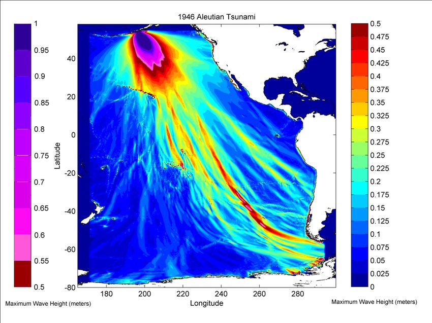
21Figure A12: The Maximum wave amplitude for the 1946 Aleutian tsunami with uplift of sediments
incorporated into the modelling parameters.
Maximum wave height at DART tsunami buoy points:
46408 (1m+) and 46403(0.5m) are buoys near the source offshore of the Aleutian trench (two
of many northern Pacific buoys that best measure this tsunami), 51406 (~0.5m), 32412
(~0.3m) and 51407(0.2m) which is just south of Hawaii.
Arrival times and tsunami descriptions:
This model produces a much larger secondary tsunami wave than the first tsunami wave.
The Ross Sea receives a tsunami not greater than 5 cm at 18 hours and 30 minutes. The
Antarctic Peninsula receives a 0.5m tsunami everywhere and in parts up to 1m. Arrival times
of the first wave are at 20hours 50 minutes at Adelaide Is. and 21 hours at Cape Byrd. South
Shetland Islands are affected by the sponge boundary and no reading can be given here.
Fault Mechanism Overview: (Tanioka Y. and Seno T. 2001)
Strike Dip Rake Depth Dislocation Length Width Number
of Faults
250.0 6.0 90.0 30.0km 27.5m 160.0km 30.0km 1
Tsunami lifespan modelled: 23 hours.
22Appendix 2: Full Discussion of Results
The Models
Models of historic tsunami or probable tsunami generating scenarios have been selected from
various sources to try and give a good coverage of the different directions that a tsunami
might realistically approach the Ross Sea or Antarctic Peninsula (the regions are affected
differently depending on the model).
Chilean Tsunami Models (See Figures A7 and A8)
Two of the tsunamis were modelled from the Chilean Subduction source were from large
energy tectonic ruptures; they were generated by the 9.5 magnitude earthquake in 1960 and
the 8.8 magnitude earthquake of Conception in 2010. The 1960’s tsunami is of great
historical significance as it affected a large portion of the Pacific as well as being devastating
locally. The Conception tsunami is a more recent event, smaller is size but relatively similar
in location. Notably there has been other large tsunami in history originating from the South
America subduction system and therefore more far-a-field tsunamis are reality from this
source in the future.
The 1960 model shows an effect in the Antarctic regions, forecasting for the Antarctic
Peninsula a maximum (linear) wave between 0.6 and 1m for most of the region with some
localities receiving waves in excess of 1m. For the tsunami the Ross Sea is expected to
receive about half a meter before amplification. The model of the 2010 tsunami shows that
the Antarctic region may only just be able to detect the tsunami and the Ross Sea may not
even be able to do that. The comparison between the 1960 and 2010 models illustrate a
massive variability of threat arising from sea floor deformations occurring on the Andes
subduction zone. Thus the exposure of Antarctic personnel to a dangerous tsunami from the
Chilean area needs to have the input of active monitoring so that a threat to the Antarctic
region from the Chilean Subduction interface can be distinguished. Greater coverage of
tsunami buoys in the low latitudes in the Pacific Ocean would be helpful so that this could
occur. If more buoys were present, then more reliable warnings could be given and
appropriate responses initiated.
23The 1946 Aleutian Tsunami - See Figure A12
The Aleutian tsunami was generated by an 8.1 magnitude earthquake, a relatively small
magnitude quake considering the tsunami large height that resulted. Local to the source at
Unimak Island, run-up is thought to have reached a colossal 42m (Lopez and Okal 2006) or
35m (USGS database) which is still very large. Theories as to why this happened include
submarine landslide models and uplift of sediments. This modelling in this report
incorporates the additional uplift of sediments which has been taken into account by
increasing the fault displacement (Tanioka and Seno 2001). Historically there have been
other significant tsunamis from the Aleutian Subduction zone of the Northern Pacific namely,
to the East the 1964 Alaskan tsunami and further west the 1957 Aleutian and 1952
Kamchatka tsunamis. Having one model run from this region provides a more global
understanding of the possible tsunami threats posed to the Antarctic region. When a tsunami
next occurs from a Northern Pacific subduction zone it will be well covered initially by
Northern Pacific tsunami buoys. By the time the tsunami enters the Southern Pacific the
tsunami’s characteristics will be better understood. In the Aleutian scenario modelled here the
Antarctic Peninsula is expecting waves of around 1m (before shoaling) while the Ross Sea
region does not receive any tsunami waves. The reason for this is the tsunami was highly
confined in wave front width as travelled toward the South (evident in Figure 15.)
Supporting evidence for a large tsunami from this model is provided by historic tsunami run-
up records (Fryer et al. 2004). Fryer et al. show that the peninsula received run-up heights in
the range of 1to 4 meters.
Limiting the modelling of the Aleutian tsunami is the sponge boundary found to have an
effect in the more eastern region of the peninsula. The result of the boundary is what looks
like tsunami waves between 10 and 20 cm in size. This edge region is misleading as
modelling here is subject to damping of actual wave heights expected.. The location of the
boundary could not be changed because of the restrictions placed on the largest bathymetry
file able to be downloaded. Such a boundary was required for the large travel times
associated with the scenario to reduce other unnatural effects. Large modelling times are a
follow on of large travel times and unfortunately modelling was cut short due to the model
not being pre-programmed to run long enough. The shortcoming results in the largest tsunami
wave stopping just short of the coast in the lowest latitudes. Even so, the model has proven
that the waves from this source stops can be expected at the Antarctic Peninsula although the
24full effects are unknown.
The (1868) Peruvian Tsunami See Figure A9
The Peruvian tsunami is generated from an 8.5 magnitude earthquake having a dislocation of
62.5% and a rupture area of 28.6% of that of the 1960 Chilean Tsunami. Yet the Peruvian
tsunami produces the largest tsunamis modelled here in this report for coastal Antarctica. The
reason is because the Peruvian segment is orientated such that tsunami originating from it are
directed at coastal Antarctic. That is, the source is efficient at preserving wave heights in
Antarctica’s direction.
This model has additional information in the form of nested grids (see Figures 13 and 14) to
provide added detail to the coastal regions of interest. Figure 14 reveals within the Ross Sea
region on the coast near the Mario Zuchelli base a larger tsunami height of 1.5 meters is
expected (three times larger than any other tsunami waves in the region). The Mario Zuchelli,
sits at 15m and therefore an impossible high amplification factor of 10 would be needed for
the station to be hit directly with a wave. Run up however is a slightly different to maximum
expected wave height as it depends on the volume and velocity of the driving waters behind
it. The Antarctic Peninsula can expect waves of larger than 1m (without coastal
amplification)
Kermadec Trench Tsunami Models ‐ See Figures A1, A2, A3 and A4
Modelling along of tsunami from the Kermadec subduction zone consisted of four different
rupture scenarios. All scenarios appear not to affect the Antarctic regions in any significant
way. No models produce waves with maximum wave heights greater than 20cm. Threat from
such a tsunami would likely only be from surging seaways perhaps unsuitable for small water
craft in coastal areas. The region that most consistently receives the larger tsunami waves
from this source is the unpopulated Amundsen Sea. This may need to be considered for any
potential projects planned for the future in the area. One of the models, Kermadec Segment A
produces a small far field tsunami; however, the 5m fault displacement parameter used is also
relatively small. If a larger displacement were to occur the direction that this wave travels
could have greater implications for the Antarctic Peninsula but not likely to the extent that the
South American events would.
25Kermadec segment B, produces the greatest tsunami for the whole of the Antarctic coastline
compared to the other Kermadec models. It is also this segment that has the largest predicted
fault displacement and here in lies the cause.
Puysegur Scenario See Figure A6
The energy from a rupture on the Puysegur subduction interface results in water surface
displacement that sends highly directional waves toward Australia and away from any areas
of interest of this study. Waves produced by this scenario are relatively small like the fault
displacement which the model is run from. If a larger displacement than four meters were to
occur then perhaps a small tsunami would be detected at the Ross Sea region. Tsunami buoys
55015 and 55013 are a proven necessity to provide warning for Australian coastal regions
and cities such as Hobart
Historically in the USGS database the 1989 quake having a depth of 10km and being of large
magnitude (8.3) would suggest that this southern extension of the Puysegur trench could be a
candidate for further tsunami modelling. The largest expected waves are very small and not
likely to exceed 5cm if they even made it the distance to the Ross Sea or Antarctic Peninsula.
Tonga ‐ See Figure A5
The Tongan model produces small tsunami waves for the peninsula and Ross Sea regions. In
comparison to the other smaller tsunamis of the West Pacific: Kermadec Segment A has a
similar displacement and produces a far smaller tsunami. The reason for the smaller tsunami
is because of the orientation of the fault rupture plain.
This model is stopped at 11 hours which is before the tsunami arrives at the peninsula. Figure
A5 and video analysis tend to suggest that any tsunami reaching the peninsula will be small.
The largest expected waves (without coastal amplification are)
Other Potential Tsunami Sources
The Scotia / South Sandwich plate boundary is an active subduction zone near the Antarctic
Peninsula that was not modelled in this report. Information on tsunamis generated from the
26region was not found but the region shows a reasonable seismicity using the USGS’s Google
earth files and it is an active plate system. One paper breaks down the plate boundary into six
segments using a statistical binning approach. In each of the geographical bins earthquakes
shallower than 60km and placed, then averaged to produce segments contains the averaged
parameters for strike dip and rake in the form of a double couple solution (Thomas et al.
2003). Other data in there paper could be reworked to produce some of the other parameters
needed (e.g. average depth) for tsunami modelling which could be used in conjunction with
reasonable assumptions on the dislocation to produce some tsunami models from the South
Sandwich subduction zone. Okal and Hartnady 2009 ran a model using the program Method
Of Splitting Tsunamis (MOST) from a magnitude 8.3 earthquake centred on the northwest
corner of the Scotia arc. The model was based on the earthquake in 1929 and the model
predicts 10 to 20cm waves (before coastal amplification) for the East coast of the Antarctic
Peninsula.
A model could not be run from the southern extension of the Kermadec subduction zone,
Hikurangi trench because of the uncertainty in the dislocation parameter. It is not really
known how much dislocation occurs on the fault plane when it ruptures (Stirling et al. 2002).
An additional tsunami hazard in the form of submarine landslide is also a point of concern for
the Hikurangi trench system (Goff et al. 2005). Earthquakes on the trench may generate a
tsunami from the faulting and trigger a submarine landslide the result of which being
additive.
The San Andreas Fault lies on the Pacific rim but was not looked at due to time constraints
but could be a possible source to model. A historic tsunami in 1992 generated by the strike
slip system produced significant local tsunami at Cape Mendocino but it is not expected to
have far-field consequences (González et al. NOAA Website)
There are a host of fault sources around the Antarctic region which may be able to generate a
local tsunami. A good example is the Macquarie Ridge earthquake 1989 for there is a record
of small tsunami waves landing in Australia (Satake and Kanamori 1990). Using the USGS’s
rectangular area tool a there are a series of magnitude 6 earthquakes on the South Pacific.
Any large rupture generating offshore of southern Chile would have a very short travel time
to the Antarctic Peninsula adding a level of danger as the chances of catching people unaware
27is much higher. Earthquakes of less than M 6.5 generally do not produce surface ruptures
(e.g., Wesnousky, 1986)
Comments and Other Considerations
The frequency of tsunami source events has not been considered in this report but is a
important factor that needs to be incorporated when considering the risk that a particular
scenario poses. Tsunamis generated less frequently should be given a lower risk weighting
than the same sized tsunami produced more frequently from a different source. The
frequency of event may influence the placement location of any tsunami buoys deployed in
the future. Location of tsunami buoys is a key issue, as poor, perhaps unlucky, placement can
yield a tsunami threat being down-played as the worst of the tsunami does not pass through
the buoy point.
Research stations may be above any expected tsunami level but that does not mean that the
whole of their operation is at or above the reported altitude. Many bases that are close to the
coast likely have boating access to the water hence at certain times personal may be below a
safe height or be on the water and critical marine infrastructure may also be at risk. Exposing
themselves like this may be daily routine and so providing adequate warnings to the Antarctic
coastal regions could save lives.
If possible it would be useful to compare the actual tsunami size with what the model height
is at known locations to see what kind of amplification factor we might expect.
When viewing the maximum amplitude files in detail there is a need to consider the
limitations of the modelling created from using the linear equations: coastal amplification,
wave path, wave breaking, and other effects. As the tsunami’s wavelength becomes
comparable to the water depth the bottom friction becomes important. The effect of using the
non linear equations to the wave motion is to give more control to the sea floor. Tsunami will
diffract into bays to a much greater extent due to the added friction. The bases of the
Antarctic Peninsula that are on sheltered side of an island or bay will experience more of an
effect. There is also the coastal amplification of the wave height and an expected delay in the
arrival times given.
All fault ruptures have been assumed to be instantaneous when in reality ruptures do have a
28propagation time. Thus some variation can be expected from the models presented in here
from this assumption.
Antarctica generally has a large time frame before a tsunami reaches it. The shortest (linear)
travel time of any tsunami modelled (regardless of its size) to the Peninsula is from the 1960
Chilean tsunami source having a travel time of around 3hours. Closer tsunami sources do
exist for the Antarctic Peninsula; the southern extension of the South America trench, the
plate boundaries associated with the Drake Passage as well as local submarine landslide and
volcanic sources.
Added dangers associated with tsunami in Polar Regions
Tsunamis in this report are perhaps not threatening to the majority of Antarctic facilities but,
tsunamis in Polar Regions are far more dangerous to the individual than in warmer climates.
A small tsunami may be strong or high enough to topple a person over. If a person is swept of
their feet in polar waters the consequences is far more life threatening than in the tropics.
Surges can drag people out to sea and often the Antarctic sea regions are edged with rock and
ice cliffs. Any damages occurring to Antarctic buildings or sea craft has greater implications
as repair or replacement is more limited in these distant and extreme environments, especially
for those coastal Antarctic stations that support winter-over personnel. Winter brings with it
an added vulnerability to people because of the darkness and the lower temperatures. Less
people will be exposed to tsunami threat in the winter as many coastal research stations only
operate in the summer season.
Environmental Concern: Ice Shelf Instability
The ice shelves and winter sea ice may be a useful tsunami buffer and damping mechanism.
A tsunami propagating under an ice shelf may cause the ice shelf to fracture under the
pressure of the positive crest. Furthermore the negative crest creates an air gap leading
potentially to sagging of the ice layer or if the change is rapid a suction effect may be
possible on the ice body. These added forces may damage or weaken the ice shelf and the
effects should be investigated further.
Tsunami Detection
For a tsunami warning system to be effective, a tsunami must first be detected and then the
information must be communicated quickly to all potentially affected regions. Seismic waves
29from earthquakes centred in submarine settings give early warnings to scientists that a
tsunami may have been generated. Coastal regions local to the source may not get any official
warning before a tsunami reaches them, as it depends on the whether a warning system is in
place and how far away the tsunami is. Distant coastal populations away from a tsunami
source should receive warning of a potential tsunami threat, as there is time to evaluate the
tsunami’s propagation if it is checked by suitable buoys. Another option to obtain information
on the tsunami’s likely path is by modelling (requires parameters of the generation
mechanism which have to be assumed or have become available through seismic analysis).
Parameters (fault, width and length) used in the tsunami modelling can be estimated using the
accumulation of aftershocks on the fault plane. Aftershocks, however, reveal the fault plane
over a period of time, making real time modelling by this method problematic. Quick
warnings may also be achieved one the magnitude of the earthquake is known by reviewing
pre-event constructed models; as practiced by Global Disaster Alert and Coordination System
GDACS.
30Appendix 3: Predicted Maximum Wave Heights at Buoys
Buoy 55016 54401 51426 32413 32412 32401 55015 55013 51406 46402 46403 51407
Figure 0.35- 0.20- 0.07- 0.07- 0.05- 0.05- 0.02- 0.02- 0.03- b b b
4.K 0.20 0.21 0.06 0.06 0.04 0.04 0.01 0.01 0.02
Figure 0.03- 0.07- 0.03- 0.01- 0.02- 0.01- 0.01- 0.01- 0.02- b b b
5.KA 0.04 0.08 0.04 0.02 0.03 0.02 0.02 0.02 0.03
Figure 0.65- 1.0+ - 0.13- < 0.1 0.14- 0.3- < 0.1 < 0.1 < 0.1 b b b
6.KB 0.6 0.95 0.12 0.13 0.2
Figure 0.85- 0.65- 0.20- 0.18- 0.18- 0.09- < 0.07 < 0.07 0.09- b b b
7.KC 0.80 0.60 0.19 0.12 0.12 0.07 0.08
Figure 0.07- 0.09- 0.5 – t t t < 0.06 < 0.06 < 0.06 b b b
8.To 0.06 0.08 0.475
Figure 0.025- 0.025 b t t t 0.2 0.35 t b b b
9.Pu 0 -0
Figure 0.05- 0.05- 0.075- 0.15- 0.175- 0.125 0.25-0 0.25-0 0.25- b b b
10.Ch 0.025 0.025 0.05 0.125 0.15 – 1.0 0.225
Figure 0.175- 0.225- 0.175- 0.375- 0.375- 0.5 0.025- 0.025- 1.0+ b b b
11.Ch 0.15 0.2 0.15 0.35 0.35 0 0 -0.95
Figure 0.2- 0.25- 0.25- 0.3- 0.6- >2.0* 0.15- 0.15- 0.15- b b b
12.Pe 0.175 0.225 0.225 0.25 0.55 0.125 0.125 0.125
Figure 0.05- 0.075- 0.1- 0.1- 0.275- 0.1- b b 0.375- 1.0+ - 0.475- 0.125-
15.Al 0.025 0.05 0.075 0.075 0.25 0.075 0.35 0.95 0.450 0.1
Table A1: Modelling predicted maximum wave heights (in meters) likely to be detected at the DART tsunami
buoys points in the open ocean (Locations of the buoys can be found in Figure 3). b= modelling boundary cuts
off buoy. t indicates that the modelling was stopped before tsunami (of any height) is able to reach the buoy
location. *additional range from and extra resolution ran which is not shown in any of the figures.
31You can also read