Movement patterns of white seabass Atractoscion nobilis tagged along the coast of Baja California, Mexico
←
→
Page content transcription
If your browser does not render page correctly, please read the page content below
Environ Biol Fish
https://doi.org/10.1007/s10641-021-01091-x

Movement patterns of white seabass Atractoscion nobilis
tagged along the coast of Baja California, Mexico
Scott A. Aalbers & Oscar Sosa-Nishizaki & Justin E.
Stopa & Chugey A. Sepulveda

Received: 31 October 2020 / Accepted: 6 April 2021
# The Author(s), under exclusive licence to Springer Nature B.V. 2021

Abstract This study outfitted wild-caught white                     15.2 ± 0.4 °C. Seasonal shifts in depth profiles to deeper
seabass (Atractoscion nobilis) with electronic data stor-           waters during the winter months were comparable with
age tags (DSTs) to evaluate subsequent movements of                 findings from previous tagging studies performed off
adult fish captured along Baja California, Mexico (BC).             California. Relatively high recapture rates reaffirm the
Cefas G5 DSTs were surgically implanted into 89 wild-               economic importance of this resource in both the U.S.
caught white seabass ranging in size from 66 to 152 cm              and Mexico, while tag recoveries within close proximity
TL between La Salina (32.11°N/116.90°W) and San                     to particular deployment sites suggest seasonal site fi-
Quintin (30.25°N/115.83°W), BC. Twenty-four tagged                  delity to specific geographic areas. White seabass move-
individuals (27%) were recaptured between April, 2010               ments between BC and California further support the
and May, 2017, following a mean time at liberty of                  transboundary nature of the stock and suggest that future
608 days (range = 18–1424 days) and a mean displace-                management would benefit from international fishery
ment of approximately 125 km (± 173 km; range = 3–                  policies.
720 km) between the point of release and recapture.
Tagged white seabass were recaptured between Santa                  Keywords Sciaenidae . Vertical movements . Depth
Rosalillíta, BC (28.66° N/114.27°W) and Monterey                    distribution . Electronic tagging
Bay, California (36.65°N/121.86°W), with four individ-
uals reported above the U.S-Mexico border. Collective-
ly, 8547 days of archived data revealed that white
                                                                    Introduction
seabass spent 95% of the time at depths
Environ Biol Fish
communities within the state of BC (Cartamil et al. that genetically distinct subpopulations exist both along
2011; Moreno-Báez et al. 2012; Romo-Curiel et al. Baja California Sur (BCS) as well as within the Gulf of
2015; Rubio-Cisneros et al. 2016). California, (Franklin 1997; Franklin et al. 2016). Re-
The vast majority of white seabass landed in Mexico gional differences in otolith microchemistry and growth
have traditionally been exported directly to the United rates of age 1 fish have also been identified, suggesting
States, with ex-vessel values ranging from $2.75–$3.64 some level of distinction between fish from the Southern
USD/kg between 2000 and 2006 (Escobedo-Olvera California Bight (SCB) and BCS (Romo-Curiel et al.
2009, Cartamil et al. 2011). More recently the export 2015; Romo-Curiel et al. 2016). Recent tagging work
market to the U.S. has grown considerably, with market has demonstrated transboundary movements between
prices nearly doubling over the past decade (Pers. southern California and BC (Aalbers & Sepulveda
Comm. D. Rudie). Market growth and steady demand 2015); however, it is unclear to what extent the resource
has led to an increase in directed fishing effort for white is shared between nations due to overall uncertainties in
seabass along the coast of BC and California, despite white seabass stock structure. It has long been suggested
declining trends in California landings and spawning that successful management of this transboundary re-
stock biomass since 2008 (Valero and Waterhouse source is dependent upon understanding fish move-
2016). ments and whether fish harvested along California and
Prior to 1982, a considerable proportion of the white Baja California Peninsula are part of one intermixing
seabass landed in California was harvested by 12 to 20 population (i.e. Panmixia) (Maxwell 1977; California
California-based gillnet vessels that fished along the Department of Fish and Wildlife 2002). The objectives
Baja California Peninsula during the fall and winter of this study were to assess white seabass movement
months (August–March; Skogsberg 1925; Vojkovich patterns and population connectivity through electronic
and Reed 1983). In some years, as much as 80% of the tagging of wild-caught individuals captured along the
annual U.S. commercial white seabass catch occurred in Baja California coastline and compare results with re-
Mexican waters, until foreign gillnet permits were re- cent tagging studies performed off southern California.
voked by Mexico in 1982 (Vojkovich and Reed 1983;
Escobedo-Olvera 2009). At the same time, Mexico be-
gan to explore the potential for harvesting white seabass
using small set and drift gillnets, pulled by hand Materials and methods
(Escobedo-Olvera 2009). The Mexican gillnet fishery
for white seabass grew quickly and is now an important Tagging procedure and sampling regime
source of seasonal income for fishers operating small
pangas, less than 10 m in length, out of fishing camps A total of 89 Cefas G5 and G5 long-life data storage tags
along the Baja California Peninsula (Escobedo-Olvera (DSTs; Cefas Technology Limited [CTL], Suffolk, UK)
2009; Cartamil et al. 2011; Cota-Nieto et al. 2018). were surgically implanted into the peritoneal cavity of
White seabass harvest along the Baja California Penin- wild-caught white seabass captured aboard 5-9 m
sula now predominantly occurs from May–September, pangas for hire along the BC coastline (Table 1). Cap-
with a peak in June (Escobedo-Olvera 2009), much of ture locations were dependent upon seasonal availability
which is still caught using hand-pulled gillnets near the within day-trip range of BC fishing communities be-
surface. However, a recent increase in the use of hy- tween La Salina (32.11°N/116.90°W) and San Quintin
draulic spools to haul larger gillnets has been noted (30.25°N/115.83°W), (Table 1, Fig. 1). Male and fe-
within several BC fishing communities, a trend that male white seabass, ranging in size from 66 to 152 cm
may continue to elevate fishing effort. TL (mean = 102 ± 24 cm) were opportunistically tagged
Despite a strong bi-national reliance on white seabass and released over five consecutive seasons from July 6,
stocks, population connectivity across their range re- 2009 to July 23, 2013. The majority of tagging occurred
mains uncertain. Based on range-wide genetic analyses, during the white seabass spawning season (Aalbers,
it has been proposed that white seabass harvested along 2008), with deployments during the months of June
the Pacific coast of California and BC are part of the (n = 31), July (n = 29) and August (n = 21), along with
same breeding population (Coykendall 2005; Ríos-Me- eight deployments in September. Specific procedures
dina, 2008), however; alternative hypotheses suggest for fish capture, tagging and sex determination wereEnviron Biol Fish
based around protocols further detailed in Aalbers and Data analysis
Sepulveda (2015).
Although this study was primarily focused on the All archived data sets were summarized at 2-min depth
movements of adult white seabass, a portion of the and 4-min temperature intervals to normalize time series
tagged females may have been immature considering among different sampling regimes (Aalbers and
that existing information on white seabass size of matu- Sepulveda 2015). Time series data generated from each
rity data remains uncertain (Maxwell 1977; Ragen tag recovery were formatted to Pacific Standard Time
1990). Based on preliminary findings from an inade- (PST) prior to generating summary statistics. Vertical
quate study that macroscopically examined gonads from rate of movement (VROM) was calculated for each set
a limited number (n = 3) of females between 70 and of recovered data (n = 20) as the absolute difference of
85 cm (Clark 1930), it was assumed that tagged females all subsequent 2-min depth records. The number of
greater than 79 cm TL were mature and that all males records of depth ≤ 5 m were calculated for each monthly
tagged in this study were mature. Thus, approximately period to identify seasonal differences in the frequency
10% of the females (n = 7) or unidentified individuals of occurrence of surface-oriented behavior. Mean daily
(n = 2) tagged in this study may have been immature, sea surface temperatures were derived from temperature
while three (13%) of the recaptured females (Environ Biol Fish
Table 1 White seabass data storage tag deployment and recovery specifics for 24 individuals recaptured between Santa Rosalillíta, BC and
Monterey, CA between May, 2010 and May, 2017
DST # TL Sex Deployment Deployment location Recapture Recapture location Days at Displacement
(cm) date (°N, °W) date (°N, °W) liberty (km)
A02168 124 F 6/20/2009 32.10, 116.90 6/28/2010 32.85, 117.28 373 91
A02165 132 F 6/20/2009 32.10, 116.90 9/11/2010 36.65, 121.86 448 680
A02132 91 NA 7/28/2009 31.22, 116.34 7/12/2010 31.82, 116.81 349 80
A02147 91 NA 7/28/2009 31.22, 116.34 1/31/2013 31.20, 116.36 1283 3
A02169 104 NA 7/29/2009 30.73, 116.05 4/25/2010 30.10, 115.83 270 73
A06053 84 F 8/9/2010 32.10, 116.90 5/15/2011 32.15, 116.91 279 5
A06055 130 F 8/9/2010 32.10, 116.90 4/27/2012 31.98, 116.80 627 17
A06048 130 NA 8/9/2010 32.10, 116.90 8/30/2013 31.57, 116.70 1117 62
A06052 109 F 8/12/2010 32.10, 116.90 7/9/2011 32.02, 116.88 331 9
A06046 119 F 8/12/2010 32.10, 116.90 9/25/2011 32.18, 116.92 409 9
A09239 104 F 8/29/2012 30.35, 115.88 8/19/2014 30.37, 115.96 720 7
A09240 112 M 9/21/2012 30.25, 115.83 8/10/2014 29.91, 115.76 688 38
A06056 66 M 9/21/2012 30.25, 115.83 5/3/2016 29.32, 115.12 1320 124
A09671 74 F 6/22/2013 31.39, 116.57 6/2/2014 31.41, 116.52 345 5
A09659 76 M 6/23/2013 31.40, 116.56 7/11/2013 31.52, 116.66 18 16
A09662 76 F 6/23/2013 31.37, 116.56 7/14/2015 32.55, 117.20 751 144
A06055b 81 F 6/23/2013 31.40, 116.56 7/5/2015 28.66, 114.27 742 377
A09667 91 M 6/23/2013 31.37, 116.57 6/6/2016 28.90, 114.47 1080 341
A09657 76 F 6/23/2013 31.39, 116.57 2/20/2015 31.02, 116.36 607 46
A03613 97 F 6/23/2013 31.40, 116.56 5/17/2017 31.11, 116.33 1424 39
A09979 88 F 7/19/2013 30.49, 116.10 7/17/2014 33.80, 118.41 363 427
A09976 81 M 7/19/2013 30.49, 116.10 7/19/2014 30.88, 116.27 365 46
A09975 86 NA 7/21/2013 30.49, 116.10 6/17/2014 28.66, 114.27 331 270
A09971 79 M 7/21/2013 30.49, 116.10 7/4/2014 31.20, 116.36 348 83
28.65°N, Long 114.21°W) and Monterey, California following recapture and two DSTs contained very little
(36.61°N, 121.87°W), following periods at liberty rang- data following redeployment with minimal remaining
ing from 18 to 1424 days (mean = 608 ± 381 days; Fig. battery life and were not used in subsequent analyses.
1). A 27% recapture rate was reported from local gill- Recovered DSTs with sufficient information provided
netters (n = 17), purse seiners (Sardineros; n = 2) and 8547 days of time series data consisting of 6.56 × 10⁶
sportfishers (n = 1) operating proximal to prominent depth and 3.28 × 10⁶ temperature records at 2-min and
BC fishing communities, as well as California-based 4-min resolution, respectively. Depth and temperature
gillnetters (n = 1), spearfishers (n = 1), hook-and-line records from at least one tagged individual were avail-
commercial (n = 1) and recreational fishers (n = 1). With able over a 6-year time period spanning from June 20,
the exception of one tag recovery in January and one in 2009 through June 17, 2015, with the exception a 66-
February, all additional recaptures occurred between day gap between June 23 and August 29, 2012 (Fig. 2a
late April and September. Complete time-series records and b).
from ten DSTs were directly downloaded at the PIER
lab upon recovery. Another ten DSTs were retrieved Horizontal movements
after the battery expired, but CTL engineers were able
to recover time series data for the active battery life of Tagged white seabass were at liberty for a mean dura-
the tag. Two DSTs were lost by fishers/processors tion of 608 days (range = 18–1424 days), with a meanEnviron Biol Fish
120° W
Colonet
San Quintin
30° N
Canoas
Santa Rosalillíta
115° W Baja California Sur (BCS)
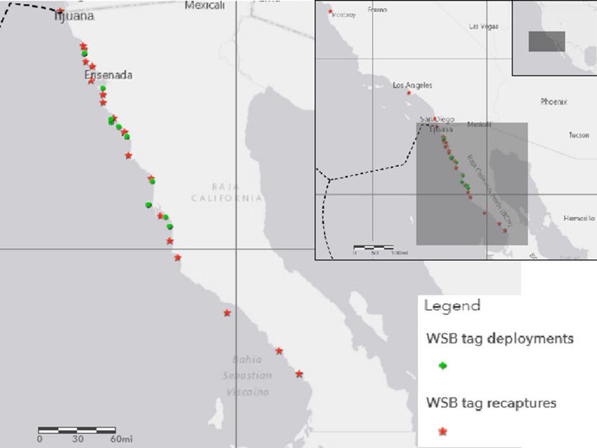
Fig. 1 Inset maps (shaded) displaying data storage tag deploy- indicates U.S. Mexico border and exclusive economic zone; solid
ments from July, 2009 through July, 2013 and recovery locations lines represent 5° latitude and longitude contours
from May, 2010 to May, 2017 for 24 white seabass. Dashed line
horizontal distance of 125 km (± 173 km) between the relationship between displacement distance and mean
point of tag deployment and recovery. Twelve individ- depth, with an increased mean depth for white seabass
uals were recovered within 50 km of their initial tagging that were recaptured more than 50 km from tag deploy-
site after a mean time at liberty of 591 (± 409 days). Of ment sites (mean = 23.5 ± 16.7 m) than for individuals
the tagged fish with a net displacement of more than recaptured close to initial tag deployments (mean =
50 km (n = 12), half of the recaptured individuals moved 13.0 ± 9.0 m).
southeast of their initial tagging location (138–163°
heading; mean 150°), while the other six individuals Vertical movements and temperature profiles
moved in a northwesterly direction (327–331° heading;
mean 329°). Four of the recaptured white seabass (17%) Although depths of up to 158 m were recorded, 95% of
were recovered above the U.S./Mexico border after the records were < 60 m (Fig. 3). Mean depth values
moving NW over a mean distance of 327 km. There ranged from 3.5 to 33.4 m between individuals with an
was no apparent trend in the direction of movement overall mean depth of 18.3 ± 12.9 m. Tagged fish
from specific tagging locations, irrespective of release reached a maximum monthly average (±SD) depth of
date. Additionally, there was no relationship between 31.1 ± 13.2 m in January and a minimum mean depth of
fish size and net displacement nor time at liberty and net 8.0 ± 5.9 m in July (Fig. 4). Surface-oriented move-
displacement (Table 1). However, there was an apparent ments were infrequent (Environ Biol Fish
a
0
2010 2011 2012 2013 2014 2015
10
20
30
Depth (m)
40
50
60
A02132 A02168 A06048 A06055 A09659 A09671 A09979
70 A02147 A02169 A06052 A06056 A09662 A09971 A09657
A02165 A06046 A06053 A09239 A09667 A09975
80
J A S O N D J FM A M J J A S O N D J FM A M J J A S O N D J FM A M J J A S O N D J FM A M J J A S O N D J FM A M J J A S O N D J FM A M J J
b
20
2010 2011 2012 2013 2014 2015
18
16
Temperature (°C)
14
12
A02132 A02168 A06048 A06055 A09659 A09671 A09979
10
A02147 A02169 A06052 A06056 A09662 A09971 A09657
A02165 A06046 A06053 A09239 A09667 A09975
8
J A S O N D J FM A M J J A S O N D J FM A M J J A S O N D J FM A M J J A S O N D J FM A M J J A S O N D J FM A M J J A S O N D J FM A M J J
Fig. 2 Mean daily (a.) depth and (b.) temperature profiles from 20 tagged white seabass that were at liberty from June, 2009 through June,
2015, with a 66-day gap in data between June 23 and August 29, 2012
during the winter months, whereas movements towards 15.7 m), temperature records did not reflect such a shift.
the surface were more common from June to September Mean temperature (14.6 ± 1.0 °C) during the winter
when tagged fish collectively spent 30% of the time months of 2009–10, 2013–14 and 2014–15 was slightly
within the upper 5 m of the water column. Despite higher than the collective mean temperature (mean =
considerable individual and inter-annual variation 14.1 ± 0.9 °C) from the winter months of 2010–11,
among white seabass tracks (Fig. 2a), significant differ- 2011–12 and 2012–13, when depth profiles were col-
ences in depth were apparent between the winter (De- lectively shallower (mean = 18.3 ± 5.7 m).
cember–February; mean = 29.8 ± 15.2 m) and summer Two smaller females (DST #A09662 & A09671)
months (June–August; mean = 9.2 ± 3.5 m; p val- exhibited a shallower depth distribution throughout the
ueEnviron Biol Fish
Fig. 3 Depth histogram by 5-m 0
bins based on 20 tagged white 5
seabass at liberty between June, 10
2009 and June, 2015
15
20
25
30
Depth (m)
35
40
45
50
55
60
65
70
75
0 5 10 15 20 25
Percent Occurence (%)
greater during the winter of 2014–15 (50.5 ± 14.5 m) discrete peaks at 3,4 and 5 cycles per day (Fig. 6).
when compared with mean depth during the winter of Longer-term periodicities (5–50 cycles per year), on
2013–14 (19.2 ± 14.7 m). the scale of 1 week to 2.5 months were highly variable
Depth probability plots constructed for each month and not persistent among all individuals.
further exhibited seasonal shifts in depth, with shallower Tagged individuals experienced water temperatures
distributions evident from April through October, tran- from 10.2 to 24.1 °C, with an overall mean of 15.2 ±
sitional periods during March and November, and 0.4 °C. Despite a relatively broad temperature tolerance,
deeper profiles from December through February tagged white seabass spent 73% of the time within a
(Figs. 5a-d). Depth probability plots also substantiated temperature range of 13–16 °C, with peak occurrence
heightened vertical rates of movement around dawn and around 14 °C (Fig. 7). Ninety-five percent of all tem-
dusk throughout all months of the year (Figs. 5a-d). perature records were between 12 and 19 °C, while 95%
Consistent daily (24 h) and semi-daily (12 h) peaks in of SSTs occurred between 13 and 19 °C. The mean SST
spectral density were evident from Fourier analyses of for all tag deployments was 16.5 ± 1.1 °C (range = 11.1–
depth data for multiple tracks (n = 19) along with 24.1 °C). Mean monthly temperatures reached a
0 18.0
5
17.0
10
16.0
Temperature (°C)
15
Depth (m)
20 15.0
25
14.0
30
13.0
35 Monthly-averaged Depth
Monthly-averaged Temperature
40 12.0
Jan Feb Mar Apr May Jun Jul Aug Sep Oct Nov Dec
Fig. 4 Mean (± 1 SD) monthly depth and temperature values summarized from 20 white seabass tagged along the coast of Baja CaliforniaEnviron Biol Fish
a January
10 10
0.04
20 20
0.03
30 30
40 0.03
40
Depth (m)
50 0.02 50
60 60
0.01
70 70
0.01
80 80
0.01
90 90
100 0.00 100
0 2 4 6 8 10 12 14 16 18 20 22 0 2 4 6 8 10 12
Hours in a day Cumulative Probability (%)
March
b 0.06
10 10
20 0.05 20
30 30
0.04
40 40
Depth (m)
50 50
0.03
60 60
0.02
70 70
80 80
0.01
90 90
100 0.00 100
0 2 4 6 8 10 12 14 16 18 20 22 0 2 4 6 8 10 12
Hours in a day Cumulative Probability (%)
Fig. 5 Joint probability of depth plots summarized into a 24-h period for the months of (a.) January, (b.) March, (c.) June, and (d.)
November consolidated from white seabass data storage tags deployed off the coast of Baja California
maximum of 16.5 °C in July, with a minimum of California, as inferred by Skogsberg (1939). Southward
13.3 °C in March (Fig. 4). movements across the U.S.-Mexico international border
were recently documented in a white seabass tagging
study conducted on wild-caught adults captured along
Discussion southern California (Aalbers and Sepulveda 2015), find-
ings that collectively validate some level of mixing
This electronic tagging study further substantiates white between white seabass off of California and BC. Verti-
seabass transboundary movements and provides the first cal movement patterns and temperature profiles of white
direct evidence of northward migrations from BC into seabass tagged in this study were consistent with tracksEnviron Biol Fish
c June
0.10
10 10
0.09
20 20
0.08
30 30
0.07
40 40
0.06
Depth (m)
50 50
0.05
60 60
0.04
70 0.03 70
80 0.02 80
90 0.01 90
100 0.00 100
0 2 4 6 8 10 12 14 16 18 20 22 0 2 4 6 8 10 12
Hours in a day Cumulative Probability (%)
November
d 0.06
10 10
20 0.05 20
30 30
0.04
40 40
Depth (m)
50 50
0.03
60 60
0.02
70 70
80 80
0.01
90 90
100 0.00 100
0 2 4 6 8 10 12 14 16 18 20 22 0 2 4 6 8 10 12
Hours in a day Cumulative Probability (%)
Fig. 5 (continued)
from fish tagged along California (Fig. 8; Aalbers and Stock structure and biological parameters
Sepulveda 2015), suggesting similar habitat utilization
and providing further support for an interrelated stock. Conflicting findings from genetic and otolith
However, a lack of tag recoveries reported south of microchemistry studies also warrant additional work to
Punta Rosalillíta, BC support the need for additional further assess the level of white seabass subpopulation
movement studies across BCS to further investigate structure (Coykendall 2005; Ríos-Medina, 2008; Frank-
the potential for a disjunct white seabass subpopulation lin 1997; Franklin et al. 2016; Romo-Curiel et al. 2016).
across the southern extent of their range. Although previous work has not revealed consistentEnviron Biol Fish
Fig. 6 Spectral analysis of white 2.5
seabass depth periodicities
displayed in cycles per day (CPD) 2.0
/cpd)
to indicate high-frequency diurnal
cycles for 19 sets of time series 1.5
2
data ranging in duration from 135
to 730 days upon application of a 1.0
Spectral Density (log10(m
fast Fourier transform algorithm
0.5
0.0
-0.5
-1.0
-1.5
-2.0
1.0 2.0 3.0 4.0 5.0 6.0
Cycles per day (CPD)
genetic differences across California and BC sampling conditions experienced by larval and juvenile white
regions (Coykendall 2005; Ríos-Medina, 2008), Frank- seabass reared along BCS may be different from indi-
lin (1997) concluded that the white seabass stock is viduals sampled off southern California and BC.
composed of a northern (Point Conception to central Portions of BCS, including Sebastian Viscaino
Baja California), southern (BCS), as well as a Sea of Bay and San Juanico Bay have been shown to sup-
Cortez component based on microsatellite DNA analy- port peak concentrations of larval white seabass
sis. More recently, Romo-Curiel et al. (2016) found during the months of May–August of 1950–1978,
ontogenetic differences in the isotopic composition of suggesting regionally important spawning areas
otolith growth rings, suggesting that the environmental (Moser et al. 1983). Peak abundance of 20–30 day-
Fig. 7 Summarized temperature 25
data by 1 degree C bins recovered
from 20 tagged white seabass at
liberty between June, 2009 and
June, 2015 20
Percent Occurence (%)
15
10
5
0
9 10 11 12 13 14 15 16 17 18 19 20 21 22
°
Temperature ( C)Environ Biol Fish
Fig. 8 Kernal density plot of 0.06
time-series data comparing S. California
collective depth profiles from 19 Baja California
white seabass tags recovered 0.05
following deployment off Baja
California and from 16 white
seabass tags recovered following 0.04
deployment off of southern
Probability (%)
California (Aalbers and
Sepulveda, 2015) 0.03
0.02
0.01
0
0 20 40 60 80 100
Depth (m)
old larvae have been identified in July along BCS, two archival tag returns from commercial sardine purse-
suggesting a later spawning peak than the May peak seine vessels (sardineros) confirm that purse-seining
in spawning reported off of southern California represented a notable source of white seabass fishing
(Aalbers 2008). Additional range-wide differences mortality. Whether captured as bycatch or directly
in the size structure (i.e. length frequency) and sea- targeted by purse seiners, it has been well documented
sonality of peak harvest have been identified that purse-seining for white seabass is both effective and
(Romo-Curiel et al. 2015), all potential indicators unsustainable, as this method rapidly led to overexploi-
of differentiated stocks or spawning areas. tation in the early fishery off California (Whitehead
1929). It was estimated that prior to 1925, purse seiners
Tag recoveries and other round haul nets landed more than 50% of the
total white seabass harvest off California (Croker 1937).
Ninety-two percent of tag recoveries occurred from late A steep reduction in California landings throughout the
April–September, confirming that peak harvest through- 1930s–40s is thought to have resulted from excessive
out the region occurs during the spring and summer targeting of white seabass spawning aggregations with
spawning season (Escobedo-Olvera 2009; Cota-Nieto purse-seine nets. Directed purse seine sets during the
et al. 2018). The seasonality of tag deployments and white seabass spawning season can be very effective
recoveries aligned with periods when California gillnet- and may contribute to a considerable level of under-
ters target white seabass near the surface (July–October) reported harvest.
(Skogsberg 1939). Similarly, gillnets are floated at the One of the white seabass tagged along BC was
surface along the BC coastline during the summer recaptured by a California gillnet fisher. A small fleet
months to target surface-oriented white seabass of approximately 20 gillnet vessels still actively target
(aboyados), whereas bottom set nets are generally a white seabass along California, however; gillnetting
more effective harvest method during the winter and practices were restricted in 1994 to waters outside of
early springtime (Escobedo-Olvera 2009). three miles from the coastline or one mile of the Channel
More than 70% of the recaptured white seabass in Islands (or > 128 m in depth; California Department of
this study were reported by small-scale gillnetters oper- Fish and Wildlife 2019). Harvest levels and participa-
ating along BC; however, tags were also recaptured by tion in the California gillnet fishery for white seabass
all other pertinent gear types used in the region. Al- have been in decline since 2010, with annual landings
though it was apparent that gillnets were the most prom- steadily declining below 100 metric tons from approx-
inent gear type used to harvest white seabass along BC, imately 30 active vessels in recent years (Valero andEnviron Biol Fish
Waterhouse 2016; California Department of Fish and individuals have been shown to reside within shallow
Wildlife 2019). coastal waters (Donohoe 1997) and it is likely that
Both U.S. and Mexican recreational fishers also overall movements are relatively limited during their
recaptured tagged white seabass in this study. White first few years of life (Maxwell 1977). Considering that
seabass are seasonally targeted by a large fleet of pri- existing information on white seabass size of maturity
vate, charter, and commercial passenger fishing vessels remains inconclusive (Clark 1930; Thomas 1968), it
that generate a high level of recreational fishing effort may be that some of the smaller females tagged in this
off California. Over the past two decades, southern study (e.g. DST #A09662, A09671) were immature and
California recreational fishing vessels have contributed did not exhibit broad horizontal or vertical movements.
to a significant proportion of the statewide white seabass Although it is unknown how far individuals may have
landings, occasionally exceeding annual commercial traveled during their time at liberty, migratory fish may
harvest levels (Aalbers et al. 2004; Valero and have shifted deeper along the continental shelf as oce-
Waterhouse 2016). Additionally, small pangas for hire anic conditions changed across latitudes. Additional
opportunistically target white seabass on hook-and-line deployments of geolocating archival tags along Califor-
from coastal towns throughout BC and BCS; however, nia and BC are underway, data which may better ad-
recreational catch and effort is not well documented and dress questions related to seasonal site fidelity, annual
considered to be low (Romo-Curiel et al. 2015). One migratory pathways and regional depth distributions
tagged white seabass was also recovered by a California (Aalbers and Sepulveda, unpublished data).
spearfisher, a more prominent method of take in recent
years from an increasing number of free divers that Vertical movements and temperature profiles
effectively target large individuals from seasonal
spawning aggregations across California and BC coastal Extensive time-series data accumulated over the six-
waters (Valero and Waterhouse 2016). year study period reflect many similarities to the depth
and temperature profiles reported for white seabass
Horizontal movements tagged off southern California (Aalbers and Sepulveda
2015), with significant increases in wintertime depth
A maximum displacement of 720 km between tag de- profiles documented in both studies. Inter-annual differ-
ployment and recovery sites suggests that white seabass ences in depth profiles were equivalent during the two-
have the potential to move extensively; however, the year period that these tagging studies overlapped, with
mean displacement distance of 125 km was weighted by increased mean depths during the 2009–10 winter
twelve individuals that were recaptured within 50 km of months relative to the winter period of 2010–11. For
their initial release site. One of the fish recaptured close this study, inter-annual depth shifts were collectively
to the tag deployment site was only at liberty for 18 days, greater in magnitude during the winter months of
yet the mean time at liberty for the other eleven individ- 2009–10, 2013–14 and 2014–15 (mean = 40.0 ±
uals was 639 ± 385 days (Range = 279–1283 days). 15.7 m) relative to wintertime depths from 2010 to 11,
Four of the individuals with net movementsEnviron Biol Fish
movement patterns of chinook salmon Onchorhynchus Management applications
tshawytscha were attributed to behavioral thermoregu-
lation in response to local thermal conditions, based on Historical white seabass catch statistics for Baja Califor-
temperature at depth measurements in the 8–12 °C range nia are difficult to aggregate for various reasons, how-
recorded by subsurface buoys off Monterey Bay, Cali- ever; the collection of additional information on spatial,
fornia (Hinke et al. 2005). Similarly, white seabass temporal and biological components of directed fishery
temperature profiles remained within a narrow range operations will continue to benefit future stock assess-
(13–16 °C) more than 70% of the time (Fig. 7), despite ments and sustainable management practices through-
significant seasonal changes in depth (Fig. 2a). Thus, out the region (Moreno-Báez et al. 2012; Valero and
white seabass movement patterns may be dependent Waterhouse 2016). California landings data have exhib-
upon regional temperature at depth profiles, suggesting ited dramatic fluctuations since the early 1900’s, with
that changing ocean conditions and temperature regimes several prominent peaks in catches during periods of
may influence white seabass migratory pathways. heavy exploitation followed by subsequent declines
Although fine-scale rates of vertical ascents and de- (Whitehead 1929; Skogsberg 1939; Thomas 1968;
scents were highly variable between tracks, FFT analy- Vojkovich and Reed 1983; Valero and Waterhouse
ses revealed diel patterns of vertical movement, with 2016). Findings from the first formal white seabass
spectral peaks identified at one and two cycles per day stock assessment indicate that spawning stock biomass
(Fig. 6). Diel movement patterns were also identified in has been in decline since 2007 and has been reduced to
adult white seabass tagged off California, along with less than 24% of the potential spawning stock biomass
comparable harmonic peaks at 3 and 4 cycles per day (Valero and Waterhouse 2016). Relatively high tag
that were attributed to vertical movements around the recovery rates documented along both California
mixed semi-diurnal tidal fluctuations and associated (24.3%; Aalbers and Sepulveda 2015) and Baja Califor-
shifts in thermocline depth typical for this region of nia (27.0%; this study) corroborate high rates of fishing
the eastern north Pacific (Cairns and LaFond 1966; mortality (F) first reported by Thomas (1968). Consis-
Aalbers and Sepulveda 2015). Diel and tidal periodicity tently high rates of electronic tag recoveries since 2009
identified in basking shark vertical movements was confirms that both U.S. and Mexican fishers rely heavily
attributed to cyclical foraging activity targeting concen- on this valuable international resource. When coupled
trations of prey that aggregated at daily and semi-daily with declining catch trends, findings support the need
intervals, particularly during periods of increased tidal for an updated stock assessment that incorporates rele-
amplitude and current intensity (Shepard et al. 2006). vant data sources from both U.S. and Mexico-based
Similarly, consistent vertical movement patterns have fishery operations. Extensive northerly and southerly
been recognized on diurnal scales in relation to foraging movements documented during tagging studies collec-
activity for a variety of other marine predatory species tively suggest a shared white seabass stock that season-
with diets consisting of small fishes and squid (Holland ally migrates between California and BC. Confirmation
et al. 1992; Lam et al. 2014; Afonso et al. 2014), of transboundary movements reinforces the need for
comparable to that of adult white seabass (Thomas collaboration between international government agen-
1968). White seabass movement patterns on a daily cies and the collective development of cohesive fishery
time scale may also be related to foraging activity management policies.
during periods when prey species tend to aggre-
gate or vertically migrate around dusk and dawn Acknowledgments We are grateful for continued support from
or following shifts in current direction surrounding the George T. Pfleger Foundation and the Offield Family Foun-
tidal changes. Although longer-term periodicities dation. We appreciate generous donations from the Catalina
Seabass Fund, Southern California Edison, the San Diego Fish
were not evident from FFT analyses, shifts in
and Wildlife Commission, the Avalon Tuna Club, Oakpower
depth observed across seasons align with reports Unlimited, and the Long Beach Neptunes. Gratitude to Tom
of higher white seabass catchability in bottom-set Pfleger and the Pfleger family, Chase and Calen Offield, John
gillnets during the winter months when fish are and Johnny Talsky, along with the legendary Paxson Offield, who
collectively supported and inspired this work. We greatly appre-
more closely associated with benthic habitats
ciate assistance and support from Kena Romo-Curiel, Sharon
(Escobedo-Olvera 2009, Pers. Comm. M. Herska, Omar Santana, Arturo ‘Masao’ Fajardo Yamamoto, Paul
McCorkle). Tutunjian, Tommy Fullam, Mike Wang, Mark Okihiro, VickiEnviron Biol Fish
Wintrode, Jennifer Thirkell, Jeanine Sepulveda and Kacy Lafferty gov/FileHandler.ashx?DocumentID=34195&inline.
along with cooperation from all fishers that assisted with tag Accessed 01 June 2020
deployments and reported tag recovery information. California Department of Fish and Wildlife (2019) White Seabass,
Atractoscion nobilis Enhanced Status Report.
Availability of data and material The data used to produce this https://marinespecies.wildlife.ca.gov/white-seabass/the-
manuscript has been uploaded to an online data repository and species. Accessed 23 March 2021
may be made available upon reasonable request to the correspond- Cartamil D, Santana O, Escobedo-Olvera M, Kacev D, Castillo-
ing author. Geniz J, Graham J, Rubin R, Sosa-Nishizaki O (2011) The
artisanal elasmobranch fishery of the Pacific coast of Baja
Funding Primary funding for this work was provided by the California, Mexico. Fish Res 108:393–403
George T. Pfleger Foundation and the Offield Family Foundation, Clark FN (1930) Size at maturity of the white Seabass (Cynoscion
with additional support from the Catalina Seabass Fund, Southern nobilis). Calif Fish Game 16:319–323
California Edison and the San Diego Fish and Wildlife Coffey DM, Carlisle AB, Hazen EL, Block BA (2017)
Commission. Oceanographic drivers of the vertical distribution of a highly
migratory, endothermic shark. Sci Rep 7:10434. https://doi.
Declarations org/10.1038/s41598-017-11059-6
CONAPESCA (Comision Nacional de Acaucultura y Pesca) (2017)
Animal Ethics Approval All live-fish capture and handling Anuario estadistico de acuacultura y pesca, Mexico, pp129.
procedures were approved by the Pfleger Institute of Environmen- https://www.gob.mx/conapesca/documentos/anuario-
tal Research Animal Handling and Ethics Committee (Protocol estadistico-de-acuacultura-y-pesca. Accessed 01 June 2020
#146–155.14-21). Cota-Nieto JJ, Erisman B, Aburto-Oropeza O, Moreno-Báez M,
Hinojosa-Arango G, Johnson AF (2018) Participatory man-
agement in small-scale coastal fishery-Punta Abreojos,
Conflict of interest All authors declare that there are no known Pacific coast of Baja California Sur, Mexico. Reg Stud Mar
conflicts of interest or competing financial interests that may have
Sci 18:68–79
influenced the material in this publication. All authors certify that
Coykendall DK (2005) Population structure and dynamics of
they have no affiliations with entities that have interest in the
white Seabass (Atractoscion nobilis) and the genetic effect
subject matter or financial interests in the material discussed in
of hatchery supplementation on the wild population.
this manuscript.
Dissertation University of California Davis
Croker RS (1937) The commercial fish catch of California for the
year 1935. Calif Dept Fish Game Fish Bull 49:73–75
Donohoe CJ (1997) Age, growth, distribution, and food habits of
recently settled white seabass, Atractoscion nobilis, off San
References Diego County, California. Fish Bull 95:709–721
Escobedo-Olvera MA (2009) Analisis biologico pesquero de la
pesqueria con red agallera de deriva en la peninsula de Baja
Aalbers SA, Stutzer GM, Drawbridge MA (2004) The effects of California durante el period 1999-2008. Dissertation Centro
catch-and-release angling on the growth and survival of de Investigacion Científica y de Educacion Superior de
juvenile white seabass captured on offset circle and j-type Ensenada (CICESE)
hooks. N Am J Fish Manage 24:793–800 Franklin MP (1997) An investigation into the population structure
Aalbers SA (2008) Seasonal, diel, and lunar spawning periodic- of white Seabass (Atractoscion nobilis), in California and
ities and associated sound production of white Seabass Mexican waters using microsatellite DNA analysis.
(Atractoscion nobilis). Fish Bull 106:143–151 Dissertation University of California Santa Barbara
Aalbers SA, Sepulveda CA (2015) Seasonal movement patterns Franklin MP, Chabot CL, Allen LG (2016) A baseline investiga-
and temperature profiles of adult white seabass (Atractoscion tion into the population structure of white Seabass,
nobilis) off California. Fish Bull 113:1–14 Atractoscion nobilis, in California and Mexican waters using
Afonso P, McGinty N, Graça G, Fontes J, Inácio M, Totland A, microsatellite DNA analysis. Bull South Calif Acad Sci
Menezes G (2014) Vertical migrations of a deep-sea fish and 115(2):126–135
its prey. PLoS One 9(5):e97884. https://doi.org/10.1371 Hinke JT, Foley DG, Wilson C, Waters GM (2005) Persistent
/journal.pone.0097884 habitat use by Chinook salmon Oncorhynchus tshawytscha
Andrzejaczek S, Gleiss AC, Jordan LKB, Pattiaratchi CB, Howey in the coastal ocean. Mar Ecol Prog Ser 304:207–220.
LA, Brooks EJ, Meekan MG (2018) Temperature and the https://doi.org/10.3354/meps304207
vertical movements of oceanic whitetip sharks, Holland KN, Brill RW, Chang RK, Sibert JR, Fournier DA (1992)
Carcharhinus longimanus. Sci Rep 8:8351. https://doi. Physiological and behavioural thermoregulation in bigeye
org/10.1038/s41598-018-26485-3 tuna (Thunnus obesus). Nature 358:410–412. https://doi.
Cairns JL, LaFond EO (1966) Periodic motions of the seasonal org/10.1038/358410a0
thermocline along the southern California coast. J Geophys Lam CH, Galuardi B, Lutcavage ME (2014) Movements and
Res 71:3903–3915 oceanographic associations of bigeye tuna (Thunnus obesus)
California Department of Fish and Game (2002) White seabass in the Northwest Atlantic. Can J Fish Aquat Sci 71: 1–15.
fishery management plan. https://nrm.dfg.ca. https://doi.org/10.1139/cjfas-2013-0511Environ Biol Fish
Maxwell WD (1977) Progress report of research on white seabass, Rubio-Cisneros NT, Aburto-Oropeza O, Ezcurra E (2016) Small-
Cynoscion nobilis. Calif Dept fish game, mar res admin rep scale fisheries of lagoon estuarine complexes in Northwest
(77-14), 14 p Mexico. Trop Conserv Sci 9:78–134
Moreno-Báez M, Cudney-Bueno R, Orr BJ, Shaw WW, Pfister T, Sibert JR, Lutcavage ME, Nielsen A, Brill RW, Wilson SG (2006)
Torre-Cosio J, Loaiza R, Rojo M (2012) Integrating the Interannual variation in large-scale movement of Atlantic
spatial and temporal dimensions of fishing activities for Bluefin tuna (Thunnus thynnus) determined from pop-up
management in the northern Gulf of California, Mexico. satellite archival tags. Can J Fish Aquat Sci 63:2154–2166
Ocean Coast, Manage 55:111–127 Shepard ELC, Ahmed MZ, Southall EJ, Witt MJ, Metcalfe JD,
Moser GH, Ambrose DA, Busby MS, Butler JL, Sandknop EM, Sims DW (2006) Diel and tidal rhythms in diving behaviour
Sumida BY, Stevens EG (1983) Description of early stages of pelagic sharks identified by signal processing of archival
of white seabass, Atractoscion nobilis, with notes on distri- tagging data. Mar Ecol Prog Ser 328:205–213
bution. Calif Coop Ocean Fish Invest Rept 24:182–193 Skogsberg T (1925) Preliminary investigations of the purse seine
Ojeda-Ruiz MA, Marín-Monroy EA, Galindo-De la Cruz AA, industry of southern California: white Seabass. Calif Div Fish
Cota-Nieto JJ (2019) Analysis and management of multi- Game, Fish Bull 9:53–63
species fisheries: small-scale finfish fishery at Bahia Skogsberg T (1939) The fishes of the family Sciaenidae (croakers)
Magdalena- Almejas, Baja California Sur, Mexico. Ocean of California. Calif Div Fish Game, Fish Bull 54:1–62
Coast Manag 178:1–8. https://doi.org/10.1016/j.
Stutzer GM (2004) Effects of intraperitoneal implantion of ultra-
ocecoaman.2019.104857
sonic transmitters on the feeding activity, growth, tissue
Ragen T (1990) The estimation of theoretical population levels for
reaction, and survival of adult white Seabass (Atractoscion
natural populations. Dissertation University of California San
nobilis). Dissertation California State University San Marcos
Diego
Ríos-Medina K (2008) Analisis de diversidad y estructura genetica Thomas JC (1968) Management of the White Seabass Cynoscion
de la corvina blanca (Atractoscion nobilis) de las costas de la nobilis in California waters. Calif Dept Fish Game, Fish Bull
Peninsula de Baja California (Mexico) y California (EE.UU.) 142:1–33
como primera aproxamacion para evaluar el impacto de su Valero J, Waterhouse L (2016) California White Seabass Stock
programa de repoblacion. Dissertation Universidad Assessment in 2016
Autonoma De Baja California Vojkovich M, Reed R (1983) White Seabass Atractoscion nobilis
Romo-Curiel AE, Herzka SJ, Sosa-Nishizaki O, Sepulveda CA, in California-Mexican waters: status of the fishery. Calif
Aalbers SA (2015) Otolith-based growth estimates and in- Coop Ocean Fish Invest Rept 24:79–83
sights into population structure of white Seabass, Whitehead SS (1929) Analysis of boat catches of white sea bass
Atractoscion nobilis, off the Pacific coast of North (Cynoscion nobilis) at San Pedro, California. Calif Div Fish
America. Fish Res 161:374–383 Game Fish Bull 21:1–27
Romo-Curiel AE, Herzka SZ, Sepulveda CA, Perez-Brunius
Aalbers SA (2016) Rearing conditions and habitat use of Publisher’s note Springer Nature remains neutral with regard to
white seabass (Atractoscion nobilis) in the northeastern jurisdictional claims in published maps and institutional
Pacific based on otolith isotopic composition. Estuar Coast affiliations.
Shelf Sci 170:134–144You can also read