MULTI-PHYSICS TRANSIENT SIMULATIONS WITH TRIPOLI-4 R
←
→
Page content transcription
If your browser does not render page correctly, please read the page content below

EPJ Web of Conferences 247, 07019 (2021)                                                               https://doi.org/10.1051/epjconf/202124707019
PHYSOR2020

               MULTI-PHYSICS TRANSIENT SIMULATIONS WITH TRIPOLI-4 R

                                Margaux Faucher1 , Davide Mancusi1 , and Andrea Zoia1
                   1
                       Den-Service d’Etudes des Réacteurs et de Mathématiques Appliquées (SERMA),
                               CEA, Université Paris-Saclay, 91191 Gif-sur-Yvette, France.

                            margaux.faucher@cea.fr, davide.mancusi@cea.fr, andrea.zoia@cea.fr

                                                                  ABSTRACT

               In this work, we present the first dynamic calculations performed with the Monte Carlo
               neutron transport code TRIPOLI-4 R with thermal-hydraulics feedback. For this purpose,
               the Monte Carlo code was extended for multi-physics capabilities and coupled to the
               thermal-hydraulics subchannel code SUBCHANFLOW. As a test case for the verifica-
               tion of transient simulation capabilities, a 3x3-assembly mini-core benchmark based on
               the TMI-1 reactor is considered with a pin-by-pin description. Two reactivity excur-
               sion scenarios initiated by control-rod movement are simulated starting from a critical
               state and compared to analogous simulations performed using the Serpent 2 Monte-Carlo
               code. The time evolution of the neutron power, fuel temperature, coolant temperature
               and coolant density are analysed to assess the multi-physics capabilities of TRIPOLI-4.
               The stabilizing effects of thermal-hydraulics on the neutron power appear to be well taken
               into account. The computational requirements for massively parallel calculations are also
               discussed.
         KEYWORDS: Monte Carlo simulation, neutron transport, multi-physics, transients, dynamic

                                                           1. INTRODUCTION

         Multi-physics simulations of nuclear reactor cores involve the coupling of neutron transport to
         other disciplines, such as thermal-hydraulics or thermo-mechanics. So far, such problems have
         mostly been analyzed using deterministic neutron-transport codes [1–3]. In recent years, intensive
         research efforts have focused on multi-physics calculations with Monte Carlo neutron transport
         codes in view of constructing high-fidelity simulation tools for the simulation of reactivity-induced
         transients in PWRs [4–6]. The goal is to provide reference solutions for neutron transport with
         multi-physics feedbacks.

         In this context, that we have implemented an external coupling scheme between the Monte Carlo
         code TRIPOLI-4 R [7] and the thermal-hydraulics subchannel code SUBCHANFLOW [8]. The
         coupling was realized by developing a multi-physics interface for TRIPOLI-4, which makes it
         possible to perform criticality calculations with feedback [9] as well as time-dependent coupled
         calculations via the use of the kinetic transport methods that have been recently conceived in
         TRIPOLI-4 [10]. In this work, we present the TRIPOLI-4 multi-physics capabilities for the simu-
         lation of transients and we illustrate them with a few configurations that were benchmarked against
         similar Serpent 2 calculations [11].

  © The Authors, published by EDP Sciences. This is an open access article distributed under the terms of the Creative Commons Attribution License 4.0
  (http://creativecommons.org/licenses/by/4.0/).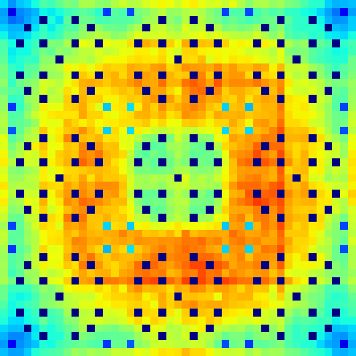
EPJ Web of Conferences 247, 07019 (2021)                                           https://doi.org/10.1051/epjconf/202124707019
PHYSOR2020

                                  2. TRIPOLI-4 MULTI-PHYSICS CAPABILITIES

         In order to be able to perform multi-physics calculations with TRIPOLI-4 and thermal-hydraulics,
         we have developed an external program, called “supervisor”, that drives a TRIPOLI-4 calculation
         step by step. The main role of the supervisor is to orchestrate data exchange between the coupled
         codes. The ICoCo API [12] from the SALOME platform serves as an interface to facilitate the
         coupling. The data exchanged between the two codes are represented in the form of fields on
         discretized meshes and are transferred in memory using the MEDCoupling library [13,14].

         TRIPOLI-4 scores the power distribution on a fuel-centered mesh. For SUBCHANFLOW, two
         meshes are defined: a fuel-centered mesh receives the power distribution from TRIPOLI-4, and
         a coolant-centered mesh is used for the resolution of the conservation equations. Note that the
         TRIPOLI-4 and SUBCHANFLOW meshes must have the same bounding box, but they do not
         need to superimpose exactly or to be numbered in the same way, as long as spatial interpolation
         is performed between them. The power distribution scored by TRIPOLI-4 is transferred to SUB-
         CHANFLOW using the interpolation tools provided by the MEDCoupling library. The subchannel
         code computes the updated properties of the fuel (temperatures) and the moderator (temperatures
         and densities), which are transferred back to TRIPOLI-4. Again, the MEDCoupling interpolation
         tools are used to transfer the SUBCHANFLOW results to the corresponding cells of the TRIPOLI-
         4 mesh. The TRIPOLI-4 material temperatures and densities are then updated; note that this
         requires the TRIPOLI-4 geometry to be discretized in such a way that each mesh cell corresponds
         to an individual volume. The temperature dependence of the cross sections is taken into account
         with stochastic interpolation in the Monte-Carlo code.

         Prior to a dynamic calculation, a criticality calculation with feedback must be performed to gen-
         erate the initial reactor state. During this phase, relaxation is imposed on the power distribution
         in order to achieve a smooth convergence. When the convergence has been reached, it is possible
         to store the fission sources in a file: the position, energy, direction and weight of each particle are
         written and can be used as the initial state for another calculation; in the case of dynamic calcula-
         tions, fission sources are converted into neutron and precursor sources for the dynamic phase by
         an additional power iteration [10]. For the time-dependent calculation, we formally apply the ex-
         plicit Euler discretized scheme for the system of coupled neutron transport and thermal-hydraulics
         equations.

         In general, the total CPU time is largely dominated by TRIPOLI-4 and parallelism is unavoidable.
         In a parallel calculation, we have chosen to have only one instance of SUBCHANFLOW for all the
         processors, so that the SUBCHANFLOW input is represented by the average power distribution
         calculated by all the parallel units. The rationale for this choice is that the thermal-hydraulics equa-
         tions are non-linear and the propagation of the statistical fluctuations through the coupling scheme
         is not straightforward. Averaging the power distribution over all the parallel units minimizes the
         fluctuations on the input to the thermal-hydraulics solver and the resulting bias.

         The TRIPOLI-4 parallelism scheme is the following. One parallel unit, the monitor, is in charge of
         orchestrating the other TRIPOLI-4 parallel units, of running the supervisor and SUBCHANFLOW.
         Another parallel unit (the scorer) is in charge of collecting the scores. The simulators are in charge
         of the TRIPOLI-4 simulation. When all simulators have completed a time step, the scorer collects
         the results and sends the averages to the monitor. The monitor sends the power distribution to

                                                            2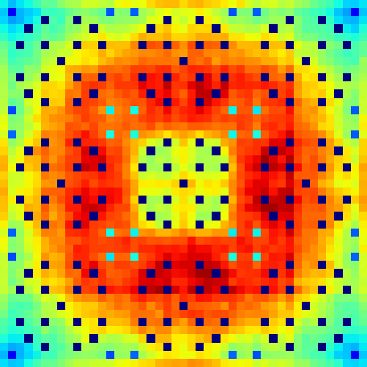
EPJ Web of Conferences 247, 07019 (2021)                                          https://doi.org/10.1051/epjconf/202124707019
PHYSOR2020

         SUBCHANFLOW, before finally launching the SUBCHANFLOW calculation. We emphasize
         the fact that the SUBCHANFLOW run can only start once all the simulators have completed the
         simulation of each time step.

                                                   3. TEST CASE

         The selected configuration, illustrated in Fig. 1, is a 3x3 mini-core based on the TMI-1 reactor [15].
         Each fuel assembly consists of 15x15 rods, made of 4.12% enriched UOX, and also contains four
         (Gd2 O3 +UO2 ) burnable poison pins. An instrumentation tube is located in the center of each
         assembly. Assemblies are surrounded by a reflector made of borated water and stainless steel (not
         shown in Fig. 1). The central assembly contains 16 extra control rods composed of a Ag-In-Cd core
         and Inconel cladding. The active length of 353.06 cm is divided into 30 axial slices. The coolant
         inlet temperature is set to 565 K, the outlet pressure is 15.51 MPa and the inlet mass flow rate is
         773.64 kg s−1 . The power of the system in stationary conditions is normalized to 140.94 MW. All
         the fuel and coolant compositions are individualized in the TRIPOLI-4 geometry, so as to be able
         to independently update their temperatures and densities.

          Figure 1: Radial view of the TMI-1 3x3 mini-core geometry implemented with ROOT for
          TRIPOLI-4. The central assembly contains 16 control rods (in blue). The burnable poison
                                        pins are represented in white.

         For the sake of simplifying the comparison with the published Serpent 2 calculations, we assume
         in this work that all the power is deposited in the fuel. In order to compute the fuel rod temperature,
         each axial slice of the fuel is divided into ten radial rings and the heat diffusion equation is solved
         with a finite-volume method. The fuel temperature returned by SCF is the the volume average over
         the radial nodes.

         The calculations have been run on the CEA Cobalt supercomputer at the TGCC (Très Grand Centre
         de Calcul, Bruyères-le-Châtel, France) with 1000 parallel units during 24 hours.

         Preliminary criticality calculations with feedback were performed to prepare the system on a criti-
         cal state, with the power being normalized to 140.94 MW. Control rods are full inserted in the core.

                                                           3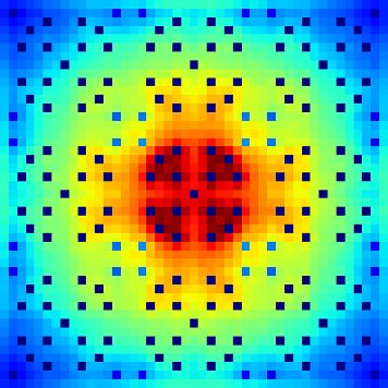
EPJ Web of Conferences 247, 07019 (2021)                                         https://doi.org/10.1051/epjconf/202124707019
PHYSOR2020

         With a boron concentration of 1305.5 ppm, the multiplication factor is keff = 1.00018 ± 8 × 10⁻⁵ ,
         showing that the system is close to a critical state. The resulting thermal-hydraulics fields were
         stored at the end of the calculation: fuel temperatures, coolant temperatures and coolant densi-
         ties, as well as the fission sources (position, energy, direction and weight of the fission neutrons
         for each one of the 1000 parallel units), to be used by the parallel units in charge of the dynamic
         calculations.

                                           4. TRANSIENT SIMULATIONS

         The purpose of the following transient simulations is to verify the TRIPOLI-4 multi-physics ca-
         pabilities. We therefore analyse the impact of thermal-hydraulics feedback on power excursions,
         and we also present the comparison between the TRIPOLI-4/SUBCHANFLOW results and the
         Serpent 2/SUBCHANFLOW results published in Ref. 11. Starting from the stored source (fission
         sources and thermal-hydraulics fields) mentioned above, the time evolution of the total power was
         followed over 5 s in 50 regularly spaced intervals by increments of ∆t = 0.1 s. As explained, at the
         end of each time interval, the neutron power is averaged over all the parallel units and transferred
         to SUBCHANFLOW, which then runs and solves the thermal-hydraulics equations for the time
         step. The next time step begins with the updated temperatures and densities. Population-control
         and variance-reduction methods specific to kinetic simulations are used, namely combing, forced
         decay and branchless collisions [16].

         In order to reduce correlations between the batches of the dynamic calculations, we have cho-
         sen to perform ten additional power iterations at the beginning of each batch, starting from the
         fission sources and thermal-hydraulics fields of the previous batch. SUBCHANFLOW is called
         with the new power distribution, and the compositions are updated. Thus, each batch of the dy-
         namic simulations begins with sensibly different fission sources, temperature and density fields,
         and correlations between the corresponding dynamic observables are considerably reduced.

         For the first scenario, the eight control rods are progressively extracted by 40 cm between t = 0.3 s
         and t = 1.3 s, which makes the system prompt supercritical with ∆ρ ≈ 1.3 $. The rod extraction
         is discretized in 10 steps. A second similar simulation was performed, with a less severe scenario,
         extracting the rods by 30 cm, which corresponds to a reactivity insertion of about ∆ρ ≈ 0.5 $.
         Each simulator completed seven full batches for the 30 cm scenario and four full batches for the
         40 cm scenario. The time evolution of the total power for both scenarios is shown in Fig. 2. The
         impact of the thermal-hydraulics feedback is clearly visible. First, the power is stable around
         140.94 MW between t = 0 s and 0.3 s, as expected. Then, the power increases up to 220 MW for
         the 30 cm scenario and up to 1100 MW for the 40 cm scenario. Finally, the thermal-hydraulics
         feedback mechanisms absorb most of the reactivity and drive the system towards an equilibrium
         configuration around 150 MW. The power peak is much sharper for the 40 cm scenario. The results
         obtained with Serpent 2/SUBCHANFLOW are also presented (the standard error was not available
         and is not shown). We find a very good agreement between the TRIPOLI-4/SUBCHANFLOW and
         the Serpent 2/SUBCHANFLOW results.

         The time evolution of the fuel temperature averaged over all the rods of the mini-core is also pre-
         sented in Fig. 2. As the reactivity increases, the average fuel temperature increases, then it remains
         stable after about 2 s. At the same time, the coolant temperature increases and the coolant density
         decreases as shown by Fig. 3. The final equilibrium state is characterized by higher temperatures

                                                           4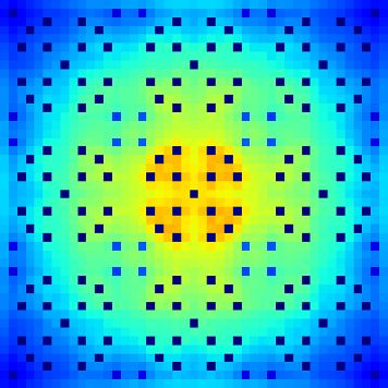
EPJ Web of Conferences 247, 07019 (2021)                                    https://doi.org/10.1051/epjconf/202124707019
PHYSOR2020

                    Figure 2: Simulation results of the TMI-1 3x3 mini-core computed with
           TRIPOLI-4/SUBCHANFLOW (red lines) and Serpent 2/SUBCHANFLOW (black lines),
          with control rods progressively extracted by 40 cm (top) and 30 cm (bottom). The reactivity
          insertion induced by the rods extraction is represented in green. Left: time evolution of the
         total power (in watts). Right: time evolution of the average fuel rod temperature (in kelvins).

            Figure 3: Average coolant temperature (in kelvins, left) and average coolant density (in
                              kg/m3 , right) for the same simulations as in Fig. 2.

                                                        5
EPJ Web of Conferences 247, 07019 (2021)                                             https://doi.org/10.1051/epjconf/202124707019
PHYSOR2020

         for the 40 cm scenario than for the 30 cm. There are some differences between the two coupling
         schemes, but the agreement is good overall; the maximum difference for the average fuel rod tem-
         perature is 10 K, in the peak power; the difference is below 1 K for the average coolant temperature
         and below 1 kg/m3 for the average coolant density. It is difficult to ascertain whether these discrep-
         ancies may be due to statistical fluctuations, since the temperature/density values at different times
         are strongly correlated.

         The increase with time in the fuel temperature for the 40 cm scenario is shown in Fig. 4 at a pin-cell
         level for two slices. Slice 3 is located close to the bottom of the mini-core, where the neutron flux
         actually rises because of the rod extraction; slice 10 is located above the rod extraction. For this
         reason, the increase is much larger for slice 3: the temperature increases up to 900 K at the center
         of the mini-core. For slice 10, the temperature mainly increases in the surrounding assemblies,
         since at this height the center of the mini-core contains the absorbant part of the control rods.

                 t = 1.3 s vs. t = 0.1 s            t = 2.1 s vs. t = 0.1 s                   t = 5 s vs. t = 0.1 s
                       0                             0                                       0
                900
                750   10                            10                                      10
                600   20                            20                                      20
                450
                300   30                            30                                      30
                150   40                            40                                      40
                0                                        0   10       20   30   40               0   10    20   30   40
                           0    10   20   30   40

                               Slice 3                            Slice 3                                 Slice 3
                225    0                             0                                       0
                200
                175   10                            10                                      10
                150
                125   20                            20                                      20
                100
                75    30                            30                                      30
                50
                25    40                            40                                      40
                0                                        0   10       20   30   40               0   10    20   30   40
                           0    10   20   30   40

                               Slice 10                       Slice 10                                Slice 10
               Figure 4: Radial maps of the increase in the fuel temperature (in kelvins), for the
           simulations in Figs. 2 and 3 (40 cm extraction), at three different times: t = 1.3 s, t = 2.1 s
         and t = 5 s, relative to t = 0.1 s. Top: temperature map for slice 3. Bottom: temperature map
                                                     for slice 10.

         It is worth stressing the fact that performing such massive parallel calculations is a real challenge.
         For the 40 cm extraction scenario, there are large variations among the parallel units; actually
         the calculation was slowed by one unit who suffered from severe positive fluctuations during the
         rod extraction. The median CPU time for the calculation of the time step between t = 1.2 s and
         t = 1.3 s is 130 s, while the slowest simulator took 6500 s. Half of the simulators were thus

                                                                  6
EPJ Web of Conferences 247, 07019 (2021) https://doi.org/10.1051/epjconf/202124707019
PHYSOR2020
inactive for almost two hours because of one single simulator. The large fluctuations in calculation
time probably reflect fluctuations in neutron population, which grow with the size of the neutron
population itself and are amplified by the branching nature of the fission process. In order to reduce
the total waiting time and increase the simulation efficiency, we have tried to enforce population
control on a tight grid during this time step (every 0.01 s), but no significant improvement was
observed. A tighter time grid may be required for this purpose.
Our coupling scheme exacerbates the negative impact of the fluctuations, because the thermal-
hydraulics solver is called only when all the simulators have completed their histories. One way
to improve the efficiency of the simulation would be to split the calculation into smaller, truly
independent replicas, with independent couplings to thermal-hydraulics. When all simulators of
the same packet have completed the time step, SUBCHANFLOW could be run without waiting for
the other packets, and at least these simulators could start the next time step. Therefore, we would
still be waiting for some packets, but fewer simulators would stay inactive during this time.
5. CONCLUSIONS
We have performed the first dynamic simulations with the coupling scheme between the Monte
Carlo neutron transport code TRIPOLI-4 and the thermal-hydraulics subchannel code SUBCHAN-
FLOW. For this purpose, we have considered a 3x3 mini-core based on the TMI-1 reactor. The
initial reactor state was calculated once with a criticality calculation including feedback. We reused
it for the two dynamic calculations.
We have studied two reactivity-insertion scenarios, with the control rods being extracted by respec-
tively 30 cm and 40 cm. For both scenarios, the feedback mechanisms make the power decrease
and ultimately reach a new equilibrium state. We compared our results to the published Serpent
2/SUBCHANFLOW results and generally found good agreement.
The simulation of the peak power is very challenging because of the large variations on the popula-
tion size. The 40 cm rod extraction especially induces a very large reactivity insertion (the system
becomes prompt supercritical), which leads to large fluctuations on the population size and thus
in CPU time among the parallel units. In particular, one unit was about 50 times slower than the
median. In order to mitigate the impact of fluctuations in CPU time among parallel units, the sim-
ulation could be split up in independent replicas. However, this solution is in tension with the need
to minimize the statistical fluctuations resulting from the Monte Carlo simulation.
ACKNOWLEDGEMENTS
This work was done within the McSAFE project which is receiving funding from the Euratom
research and training programme 2014-2018 under grant agreement No 755097. TRIPOLI-4 R is
a registered trademark of CEA. We wish to thank Electricité de France (EDF) for partial financial
support of the code TRIPOLI-4 R . We express our gratitude to D. Ferraro (KIT, Germany) for
providing the numerical data of the Serpent 2 calculations.
7EPJ Web of Conferences 247, 07019 (2021) https://doi.org/10.1051/epjconf/202124707019
PHYSOR2020
REFERENCES
[1] T. J. Downar et al. “PARCS: Purdue advanced reactor core simulator.” In Proceedings of the
PHYSOR 2002 conference. Seoul, Korea (2002).
[2] F. D’Auria et al. “The three-dimensional neutron kinetics coupled with thermal-hydraulics in
RBMK accident analysis.” Nuclear Engineering and Design, volume 238, pp. 1002 – 1025
(2008).
[3] A. M. Gomez-Torres et al. “DYNSUB: A high fidelity coupled code system for the evaluation
of local safety parameters – Part I: Development, implementation and verification.” Annals
of Nuclear Energy, volume 48, pp. 108 – 122 (2012).
[4] B. L. Sjenitzer and J. E. Hoogenboom. “Dynamic Monte Carlo Method for Nuclear Reactor
Kinetics Calculations.” Nuclear Science and Engineering, volume 175, pp. 94 – 107 (2013).
[5] M. Daeubler et al. “High-fidelity coupled Monte Carlo neutron transport and thermal-
hydraulic simulations using Serpent 2/SUBCHANFLOW.” Annals of Nuclear Energy, vol-
ume 83, pp. 352 – 375 (2015).
[6] R. Tuominen et al. “Coupling Serpent and Openfoam for Neutronics—CFD Multi-Physics
Calculations.” In Proceedings of the PHYSOR 2016 conference. Sun Valley, Idaho, USA
(2016).
[7] E. Brun et al. “TRIPOLI-4 R , CEA, EDF and AREVA reference Monte Carlo code.” Annals
of Nuclear Energy, volume 82, pp. 151 – 160 (2015).
[8] U. Imke and V. Sanchez. “Validation of the subchannel code SUBCHANFLOW using the
NUPEC PWR tests (PSBT).” Science and Technology of Nuclear Installations, volume 2012
(2012).
[9] M. Faucher et al. “Multi-physics simulations with TRIPOLI-4 R and Serpent 2: coupling neu-
tron transport with the sub-channel code SUBCHANFLOW.” In Proceedings of the ICAPP
2019 conference. Juan-les-Pins, France (2019).
[10] M. Faucher, D. Mancusi, and A. Zoia. “New kinetic simulation capabilities for TRIPOLI-4 R :
Methods and applications.” Annals of Nuclear Energy, volume 120, pp. 74 – 88 (2018).
[11] D. Ferraro et al. “Serpent/SUBCHANFLOW pin-by-pin coupled transient calculations for a
PWR minicore.” Annals of Nuclear Energy, volume 137, p. 107090 (2020).
[12] E. Deville and F. Perdu. “Documentation of the Interface for Code Coupling : ICoCo.”
Technical Report DEN/DANS/DM2S/STMF/LMES/RT/12-029/A, CEA, France (2012).
[13] V. Bergeaud and V. Lefebvre. “SALOME: a software integration platform for multi-physics,
pre-processing and visualization.” In Proceedings of the SNA + MC 2010 conference. Tokyo,
Japan (2010).
[14] SALOME (2019). URL https://www.salome-platform.org/.
[15] K. Ivanov et al. “Benchmark for uncertainty analysis in modeling (UAM) for design,
operation and safety analysis of LWRs. Volume I: Specification and Support Data for
the Neutronics Cases (Phase I), Version 2.1 (Final Specifications).” Technical Report
NEA/NSC/DOC(2013)7, OECD Nuclear Energy Agency, Paris, France (2013).
[16] M. Faucher, D. Mancusi, and A. Zoia. “Variance-reduction methods for Monte Carlo kinetic
simulations.” In Proceedings of the M&C 2019 conference. Portland, Oregon, USA (2019).
8You can also read