A novel approach to generate attractors with a high number of scrolls
←
→
Page content transcription
If your browser does not render page correctly, please read the page content below
A novel approach to generate attractors with a high number of
                                                                     scrolls
                                                                 J. L. Echenausı́a-Monroy1,2 and G. Huerta-Cuéllar0,1,2,3
                                          1
                                            Dynamical Systems Laboratory, CULagos, Universidad de Guadalajara, Centro Universitario de los
                                          Lagos, Enrique Dı́az de León 1144, Paseos de la Montaña, 47460, Lagos de Moreno, Jalisco, México.
                                          2
                                            Applied Mathematics Division, Instituto Potosino de Investigación Cientı́fica y Tecnológica, Camino
                                              a la Presa San José 2055, Col. Lomas 4ta. Sección, 78216, San Luis Potosı́, S. L. P., México.
                                             3
                                               Department of Physics and Earth Sciences, St.Marys University, SanAntonio, TX78228, USA.
                                                                  jose.echenausia@lagos.udg.mx1 , g.huerta@lagos.udg.mx0
arXiv:1904.03226v1 [nlin.CD] 5 Apr 2019

                                                                                            Abstract
                                                     In this paper, it is presented a novel method for increasing the number of scrolls in a hybrid
                                                 nonlinear switching system. Using the definition of the “Round to the Nearest Integer Function”,
                                                 as a generalization of a PWL function, which is capable of generating up to a thousand of scrolls.
                                                 An equation that characterizes the grown in the number of scrolls is calculated, which fits to the
                                                 behavior of the system measured by means of the coefficient of determination, denoted R2 , and
                                                 pronounced “R squared”. The proposed equation is based on obtaining as many scrolls as desired,
                                                 based on the control parameters of the linear operator of the system. The work here presented
                                                 provides a new approach for the generation and control of a high number of scrolls in a hybrid
                                                 system. The results are verified for all the scenarios that the equations covers.
                                                     Multiscroll attractors; High number of scrolls; Round Function; Unstable Dissipa-
                                                 tive Systems; Coefficient of Determination.

                                          1      Introduction
                                          The switched nonlinear systems are mostly associated to the generation of chaotic behaviors with
                                          the presence of multiple scrolls in their phase spaces [1, 2, 3]. The study of this kind of systems has
                                          presented a great interest in the last three decades of scientific development, due to the endless number
                                          of possible applications that these systems can have in different areas of science. The term multiscroll
                                          it is referred to the generation of an attractor that has, at least, three scrolls in its state space, unlike
                                          the dynamical systems of Lorenz [4] or Chua [5], which only have attractors of double-scroll. Suykens
                                          and Vanderwall [6], proposed this type of systems at the beginning of the 90’s, motivated by the idea
                                          of obtaining a richer dynamical system, referring to the number of scrolls, than the system of Chua,
                                          on which they were based.
                                               There are several approaches for obtaining systems with multiscrolls, which can be classified by
                                          considering their constructions as follows: i) adding break points to the function of Chua [7, 8], ii)
                                          using hysteresis functions [9, 10], iii) implementing functions of sinusoidal type and, iv) applying Piece-
                                          Wise Linear functions (PWL), [11, 12, 13, 14, 15]. By means of applying a PWL, an hybrid system is
                                          generated, which is characterized by the coexistence of continuos dynamics, such as the state variable
                                          of the numercial model, and logical decision making [16, 17]. The biggest handicap lies when the
                                          expected result entails obtaining a higher number of scrolls in the system.
                                               The generation of simple systems with a high number of scrolls is still an open problem, that’s
                                          why it is proposed an hybrid system based in the use of Unstable Dissipative Systems (UDS) [1, 2, 3]
                                          with the implementation of the Round to Nearest Integer Function as commutation law [18, 19], for
                                          the generation of attractors with a large number of scrolls, which can be controlled based on a growth
                                          equation dependent on the control parameters of the system, thus obtaining a system, numerically,
                                          easy to implement.
                                               This work is distributed as follows: the first section of the article contains a brief introduction to the
                                          problem where the scientific background is described. Throughout the second section, the basic con-
                                          cepts for designing UDS systems, as well as the mechanism for generating attractors with multiscrolls
                                          using PWL functions are described. The mathematical model used, as well as the description of the
                                          methodology implemented, are addressed in section number three. The results of the characterization
                                          of the model and the construction of the equation that governs the growth in the number of scrolls, are
                                          described in the fourth caption. The conclusions about the work are shown at the end of this paper.
                                              0 Corresponding   Author

                                                                                                 1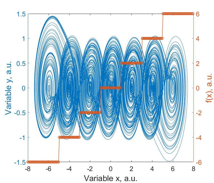
2 Theory
2.1 Unstable Dissipative Systems (UDS)
It is well known that the generation of attractors with multiple scrolls depends both, on the stability
of the generated equilibrium points, as well as on the type of the implemented switching function. It
is possible to analyze the stability of the equilibrium points through the theory of Unstable Dissipa-
tive Systems (UDS), which describes a variety of three-dimensional systems showing dissipative and
conservative components. The coexistence of both components causes the appearance of the so-called
attractors with multiscrolls.
As in previous works [3, 15, 19], consider a system of three coupled autonomous differential equa-
tions,
(1) Ẋ = AX+Bf(x),
where X = [x, y, z]T ∈ R3 , is the state vector, B = [b1 , b2 , b3 ]T ∈ R3 , is a constant position vector,
A = [ai,j ] ∈ R3×3 , is a constant matrix, and f(x) is a nonlinear function. The kind of behavior
exhibited by the system, is defined by the eigenvalues of matrix A, which can generate a great variety
of combinations and, therefore, the same diversity of behaviors.
Considering only the cases in which the system described by ec. (1) has saddle-node equilibrium
points, since they have both, stable and unstable varieties, it is possible to characterize the model in
the following way: i) a system it is considered as UDS I, if their equilibrium points are hyperbolic-
saddle-node, i.e., one eigenvalue is a negative real one, and the other two are complex conjugated with
positive real part, where the sum of the components must be less than zero. This last condition fulfills
the dissipative conditions of the system [2, 20]. ii) By the other side, a UDS II system it is defined as
those which has a real positive eigenvalue, and two complex conjugated with negative real part, where
the sum of its components it is also negative.
2.2 Multiscroll Attractors
If the linear operator of the system defined in ec. (1), fullfil all the conditions to be defined as a UDS
I, then it is possible to generate an attractor with multiple scrolls by means of the construction of a
commutation law, in this case, a PWL function. The purpose of the commutation law is control the
visit in the different equilibrium points of the system, being achieved by means of the coexistence of
a large number of one-spiral unstable trajectories. To illustrate such behavior [1, 3, 15], consider the
following linear operator:
0 1 0
(2) A= 0 0 1 ,
−0.6 −0.6 −0.6
which satisfiesP
the conditions that define a UDS I system, having eigenvalues equal to λ = [−0.8304, 0.3652±
1.2935 i] and λ = −0.1; this linear operator can be associated to a PWL function of three levels,
ec. (3). As can be seen in Figure 1(a), this conception of the function f (x) generates an attractor of
three scrolls with equally distributed trajectories and equidistant equilibrium points.
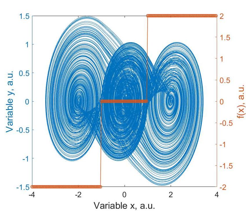
If the same linear operator as the one shown in ec. (2) is considered, and it is desired to obtain an
attractor with a higher number of scrolls, a new commutation law must be built in, taking special care
in obtaining equidistant equilibrium points, as well as the distribution of the trajectories. In order to
obtain as many scrolls as segments have been introduced to the switching function, i.e., be f (x) the
switching function presented in ec. (4), an attractor with seven scrolls in its phase space is obtaining,
Figure 1(b). This same exercise can be done to build in larger switching laws ec. (5), and therefore,
generate attractors with the same number of scrolls, Figure 1(c).
In general, the process to increase the number of scrolls in a system, is exemplified in the set of
equations ec. (3-5) in Table 2.2, the disadvantage lies when an attractor with many more scrolls must
be implemented, i.e. more than a hundred scrolls, which obviously implies a not so simple task to
address [21].
2
(a)                                            (b)

                          (c)                                            (d)

Figure 1: Attractors generated with the equations (a) ec. (2,3), (b) ec. (2,4), (c) ec. (2,5), (d) ec.
(2,6).

    The task of adding a higher number of equilibrium points to a system, in a simpler way, it is
possible through the implementation of a switching function as in [18, 19], where the results have been
validated for the generation of attractors with multiscrolls. As an example, the Round to the Nearest
Integer Function (RNIF) is implemented, ec. (6), which results in the attractor shown in Figure 1(d).

2.3    Multiscroll Generator System
The multiscroll generator system here studied, is similar to those studied in [3, 19, 22], which is
composed of three coupled differential equations, and implements a generalization of a PWL function
as an approach to obtain multiscroll attractors:

                                                ẋ = y,
                                                ẏ = z,
(7)                                 ż = −α1 x − α 2 y− α
                                                           3 z + α4 ,
                                                         x
                                         α4 = C1 g             ,
                                                        C2

whre the descriptor system to analyze is composed of three state variables x, y, z. The values α1,2,3
are control parameters of the system that can modify its dynamics, and α4 is the switching function
associated with the system. This work is focused on the operation region where the system responds

                                                   3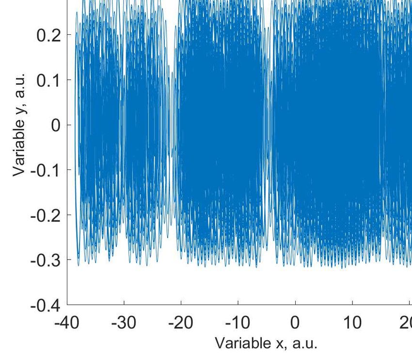
No. of scrolls PWL
−2, if x ≥ −1;
3 f (x) = 0, if − 1 < x < 1; (3)
2, if x ≤ 1.
−6, if x ≥ −5;
−4, if − 5 < x < −3;
−2, if − 3 < x < −1;
7 f (x) = 0, if − 1 < x < 1; (4)
2, if 1 < x < 3;
4, if 3 < x < 5;
6, if x ≤ 5.
−8, if x ≥ −7;
−6, if − 7 < x < −5;
−4, if − 5 < x < −3;
−2, if − 3 < x < −1;
9 f (x) = 0, if − 1 < x < 1; (5)
2, if 1 < x < 3;
4, if 3 < x < 5;
6, if 5 < x < 7;
8, if x ≤ 7.
h x i
N f (x) = 0.36 round . (6)
0.6
Table 1: PWL functions used for generate the attractors shown in Figure 1.
4to the configuration of eigenvalues defined as UDS I; so the system is studied under the premise that
all control parameters are equal, α = α1 = α2 = α3 .
Contemplating the previous statement, the behavior of the characteristic polynomial of the system,
λ3 +α(λ2 +λ+1) = 0, is analyzed under the modification for which the model responds to the definition
of a system cataloged as UDS I, resulting in a region of operation defined by 0 < α < 1.
In α4 , C1 and C2 are real constants associated with the control parameters of the system. The
function g(x) responds as the RNIF, in this case, of the state variable x. Because this definition of the
round function can be ambiguous for fractional values, the following consideration is adopted:
Up round, by taking ⌊x + 0.5⌋,
(8) g=
Down round, by taking⌈x − 0.5⌉.
The generalization of the nonlinear function, α4 , guarantees the generation of equidistant equi-
librium points [19], and the amplitude of the jumps between the different switching surfaces. This
conception is similar to those used in the set of equations described by ec. (3-5) (Table 2.2), and the
result is shown in Figure 1(d). The nonlinear function implemented in this system has a very simi-
lar operation to a PWL function, conceived in order to simplify the construction of many switching
surfaces as the control parameters allow.
3 Methodology and Results
As it has been demonstrated in previous works [18, 19, 22], the use of the nonlinear function α4 , ec.
(8), presents a dependence on the control parameters of the system, and on the integration time. This
is due that the function does not presents any type of limitation, either temporary or in the number of
switching surfaces to visit, so it is defined from −∞ to ∞. It is due to this, and the imperative need
to generate systems with a higher number of scrolls, that this work is focused on the characterization
of the system proposed by ec. (7), to obtain a system of easy numerical implementation, which is able
to generate as many scrolls as desired.
According to the considerations raised by the theory that describes the unstable dissipative systems,
it was established that the region where the analysis of the proposed model will be performed is defined
for values 0 < α < 1. Considering future electronic implementations, this control parameter will be
explored 0.05 ≤ α ≤ 0.95, and with a variation in the increment equal to ∆α = 0.05.
The system of equations, ec. (7), will be analyzed for each of the values in the control parameter
α, where the nonlinear function constants will be maintained as follows: C2 = 0.6, C1 = αC2 , which
guarantees the generation of equidistant equilibrium points. This system will be analyzed numerically
through the implementation of an integrator type RK4, and a time scale τ = 0.1. For each of the α
values analyzed, the integration time limit will be gradually increased, and the initial conditions of
the system will be randomly changed. For each combination in the parameters α − t, the number of
scrolls in the model is calculated. An equation describing the growth in the number of scrolls will be
approximated, generating a control law to generate attractors with a high number of scrolls.
In Figure 2, the obtained results from four different control parameters, α, and a sample of the
temporal values explored are shown. For example, consider α = 0.70 (green squares), the green
dotted line indicates the average of scrolls obtained (< N >), with the same marking color, both
the maximum (N Max) and minimum (N Min) values are shown. The results are analogous for all
the control parameters shown in the figure; turning the graph into a similar one to a box-plot. The
temporal spaces analyzed correspond to a value of 2σ , where σ is the x axis of the graph. The behavior
of the different curves presents the same growth trend, except for the value α = 0.95, where the increase
in the number of scrolls is slower, compared to the rest of the values.
Each of the analyzed control parameters yields similar results to those shown in Figure 2, which
can be summarized on the surface shown in FIG. 3a), where the increase in the number of average
scrolls is shown, N̄ =< N >, obtained for each of the control parameters with respect to time. Once
obtained the results, these can be analyzed to construct an equation that approximates the general
behavior of the system. In this case, the adjustment curve is constructed by linearizing the data [23],
resulting in the equation shown in ec. (9), such equation presents a dependency at two parameters,
the simulation time given to the system, t = 2σ , and the control parameter with which it is analyzed,
52500
α=0.20
α=0.45
2000 α=0.70
α=0.95
N Max
1500
N, a.u.
1000
N Min
500
0
14 16 18 20 22 24 26
Time, tσ, a.u.
Figure 2: Behavior of the number of scrolls generated, along time, for differents α values. The dotted
lines represents the average number of scrolls.
α. The behavior of this equation, under the same scenario as those proposed in the numerical analysis,
is shown in Figure 3(b).
ln(t)
β+
(9) 2
N̄ = e ,
where β is defined as in ec. (10), n∆α = α, responds to the value in the control parameter that is
analyzed, 1 ≤ n ≤ 19, and t is the time to be simulated in the system, C2 = 0.6.
3C2
(10) β = −∆α 28.2 + n 1 + .
n
500 500
450 450
2000 2000
400 400
1500 350 1500 350
, a.u.
, a.u.
300 300
1000 1000
250 250
500 500
200 200
0 150 0 150
2 26 2 26
1 100 1 100
0.75 2 22 0.75
2 19 50 50
0.5 Time, tσ, a.u. 2 18 0.5
Time, tσ, a.u. 0.25 0.25
2 14 0 Control parameter, α, a.u. 2 14 0 Control parameter, α, a.u.
(a) (b)
Figure 3: Surface of behavior in the average number of scrolls generated, along time, for all the α
values. (a) Obtained by means of the numerical time series analysis. (b) Obtained by means of
applying the ec. (9).
61
0.8
R2
0.6
R2 , a.u. 0.4
0.2
0
0 0.2 0.4 0.6 0.8 1
Control parameter, α, a.u.
Figure 4: Coefficient of determination (R2 ), between Figure 3(a) and Figure 3(b).
4 Discussion
Analyzing the behavior in the growth of the average scrolls, Figure 3, they seems very similar, but
it is not possible to trust in their apparent similarity; that’s why the coefficient of determination its
calculated for each of the curves experimentally obtained, against the theoretical curve that is generated
with the proposed equation. The coefficient of determination, denoted as R2 , and pronounced “R
squared”, is an statistic tool that determines the quality of a model to replicate results, and the
proportion of variation of the proposed results versus the original ones. The accuracy of the prediction
depends on the relationship between the variables to be analyzed. The coefficient of determination,
ec. (11), is defined as the square of the Pearson correlation coefficient; if the result is null, it is said
that the predicted variable does not have predictive capacity on the model; as this coefficient increases,
the prediction of the model turns out to be more accurate. The R2 values must to be between 0 and
1. For each α value, the same time values are analyzed, as in the numerical simulation, once these
data are obtained, the coefficient of determination that exists between the two information groups is
calculated, resulting in each of the points shown in Figure 4.
2
2 σxy
(11) R = ,
σx σy
where σxy is the covariance between the original data (x) and the proposed regression model (y), σx
is the standard deviation of the data and σy is the standard deviation of the model.
When its analyzed the behavior of the coefficient of determination, Figure 4, it is observed that
the equation fits in a very good way with the experimentally data obtained, where the average value
is R¯2 = 0.9440, red line Figure 4, confirming the prediction capability of ec. (9). The extreme values
presented in Figure 4, correspond to α = 0.05 and α = 0.95. This lack of prediction in the model can
be understood from the point of view of the distribution of the recurrence points from the Poincaré’s
section [15]. For very small α values, the disorder in the system is very high, so the visit to the different
domains is presented in a highly random way, being more difficult to estimate the number of switching
surfaces that will be visit. Similarly for values in the control parameter near to the threshold of the
UDS I region, where the system has gained a significant amount of order, so the visit to the different
switching surfaces is carried out with a probability that resembles to a Normal distribution, so the
prediction in such scenario, also becomes difficult.
70.4 5
0.3
0.2 0
Variable x, a.u.
Variable y, a.u.
0.1
0 -5
-0.1
-0.2 -10
-0.3
-0.4 -15
-15 -10 -5 0 5 0 2 4 6 8
Variable x, a.u. Time, t, a.u. ×104
(a) (b)
Figure 5: a) Attractor with N = 27 scrolls, and b) Time serie of the x variable, for the parameters
α = 0.5, and t = 70000 units.
4.1 Equation Validation
To demostrate the correct operation of the proposed equation, ec. (9), the following results are
presented, Table 4.1, that cover the three possible scenarios: i) when α and t are known values,
determine the number of scrolls to be obtained ec. (9), ii) when is desired to obtain an attractor of
N scrolls for a determined α value, determine the simulation time that takes the system to reach the
visit of the N switching surfaces ec. (13), and iii) when both values, N and t, are set parameters,
determine the α value that is required to obtain the desired attractor ec. (14).
Considering the first case proposed by ec. (9), suppose that the control parameter is known, as
well as the simulation time to be used, α = 0.5, t = 70000 u., and it is desired to know the number of
scrolls to be obtained, this to determine if the attractor is large enough for the purposes, or a higher
number of scrolls is required. With this information, it is possible to estimate the number of scrolls
that would be obtained by substituting in ec. (9), resulting an average number of scrolls N̄ = 35.8064.
According to the results of the equation, the system must present around of 36 scrolls in its phase
space, for the parameters α = 0.5 and t = 70000 units. If this scenario is simulated, the system
presents the dynamics shown in Figure. 5, where an attractor with 27 scrolls is obtained, which is not
so different from the value dessired.
In the same way as in the previous case, it is possible to perform the following exercise: an attractor
with a hundred of scrolls is desired, associated to a control parameter α = 0.35, so the simulation time
needed to obtain such attractor is the parameter to calculate. Substituting these values in ec. (13),
t̄ = 404470 u. is obtained. This amount of time may be considered as the minimum time that the system
needs to visit all the switching surfaces desired. If the system is simulated with these parameters, an
attractor with 108 scrolls is obtained, Figure. 6.
As a last proof of the right prediction performed by the equation that governs the number of scrolls
to be obtained, assume a simulation time t = 23000 u., and the desired number of scrolls is N = 13, so
the control parameter to be used is unknown. Substituting the information in ec. (14), n̄ = 19.1335 is
calculated, which is rounded to n̄ = 19, and corresponds to α = 0.95. Carring out the simultaion, the
system presents an attractor with only 5 scrolls. As mention before, the system is hard to predict in
this α value, because of the order that the dynamics in the system has gain. Considering this fact, the
simulation it is performed for the α previous value (α = 0.9), where the system exhibits an attractor
with 12 scrolls, Figure 7.
8Known Parameters Estimated Parameter
ln(t)
β+
2
α, t N̄ = e . (9)
N
2 ln
eβ
α, N t̄ = e . (13)
N 1
t, N n̄ = −(3C2 + 28.2) − ln . (14)
ln(t) ∆α
2
e
Table 2: Combinations of the equation for control the growth of the number of multiscrolls.
30
20
10
Variable x, a.u.
0
-10
-20
-30
-40
0 1 2 3 4 5
Time, t, a.u. ×105
(a) (b)
Figure 6: a) Attractor with N = 108 scrolls, and b) Time serie of the x variable, for the parameters
α = 0.35, and t = 404470 units.
90.4 6
0.3
4
0.2
Variable x, a.u.
Variable y, a.u.
0.1 2
0
0
-0.1
-0.2
-2
-0.3
-0.4 -4
-2 0 2 4 0 0.5 1 1.5 2 2.5
Variable x, a.u. Time, t, a.u. ×104
(a) (b)
Figure 7: a) Attractor with N = 12 scrolls, and b) Time serie of the x variable, for the parameters
α = 0.9, and t = 23000 units.
5 Conclusions
With this research work, a hybrid system of three differential equations that implements the Round
to the Nearest Integer Function, as a generalization of a PWL function, for obtaining systems with
multiscrolls based on UDS models, has been analyzed. Based on the implementation of the RNIF, a
characterization of the behavior of the system was carried out, with which an equation is obtained,
dependent on the control parameters, that facilitates the implementation of systems with a large
number of scrolls. This equation was validated in all the scenarios that it covers, based on the coefficient
of determination (R2 ), guaranteeing a good prediction in the increase of the number of scrolls in the
system.
The model here described, furthermore of facilitate the obtention of systems with a high number
of scrolls, is capable of generating attractors with a higher level of disorder, based on the results
shown in [15]. The limitations in the basins of attraction for UDS I systems are a major factor
when designing multiscroll attractors. The implementation of the results here described, may been
helpful in the analysis of systems like those studied in [19], developing the analysis of time series with
the minimum amount of data to reproduce the phenomenon. Contemplating all these factors, it is
considered that the technological applications of the model are even more attractive, having potential
use in fields of science like in neural systems, secure communication systems, electric motors with
variable torque, pseudo-random number generators, among others. The improvement in the equation
and corresponding analogical implementation, it is proposed as future work.
Acknowledgments
J.L.E.M. acknowledges CONACYT for the financial support (National Fellowship CVU-706850, No.
582124), to the University of Guadalajara, CULagos (México), and to E. Campos-Cantón for fruc-
tifer discussions and the opportunity of realize a research-stay in his investigation group. This work
was supported by the University of Guadalajara under the project “Research Laboratory Equipment
for Academic Groups in Optoelectronics from CULAGOS”, R-0138/2016, Agreement RG/019/2016-
UdeG, Mexico.
References
[1] Campos-Cantón, E., Barajas-Ramı́rez, J. G., Solis-Perales, G., & Femat, R. (2010). Multiscroll
attractors by switching systems. Chaos: An Interdisciplinary Journal of Nonlinear Science, 20(1),
013116.
10[2] Campos-Cantón, E., Femat, R., & Chen, G. (2012). Attractors generated from switching unstable
dissipative systems. Chaos: An Interdisciplinary Journal of Nonlinear Science, 22(3), 033121.
[3] Campos-Cantón, E. (2016). Chaotic attractors based on unstable dissipative systems via third-
order differential equation. International Journal of Modern Physics C, 27(01), 1650008.
[4] Lorenz, E. N. (1963). Deterministic nonperiodic flow. Journal of the atmospheric sciences, 20(2),
130-141.
[5] Chua, L. O. (1992). The genesis of Chua’s circuit. Berkeley, CA, USA: Electronics Research
Laboratory, College of Engineering, University of California.
[6] Suykens, J., & Vandewalle, J. (1991). Quasilinear approach to nonlinear systems and the design
of n-double scroll (n= 1, 2, 3, 4,). IEE Proceedings G (Circuits, Devices and Systems), 138(5),
595-603.
[7] Yalcin, M. E., Suykens, J. A. K., & Vandewalle, J. (2000). Experimental confirmation of 3-and
5-scroll attractors from a generalized Chua’s circuit. IEEE Transactions on Circuits and Systems
I: Fundamental Theory and Applications, 47(3), 425-429.
[8] Suykens, J. A., & Huang, A. (1997). A family of n-scroll attractors from a generalized Chua’s
circuit. Archiv fur Elektronik und Ubertragungstechnik, 51(3), 131-137.
[9] Newcomb, R. W., & El-Leithy, N. (1986). Chaos generation using binary hysteresis. Circuits,
Systems and Signal Processing, 5(3), 321-341.
[10] Lu, J., Han, F., Yu, X., & Chen, G. (2004). Generating 3-D multi-scroll chaotic attractors: A
hysteresis series switching method. Automatica, 40(10), 1677-1687.
[11] Yalcin, M. E., Ozoguz, S., Suykens, J. A. K., & Vandewalle, J. (2001). n-scroll chaos generators:
A simple circuit model. Electronics Letters, 37(3), 147-148.
[12] Tang, W. K., Zhong, G. Q., Chen, G., & Man, K. F. (2001). Generation of n-scroll attrac-
tors via sine function. IEEE Transactions on Circuits and Systems I: Fundamental Theory and
Applications, 48(11), 1369-1372.
[13] Chua, L., Komuro, M., & Matsumoto, T. (1986). The double scroll family. IEEE transactions
on circuits and systems, 33(11), 1072-1118.
[14] Suykens, J. A., & Vandewalle, J. (1993). Generation of n-double scrolls (n= 1, 2, 3, 4,...). IEEE
Transactions on Circuits and Systems I: Fundamental Theory and Applications, 40(11), 861-867.
[15] Echenausı́a-Monroy, J. L., Garca-López, J. H., Jaimes-Reátegui, R., López-Mancilla, D., &
Huerta-Cuellar, G. (2018). Family of bistable attractors contained in an unstable dissipative
switching system associated to a SNLF. Complexity, 2018.
[16] Goebel, R., Sanfelice, R. G., & Teel, A. R. (2009). Hybrid dynamical systems. IEEE Control
Systems Magazine, 29(2), 28-93.
[17] Ontaón-Garcı́a, L. J., Campos-Cantón, E., & Femat, R. (2016). Analog electronic implementation
of a class of hybrid dissipative dynamical system. International Journal of Bifurcation and Chaos,
26(01), 1650018.
[18] Huerta-Cuellar, G., Jimenez-Lopez, E., Campos-Cantón, E., & Pisarchik, A. N. (2014). An
approach to generate deterministic Brownian motion. Communications in Nonlinear Science and
Numerical Simulation, 19(8), 2740-2746.
[19] Gilardi-Velázquez, H. E., Ontaón-Garcı́a, L. J., Hurtado-Rodriguez, D. G., & Campos-Cantón,
E. (2017). Multistability in piecewise linear systems versus eigenspectra variation and round
function. International Journal of Bifurcation and Chaos, 27(09), 1730031.
[20] Ott, E. (1981). Strange attractors and chaotic motions of dynamical systems. Reviews of Modern
Physics, 53(4), 655.
11[21] Tlelo-Cuautle, E., Pano-Azucena, A. D., Rangel-Magdaleno, J. J., Carbajal-Gomez, V. H., &
Rodriguez-Gomez, G. (2016). Generating a 50-scroll chaotic attractor at 66 MHz by using FP-
GAs. Nonlinear Dynamics, 85(4), 2143-2157.
[22] Echenausı́a-Monroy, J. L., Garcı́a-López, J. H., Jaimes-Reátegui, R., & Huerta-Cuellar, G. Evi-
dence of multistability in a multiscroll generator system.
[23] Mathews, J. H., & Fink, K. D. (2004). Numerical methods using MATLAB (Vol. 3). Upper
Saddle River, NJ: Pearson Prentice Hall.
12You can also read