Natural Language Processing with Deep Learning CS224N/Ling284 - Abigail See, Matthew Lamm

Natural Language Processing
 with Deep Learning
 CS224N/Ling284

 Lecture 8:
 Machine Translation,
 Sequence-to-sequence and Attention

 Abigail See, Matthew Lamm

Announcements
• We are taking attendance today
 • Sign in with the TAs outside the auditorium
 • No need to get up now – there will be plenty of time to sign in after
 the lecture ends
 • For attendance policy special cases, see Piazza post for
 clarification

• Assignment 4 content covered today
 • Get started early! The model takes 4 hours to train!

• Mid-quarter feedback survey:
 • Will be sent out sometime in the next few days (watch Piazza).
 • Complete it for 0.5% credit

2

Overview
Today we will:

• Introduce a new task: Machine Translation

 is a major use-case of

• Introduce a new neural architecture: sequence-to-sequence

 is improved
 by
• Introduce a new neural technique: attention

3

Section 1: Pre-Neural Machine
 Translation

4

Machine Translation
Machine Translation (MT) is the task of translating a
sentence x from one language (the source language) to a
sentence y in another language (the target language).

 x: L'homme est né libre, et partout il est dans les fers

 y: Man is born free, but everywhere he is in chains

 - Rousseau

5

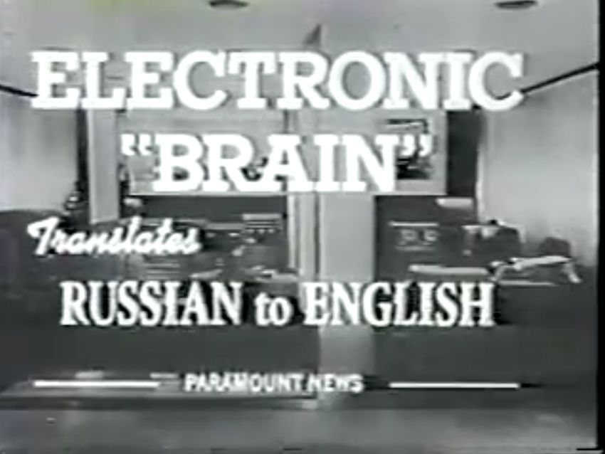
1950s: Early Machine Translation
Machine Translation research
began in the early 1950s.

• Russian → English
 (motivated by the Cold War!)

 1 minute video showing 1954 MT:
 https://youtu.be/K-HfpsHPmvw

• Systems were mostly rule-based, using a bilingual
 dictionary to map Russian words to their English
 counterparts

6

1990s-2010s: Statistical Machine Translation
• Core idea: Learn a probabilistic model from data
• Suppose we’re translating French → English.
• We want to find best English sentence y, given French sentence
 x

• Use Bayes Rule to break this down into two components to be
 learnt separately:

 Translation Model Language Model

 Models how words and phrases Models how to write
 should be translated (fidelity). good English (fluency).
 Learnt from parallel data. Learnt from monolingual
7 data.

1990s-2010s: Statistical Machine Translation
• Question: How to learn translation model ?
• First, need large amount of parallel data
 (e.g. pairs of human-translated French/English sentences)

 The Rosetta Stone
 Ancient Egyptian

 Demotic

 Ancient Greek

8

Learning alignment for SMT
• Question: How to learn translation model from
 the parallel corpus?

• Break it down further: Introduce latent a variable into the
 model:

 where a is the alignment, i.e. word-level correspondence
 between source sentence x and target sentence y

9

What is alignment?
Alignment is the correspondence between particular words in the translated sentence pair.

• Typological differences between languages lead to complicated alignments!
• Note: Some words have no counterpart

10 Examples from: “The Mathematics of Statistical Machine Translation: Parameter Estimation", Brown et al, 1993. http://www.aclweb.org/
 anthology/J93-2003

Alignment is complex
Alignment can be many-to-one

11 Examples from: “The Mathematics of Statistical Machine Translation: Parameter Estimation", Brown et al, 1993. http://www.aclweb.org/
 anthology/J93-2003

Alignment is complex
Alignment can be one-to-many

 Examples from: “The Mathematics of Statistical Machine Translation: Parameter Estimation", Brown et al, 1993. http://www.aclweb.org/
12 anthology/J93-2003

Alignment is complex
Some words are very fertile!
 he hit me with a pie

 il he il
 a hit a
 m’ me
 m’
 entarté with
 a entarté
 pie

This word has no single-
 word equivalent in
 English

13

Alignment is complex
Alignment can be many-to-many (phrase-level)

14 Examples from: “The Mathematics of Statistical Machine Translation: Parameter Estimation", Brown et al, 1993. http://www.aclweb.org/
 anthology/J93-2003

Learning alignment for SMT
• We learn as a combination of many factors,
 including:
 • Probability of particular words aligning (also depends on
 position in sent)
 • Probability of particular words having particular fertility
 (number of corresponding words)
 • etc.
• Alignments a are latent variables: They aren’t explicitly
 specified in the data!
 • Require the use of special learning aglos (like Expectation-
 Maximization) for learning the parameters of distributions
 with latent variables (CS 228)

15

Decoding for SMT

 Language Model
 Question:
 How to compute Translation
 this argmax? Model

• We could enumerate every possible y and calculate the
 probability? → Too expensive!
• Answer: Impose strong independence assumptions in model, use
 dynamic programming for globally optimal solutions (e.g. Viterbi
 algorithm).
• This process is called decoding

16

Viterbi: Decoding with Dynamic Programming
 • Impose strong independence assumptions in model:

 Source: “Speech and Language Processing", Chapter A, Jurafsky and Martin, 2019.

17

1990s-2010s: Statistical Machine Translation
• SMT was a huge research field
• The best systems were extremely complex
 • Hundreds of important details we haven’t mentioned
 here
 • Systems had many separately-designed subcomponents
 • Lots of feature engineering
 • Need to design features to capture particular language
 phenomena
 • Require compiling and maintaining extra resources
 • Like tables of equivalent phrases
 • Lots of human effort to maintain
 • Repeated effort for each language pair!

18

Section 2: Neural Machine Translation

19

What is Neural Machine Translation?
• Neural Machine Translation (NMT) is a way to do Machine
 Translation with a single neural network

• The neural network architecture is called sequence-to-
 sequence (aka seq2seq) and it involves two RNNs.

20

Neural Machine Translation (NMT)
 The sequence-to-sequence model
 Target sentence (output)
 Encoding of the source sentence.
 Provides initial hidden state
 he hit me with a pie 
 for Decoder RNN.

 argmax

 argmax

 argmax

 argmax

 argmax
 argmax

 argmax
Encoder RNN

 Decoder RNN
 il a m’ entarté he hit me with a pie

 Source sentence (input) Decoder RNN is a Language Model that
 generates target sentence, conditioned on
 encoding.
 Encoder RNN produces
 Note: This diagram shows test time behavior:
 an encoding of the decoder output is fed in as next step’s input
 source sentence.
 21

Sequence-to-sequence is versatile!
• Sequence-to-sequence is useful for more than just MT

• Many NLP tasks can be phrased as sequence-to-sequence:
 • Summarization (long text → short text)
 • Dialogue (previous utterances → next utterance)
 • Parsing (input text → output parse as sequence)
 • Code generation (natural language → Python code)

22

Neural Machine Translation (NMT)
• The sequence-to-sequence model is an example of a
 Conditional Language Model.
 • Language Model because the decoder is predicting the
 next word of the target sentence y
 • Conditional because its predictions are also conditioned on the
 source sentence x

• NMT directly calculates :

 Probability of next target word, given
 target words so far and source
 sentence x
• Question: How to train a NMT system?
• Answer: Get a big parallel corpus…
23

Training a Neural Machine Translation system
 = negative log = negative log = negative log
 prob of “he” prob of “with” prob of 
 1
 ∑
 = = 1 + 2 + 3 + 4 + 5 + 6 + 7
 =1

 ^1 ^2 ^3 ^4 ^5 ^6 ^7
Encoder RNN

 Decoder RNN
 il a m’ entarté he hit me with a pie

 Source sentence (from corpus) Target sentence (from corpus)

 Seq2seq is optimized as a single system.
 24 Backpropagation operates “end-to-end”.

Greedy decoding
• We saw how to generate (or “decode”) the target sentence
 by taking argmax on each step of the decoder

 he hit me with a pie 

 argmax

 argmax

 argmax

 argmax

 argmax
 argmax

 argmax

 he hit me with a
 pie
• This is greedy decoding (take most probable word on each
 step)
• Problems with this method?
25

Problems with greedy decoding
• Greedy decoding has no way to undo decisions!
 • Input: il a m’entarté (he hit me with a pie)
 • → he ____
 • → he hit ____
 • → he hit a ____ (whoops! no going back now…)

• How to fix this?

26

Exhaustive search decoding
• Ideally we want to find a (length T) translation y that
 maximizes

• We could try computing all possible sequences y
 • This means that on each step t of the decoder, we’re tracking Vt
 possible partial translations, where V is vocab size
 • This O(VT) complexity is far too expensive!

27

Beam search decoding
• Core idea: On each step of decoder, keep track of the k most
 probable partial translations (which we call hypotheses)
 • k is the beam size (in practice around 5 to 10)

• A hypothesis has a score which is its log
 probability:

 • Scores are all negative, and higher score is better
 • We search for high-scoring hypotheses, tracking top k on each step

• Beam search is not guaranteed to find optimal solution
• But much more efficient than exhaustive search!
28

Beam search decoding: example
 Beam size = k = 2. Blue numbers =

 Calculate prob
 29 dist of next word

Beam search decoding: example
 Beam size = k = 2. Blue numbers =

 -0.7 = log PLM(he|)
 he

 I
 -0.9 = log PLM(I|)

 Take top k words
 30 and compute scores

Beam search decoding: example
 Beam size = k = 2. Blue numbers =

 -1.7 = log PLM(hit| he) + -0.7
 -0.7 hit
 he
 struck
 -2.9= log PLM(struck| he) + -0.7

 -1.6= log PLM(was| I) + -0.9
 was
 I
 got
 -0.9
 -1.8 = log PLM(got| I) + -0.9
 For each of the k hypotheses, find
 31 top k next words and calculate scores

Beam search decoding: example
 Beam size = k = 2. Blue numbers =

 -1.7
 -0.7 hit
 he
 struck
 -2.9

 -1.6
 was
 I
 got
 -0.9
 -1.8
 Of these k2 hypotheses,
 32 just keep k with highest scores

Beam search decoding: example
 Beam size = k = 2. Blue numbers =

 -2.8 = log PLM(a| he hit) + -1.7
 -1.7 a
 -0.7 hit
 he me
 struck -2.5 = log PLM(me| he hit) + -1.7
 -2.9
 -2.9 = log PLM(hit| I was) + -1.6
 -1.6
 hit
 was
 I struck
 got
 -0.9 -3.8 = log PLM(struck| I was) + -1.6
 -1.8
 For each of the k hypotheses, find
 33 top k next words and calculate scores

Beam search decoding: example
 Beam size = k = 2. Blue numbers =

 -2.8
 -1.7 a
 -0.7 hit
 he me
 struck -2.5
 -2.9
 -2.9
 -1.6
 hit
 was
 I struck
 got
 -0.9 -3.8
 -1.8
 Of these k2 hypotheses,
 34 just keep k with highest scores

Beam search decoding: example
 Beam size = k = 2. Blue numbers =

 -4.0
 tart
 -2.8
 -1.7 pie
 a
 -0.7 -3.4
 hit
 he me -3.3
 struck -2.5 with
 -2.9
 -2.9 on
 -1.6
 hit -3.5
 was
 I struck
 got
 -0.9 -3.8
 -1.8
 For each of the k hypotheses, find
 35 top k next words and calculate scores

Beam search decoding: example
 Beam size = k = 2. Blue numbers =

 -4.0
 tart
 -2.8
 -1.7 pie
 a
 -0.7 -3.4
 hit
 he me -3.3
 struck -2.5 with
 -2.9
 -2.9 on
 -1.6
 hit -3.5
 was
 I struck
 got
 -0.9 -3.8
 -1.8
 Of these k2 hypotheses,
 36 just keep k with highest scores

Beam search decoding: example
 Beam size = k = 2. Blue numbers =

 -4.0 -4.8
 tart in
 -2.8
 -1.7 pie with
 a
 -0.7 -3.4 -4.5
 hit
 he me -3.3 -3.7
 struck -2.5 with a
 -2.9
 -2.9 on one
 -1.6
 hit -3.5 -4.3
 was
 I struck
 got
 -0.9 -3.8
 -1.8
 For each of the k hypotheses, find
 37 top k next words and calculate scores

Beam search decoding: example
 Beam size = k = 2. Blue numbers =

 -4.0 -4.8
 tart in
 -2.8
 -1.7 pie with
 a
 -0.7 -3.4 -4.5
 hit
 he me -3.3 -3.7
 struck -2.5 with a
 -2.9
 -2.9 on one
 -1.6
 hit -3.5 -4.3
 was
 I struck
 got
 -0.9 -3.8
 -1.8
 Of these k2 hypotheses,
 38 just keep k with highest scores

Beam search decoding: example
 Beam size = k = 2. Blue numbers =

 -4.0 -4.8
 tart in
 -2.8 -4.3
 -1.7 pie with
 a pie
 -0.7 -3.4 -4.5
 hit
 he me -3.3 -3.7 tart
 struck -2.5 with a -4.6
 -2.9
 -2.9 on one -5.0
 -1.6
 hit -3.5 -4.3 pie
 was
 I struck tart
 got
 -0.9 -3.8 -5.3
 -1.8
 For each of the k hypotheses, find
 39 top k next words and calculate scores

Beam search decoding: example
 Beam size = k = 2. Blue numbers =

 -4.0 -4.8
 tart in
 -2.8 -4.3
 -1.7 pie with
 a pie
 -0.7 -3.4 -4.5
 hit
 he me -3.3 -3.7 tart
 struck -2.5 with a -4.6
 -2.9
 -2.9 on one -5.0
 -1.6
 hit -3.5 -4.3 pie
 was
 I struck tart
 got
 -0.9 -3.8 -5.3
 -1.8

 40 This is the top-scoring hypothesis!

Beam search decoding: example
 Beam size = k = 2. Blue numbers =

 -4.0 -4.8
 tart in
 -2.8 -4.3
 -1.7 pie with
 a pie
 -0.7 -3.4 -4.5
 hit
 he me -3.3 -3.7 tart
 struck -2.5 with a -4.6
 -2.9
 -2.9 on one -5.0
 -1.6
 hit -3.5 -4.3 pie
 was
 I struck tart
 got
 -0.9 -3.8 -5.3
 -1.8

 41 Backtrack to obtain the full hypothesis

Beam search decoding: stopping criterion
• In greedy decoding, usually we decode until the model
 produces a token
 • For example: he hit me with a pie 

• In beam search decoding, different hypotheses may
 produce tokens on different timesteps
 • When a hypothesis produces , that hypothesis is complete.
 • Place it aside and continue exploring other hypotheses via beam
 search.

• Usually we continue beam search until:
 • We reach timestep T (where T is some pre-defined cutoff), or
 • We have at least n completed hypotheses (where n is pre-defined
 cutoff)

42

Beam search decoding: finishing up
• We have our list of completed hypotheses.
• How to select top one with highest score?

• Each hypothesis on our list has a score

• Problem with this: longer hypotheses have lower scores

• Fix: Normalize by length. Use this to select top one
 instead:

43

Advantages of NMT
Compared to SMT, NMT has many advantages:

• Better performance
 • More fluent
 • Better use of context
 • Better use of phrase similarities

• A single neural network to be optimized end-to-end
 • No subcomponents to be individually optimized

• Requires much less human engineering effort
 • No feature engineering
 • Same method for all language pairs

44

Disadvantages of NMT?
Compared to SMT:

• NMT is less interpretable
 • Hard to debug

• NMT is difficult to control
 • For example, can’t easily specify rules or guidelines for
 translation
 • Safety concerns!

45

How do we evaluate Machine Translation?
BLEU (Bilingual Evaluation Understudy) You’ll see BLEU in
 detail in Assignment
 4!
• BLEU compares the machine-written translation to one or
 several human-written translation(s), and computes a
 similarity score based on:
 • n-gram precision (usually for 1, 2, 3 and 4-grams)
 • Plus a penalty for too-short system translations

• BLEU is useful but imperfect
 • There are many valid ways to translate a sentence
 • So a good translation can get a poor BLEU score because
 it has low n-gram overlap with the human translation ☹

46 Source: ”BLEU: a Method for Automatic Evaluation of Machine Translation", Papineni et al, 2002. http://aclweb.org/anthology/P02-1040

MT progress over time
 [Edinburgh En-De WMT newstest2013 Cased BLEU; NMT 2015 from U. Montréal]

 27 Phrase-based SMT Syntax-based SMT
 Neural MT

20.3

13.5

 6.8

 0
 2013 2014 2015 2016

 47 Source: http://www.meta-net.eu/events/meta-forum-2016/slides/09_sennrich.pdf

MT progress over time

48

NMT: the biggest success story of NLP Deep Learning

Neural Machine Translation went from a fringe research
activity in 2014 to the leading standard method in 2016

• 2014: First seq2seq paper published

• 2016: Google Translate switches from SMT to NMT

• This is amazing!
 • SMT systems, built by hundreds of engineers over many
 years, outperformed by NMT systems trained by a
 handful of engineers in a few months

49

So is Machine Translation solved?
• Nope!
• Many difficulties remain:
 • Out-of-vocabulary words
 • Domain mismatch between train and test data
 • Maintaining context over longer text
 • Low-resource language pairs

 Further reading: “Has AI surpassed humans at translation? Not even close!”
50 https://www.skynettoday.com/editorials/state_of_nmt

So is Machine Translation solved?
 • Nope!
 • Using common sense is still hard
 • Idioms are difficult to translate

51

So is Machine Translation solved?
• Nope!
• NMT picks up biases in training data

 Didn’t specify gender

52 Source: https://hackernoon.com/bias-sexist-or-this-is-the-way-it-should-be-
 ce1f7c8c683c

So is Machine Translation solved?
• Nope!
• Uninterpretable systems do strange things

 Picture source: https://www.vice.com/en_uk/article/j5npeg/why-is-google-translate-spitting-out-sinister-
53 religious-prophecies
 Explanation: https://www.skynettoday.com/briefs/google-nmt-prophecies

NMT research continues
NMT is the flagship task for NLP Deep Learning

• NMT research has pioneered many of the recent innovations
 of NLP Deep Learning

• In 2019: NMT research continues to thrive
 • Researchers have found many, many improvements to the
 “vanilla” seq2seq NMT system we’ve presented today
 • But one improvement is so integral that it is the new
 vanilla…

 ATTENTION
54

Section 3: Attention

55

Sequence-to-sequence: the bottleneck problem
 Encoding of the
 source sentence.
 Target sentence (output)

 he hit me with a pie 
Encoder RNN

 Decoder RNN
 il a m’ entarté he hit me with a pie

 Source sentence (input)

 Problems with this architecture?

 56

Sequence-to-sequence: the bottleneck problem
 Encoding of the
 source sentence.
 This needs to capture all Target sentence (output)
 information about the
 source sentence.
 Information bottleneck! he hit me with a pie
 
Encoder RNN

 Decoder RNN
 il a m’ he hit me with a
 entarté pie

 Source sentence (input)

 57

Attention
• Attention provides a solution to the bottleneck problem.

• Core idea: on each step of the decoder, use direct
 connection to the encoder to focus on a particular part of
 the source sequence

• First we will show via diagram (no equations), then we will
 show with equations

58

Sequence-to-sequence with attention

 dot product
Encoder Attention
 scores

 Decoder RNN
 RNN

 il a m’ entarté 

 59 Source sentence (input)

Sequence-to-sequence with attention

 dot product
Encoder Attention
 scores

 Decoder RNN
 RNN

 il a m’ entarté 

 60 Source sentence (input)

Sequence-to-sequence with attention

 dot product
Encoder Attention
 scores

 Decoder RNN
 RNN

 il a m’ entarté 

 61 Source sentence (input)

Sequence-to-sequence with attention

 dot product
Encoder Attention
 scores

 Decoder RNN
 RNN

 il a m’ entarté 

 62 Source sentence (input)

Sequence-to-sequence with attention

 On this decoder timestep,
 we’re mostly focusing on the
 scores distribution
Encoder Attention Attention

 first encoder hidden state
 (”he”)

 Take softmax to turn the
 scores into a probability
 distribution

 Decoder RNN
 RNN

 il a m’ entarté 

 63 Source sentence (input)

Sequence-to-sequence with attention
 Attention Use the attention distribution to take
 output a weighted sum of the encoder
 hidden states.
 scores distribution
Encoder Attention Attention

 The attention output mostly contains
 information from the hidden states
 that received high attention.

 Decoder RNN
 RNN

 il a m’ entarté 

 64 Source sentence (input)

Sequence-to-sequence with attention
 Attention he
 output
 Concatenate attention output
 ^1
 scores distribution

 with decoder hidden state,
Encoder Attention Attention

 then use to compute as
 before

 Decoder RNN
 RNN

 il a m’ entarté 

 65 Source sentence (input)

Sequence-to-sequence with attention
 Attention hit
 output
 ^2
 scores distribution
Encoder Attention Attention

 Decoder RNN
 RNN

 Sometimes we take the
 attention output from
 the previous step, and
 also feed it into the
 he decoder (along with the
 il a m’ entarté
 usual decoder input).
 We do this in
 66 Source sentence (input) Assignment 4.

Sequence-to-sequence with attention
 Attention me
 output
 ^3
 scores distribution
Encoder Attention Attention

 Decoder RNN
 RNN

 il a m’ entarté he hit

 67 Source sentence (input)

Sequence-to-sequence with attention
 Attention with
 output
 ^4
 scores distribution
Encoder Attention Attention

 Decoder RNN
 RNN

 il a m’ entarté he hit me

 68 Source sentence (input)

Sequence-to-sequence with attention
 Attention a
 output
 ^5
 scores distribution
Encoder Attention Attention

 Decoder RNN
 RNN

 il a m’ entarté he hit me with

 69 Source sentence (input)

Sequence-to-sequence with attention
 Attention pie
 output
 ^6
 scores distribution
Encoder Attention Attention

 Decoder RNN
 RNN

 il a m’ entarté he hit me with a

 70 Source sentence (input)

Attention: in equations
• We have encoder hidden states
• On timestep t, we have decoder hidden state
• We get the attention scores for this step:

• We take softmax to get the attention distribution for this step
 (this is a probability distribution and sums to 1)

• We use to take a weighted sum of the encoder hidden states to
 get the attention output

• Finally we concatenate the attention output with the decoder
 hidden state and proceed as in the non-attention seq2seq model

71

Attention is great
• Attention significantly improves NMT performance
 • It’s very useful to allow decoder to focus on certain parts of the
 source
• Attention solves the bottleneck problem
 • Attention allows decoder to look directly at source; bypass bottleneck
• Attention helps with vanishing gradient problem
 • Provides shortcut to faraway states
• Attention provides some interpretability
 he hit me wit a pie
 • By inspecting attention distribution, we can see h
 what the decoder was focusing on il

 • We get (soft) alignment for free! a

 m’
 • This is cool because we never explicitly trained
 entarté
 an alignment system
 • The network just learned alignment by itself

72

Attention is a general Deep Learning technique
• We’ve seen that attention is a great way to improve the
 sequence-to-sequence model for Machine Translation.
• However: You can use attention in many architectures
 (not just seq2seq) and many tasks (not just MT)

• More general definition of attention:
 • Given a set of vector values, and a vector query, attention
 is a technique to compute a weighted sum of the values,
 dependent on the query.

• We sometimes say that the query attends to the values.
• For example, in the seq2seq + attention model, each decoder
 hidden state (query) attends to all the encoder hidden states
 (values).
73

Attention is a general Deep Learning technique
More general definition of attention:
Given a set of vector values, and a vector query, attention
is a technique to compute a weighted sum of the values,
dependent on the query.

Intuition:
 • The weighted sum is a selective summary of the
 information contained in the values, where the query
 determines which values to focus on.
 • Attention is a way to obtain a fixed-size representation
 of an arbitrary set of representations (the values),
 dependent on some other representation (the query).

74

There are several attention variants
• We have some values and a query

• Attention always involves:
 There are
 1. Computing the attention scores multiple ways
 2. Taking softmax to get attention distribution ⍺: to do this

 3. Using attention distribution to take weighted sum of
 values:

 thus obtaining the attention output a (sometimes called
 the context vector)
75

You’ll think about the relative advantages/
Attention variants disadvantages of these in Assignment 4!

There are several ways you can compute from
and :

• Basic dot-product attention:
 • Note: this assumes
 • This is the version we saw earlier

• Multiplicative attention:
 • Where is a weight matrix

• Additive attention:
 • Where are weight matrices and
 is a weight vector.
 • d3 (the attention dimensionality) is a hyperparameter
 More information:
 “Deep Learning for NLP Best Practices”, Ruder, 2017. http://ruder.io/deep-learning-nlp-best-practices/
76 index.html#attention
 “Massive Exploration of Neural Machine Translation Architectures”, Britz et al, 2017, https://arxiv.org/pdf/
 1703.03906.pdf

Summary of today’s lecture
• We learned some history of Machine Translation (MT)

• Since 2014, Neural MT rapidly
 replaced intricate Statistical MT

• Sequence-to-sequence is the
 architecture for NMT (uses 2 RNNs)

• Attention is a way to focus on
 particular parts of the input
 • Improves sequence-to-sequence a lot!
77