New Ground Motion to Intensity Conversion Equations for China
←
→
Page content transcription
If your browser does not render page correctly, please read the page content below

Hindawi
Shock and Vibration
Volume 2021, Article ID 5530862, 21 pages
https://doi.org/10.1155/2021/5530862

Research Article
New Ground Motion to Intensity Conversion Equations for China

 Xiufeng Tian ,1,2 Zengping Wen,1 Weidong Zhang,2 and Jie Yuan2
 1
 Institute of Geophysics, China Earthquake Administration, Beijing 10081, China
 2
 Gansu Earthquake Agency, Lanzhou 73000, Gansu, China

 Correspondence should be addressed to Xiufeng Tian; txf913@163.com

 Received 18 February 2021; Revised 28 June 2021; Accepted 21 July 2021; Published 29 July 2021

 Academic Editor: Sara Amoroso

 Copyright © 2021 Xiufeng Tian et al. This is an open access article distributed under the Creative Commons Attribution License,
 which permits unrestricted use, distribution, and reproduction in any medium, provided the original work is properly cited.

 In this study, we use the strong motion records and seismic intensity data from 11 moderate-to-strong earthquakes in the
 mainland of China since 2008 to develop new conversion equations between seismic intensity and peak ground motion pa-
 rameters. Based on the analysis of the distribution of the dataset, the reversible conversion relationships between modified
 Mercalli intensity (MMI) and peak ground acceleration (PGA), peak ground velocity (PGV), and pseudo-spectral acceleration
 (PSA) at natural vibration periods of 0.3 s, 1.0 s, 2.0 s, and 3.0 s are obtained by using the orthogonal regression. The influence of
 moment magnitude, hypocentral distance, and hypocentral depth on the residuals of conversion equations is also explored. To
 account for and eliminate the trends in the residuals, we introduce a magnitude-distance-depth correction term and obtain the
 improved relationships. Furthermore, we compare the results of this study with previously published works and analyze the
 regional dependence of conversion equations. To quantify the regional variations, a regional correction factor for China, suitable
 for adjustment of global relationships, has also been estimated.

1. Introduction In some countries or regions with abundant seismic
 records (e.g., the United States, Japan, Italy, Turkey, New
As a qualitative index to describe the ground vibration and Zealand, and Taiwan), researchers have explored the cor-
degree of damage caused by an earthquake, the seismic intensity relation between seismic intensity and ground motion pa-
provides a simple macroscopic scale to characterize the mag- rameters and established the corresponding ground motion
nitude of an earthquake’s impact on human communities, so it to intensity conversion equations (GMICEs) [3–12]. At
is widely used in earthquake disaster assessment, loss estima- present, there are numerous seismic intensity scales, such as
tion, structural response analyses, historical earthquake disaster modified Mercalli intensity (MMI), Mercalli–Cancani–Sie-
recurrence, and other fields all over the world [1]. Traditionally, berg (MCS) intensity, JMA intensity in Japan, and so on in
seismic intensity is typically obtained by experts who investigate which MMI is the most widely used. With respect to these
the building damage and human response to an earthquake in seismic intensity scales, most researchers calibrate their
an area where that earthquake strikes. Ground motion pa- conversion equations using PGA, PGV, and PSA as physical
rameters, such as PGA, PGV, and PSA, which are used as indicators. In early works, PGA was employed as the ground
quantitative indexes to describe the degree of ground vibration, motion parameter that would provide accurate seismic in-
are usually obtained from the records of seismic observation tensity estimates because it was assumed that the product of
instruments deployed in earthquake areas. How to transform acceleration and mass would accurately characterize the
the ground motion parameters into seismic intensity and es- inertial forces acting on the structure [13–15]. However,
tablish the conversion equation between them is of great sig- because PGV is directly related to the kinetic energy, some
nificance for the rapid assessment of earthquake disaster and studies have found that the correlation between PGV and
loss (such as the generation of ShakeMap [2]), the comparative seismic intensity is stronger than it is for PGA [16, 17]. Wald
analysis of different types of intensity scales, and other engi- et al. proposed that low seismic intensities were strongly
neering applications. correlated to both PGA and PGV, while high seismic
2 Shock and Vibration

intensities were only strongly correlated with PGV [3]. Bilal data. (2) With the rapid development of national economy, the
and Askan concluded that the seismic intensity was more structure of buildings, seismic resistance, and the types of
closely related to PGV for ductile structures and PGA for earthquake damage have changed significantly, and the dis-
brittle structures [8]. For the response spectrum parameters, tribution of the peak ground motion corresponding to the
which are directly related to the seismic response and seismic intensity may also change accordingly. Thus, in this
structural damage, many researchers found that they were study, we intend to use the recent seismic dataset of China and
also closely related to seismic intensity. As Spence et al. develop the new conversion equations between seismic intensity
demonstrated, the correlation between seismic intensity and and PGA, PGV, and PSA.
PSA (5% damping ratio) over a period of 0.1 s to 0.3 s was
stronger than it is for PGA [18]. Boatwright et al. determined 2. Data Source and Analysis
that seismic intensity correlated best with the velocity re-
sponse spectra (5% damping ratio) at a period of 1.5 s [19]. In 2.1. Data Source. In this study, the seismic data consist of the
addition, Caprio et al. derived new global relationships, strong motion records from 11 moderate-to-strong earth-
assembling a database from active crustal regions in Cal- quakes (5.9 ≤ Mw ≤ 7.9) that occurred in the mainland of
ifornia, Italy, Greece, and global data from the Central and China from 2008 to 2019. We downloaded the data from the
Eastern United States catalog. The authors obtained the PGA China Strong Motion Network Center (see Data Avail-
and PGV to intensity conversion equations and provided ability), which used a new digital strong motion network
regional correction factors to the global relationships for after 2008, and obtained a large volume of strong motion
Italy, Greece, and California, as well as a regional similarity data from destructive earthquakes. The locations of the 11
study for other regions of the world [10]. Moratalla et al. earthquakes as well as the spatial distribution of the strong
considered a large amount of data derived from New motion stations that recorded these events are displayed in
Zealand earthquakes and developed the updated GMICEs Figure 1, the detailed information of these earthquake events
between MMI and PGA/PGV [11]. The work also proposed a is given in Table 1, and the magnitude versus hypocentral
regional correction factor for New Zealand, suitable for the distance distribution of the dataset is shown in Figure 2. We
global relationships of Caprio et al. [10]. employ the method of Yu et al. [23] to perform baseline
 The research on the correlation between seismic intensity correction and filtering and obtain PGA, PGV, and PSA (5%
and ground motion parameters in China began in the 1960s. damping ratio) at natural vibration periods of 0.3 s, 1.0 s,
The intensity scale used was MMI, and the PGA value corre- 2.0 s, and 3.0 s of the two horizontal components for each
sponding to the intensity of VII-IX was given in the seismic record. The maximum value of the two horizontal com-
building design code at that time. Due to the lack of local strong ponents is used in the subsequent regression analysis.
motion records in China, Liu et al. used a small amount of The macroseismic intensity data (in terms of MMI scale)
seismic data from the United States and some foreign research were compiled from the isoseismal maps and damage re-
results [20], took PGA and PGV as the measures of seismic ports of the past earthquakes (see Data Availability). The
intensity, and gave the conversion equations between MMI and isoseismal maps were obtained by detailed post-earthquake
PGA/PGV [21], which were applied in Chinese seismic intensity survey and site evaluations after the earthquakes at the
scale in 1980. Du et al. derived a new empirical relationship meizoseismal areas by reconnaissance teams. All the maps
between MMI and PGA/PGV for Western China, using the and bulletins used in this paper were prepared by the China
ground motion records of earthquakes that occurred before Earthquake Administration, involving the MMI range from
2014 [22]. The work used a weighted least-squares regression V to X. For the past earthquakes with an observed isoseismal
method, resulting in an irreversible conversion from PGA/PGV map or a detailed earthquake damage report from which
to MMI, and the relationship between MMI and PSA was not MMI values were easy to obtain, the peak ground motion
considered in the literature. It is worth noting that the con- corresponding to MMI can be paired straightforwardly. We
version equations from PGA/PGV to MMI are not scrutinized assigned one MMI value for each recorded accelerogram
and revised by using recent local seismic data; in addition, as of considering the location of accelerograph stations on the
now, the robust correlation relationships between MMI and isoseismal maps or considering the observed intensity value
PSA, which are also very useful because the spectral quantities near the stations (≤2 km), and a total of 242 peak ground
are strong indicators of the structural response which directly motion-intensity pairs were obtained.
influence the observed intensity values, have not been studied in
detail for Chinese earthquake dataset. So, there is an urgent need
to re-examine the GMICEs in China thoroughly and develop 2.2. Data Analysis. Using the seismic dataset described in
the updated relationships using the latest local seismic data and the previous section, we have calculated the max, min, and
including PSA in addition to PGA and PGV. Furthermore, two mean values, as well as the standard deviations of PGA,
realistic factors also inspire us to develop the new GMICEs. (1) PGV, and PSA (hereafter denoted as PGM, i.e., peak ground
Since 2008, the operation of China Digital Strong Motion motion) in logarithmic scale for different intensity units
Network has greatly increased the quantity and quality of the ranging from V to X (Table 2). It can be seen from Table 2
strong motion observation stations, and in recent years, the that the discreteness of seismic parameters in each intensity
mainland of China has experienced a number of moderate-to- unit is very large, but the mean value has a good positive
strong destructive earthquakes, resulting in large volumes of correlation with the intensity value. We also draw the fre-
strong motion records and post-earthquake seismic intensity quency distribution of the datapoints in each intensity unit

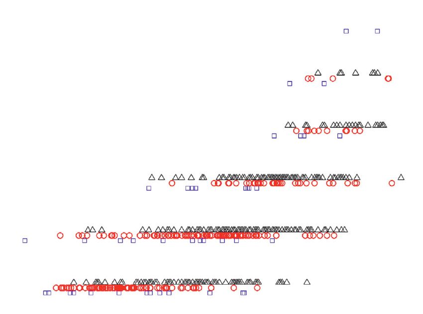
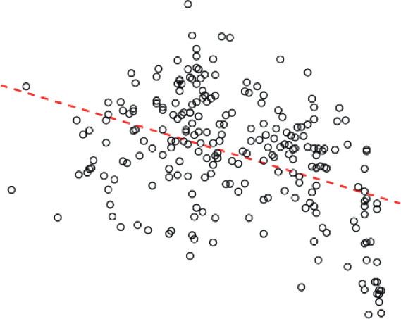
Shock and Vibration 3

 90° E 100° E 110° E

 km
 0 65130 260 390 520 N
 40° N

 40° N
 30° N

 30° N
 Strong motion station
 Epicenter of earthquake

 90° E 100° E
 Figure 1: Locations of earthquake events and strong motion stations used in this study.

for logPGM (Figures 3 and 4, for PGA and PGV; Figures that of America and larger than that of Turkey, and the PGV
5–8, for PSA). From these figures, we can see that the sample of Chinese data is smaller than that of America and Turkey.
data in intensity units of V to VII have approximate nor- This regional difference of the data distribution indicates
mality, which is less obvious in the intensity units of VIII to that the GMICEs for a certain area must be obtained using
IX due to its smaller amount of data. It also should be noted the local seismic dataset, and the introduction of nonlocal
that the mode and mean values of PGA (Figure 3) in each seismic data may lead to inaccurate results. Therefore, only
intensity unit in our dataset are evidently higher than the the seismic dataset of China (Table 1) is used in this study to
corresponding values of Liu et al. [21]. This significant obtain the most suitable GMICEs for local use.
finding further illustrates the necessity to re-examine the
GMICEs used in China and make necessary improvements.
 In addition, the dataset in this study is also compared
 3. Regression Analysis
with the datasets of America and Turkey [2–5, 8] (Figure 9, 3.1. Outlier Test of Data. To ensure the accuracy of the re-
taking PGA and PGV as examples). It can be seen from gression results, it is necessary to screen and delete outliers
Figure 9 that the distribution of Chinese data is inconsistent from our dataset prior to the statistical analyses. Because the
with that of the other two regions. As a whole, the PGA of conversion equations between MMI and PGM are usually
Chinese data in each of the intensity units is smaller than characterized by a linear function with respect to logPGM, it
4 Shock and Vibration

 Table 1: List of earthquake events.
 Number of MMI- Hypocentral
Serial Earthquake Event Latitude Longitude Magnitude Hypocentral
 PGA, PGV, and PSA distance range
number name date (°N) (°E) (Mw) depth (km)
 pairs (km)
 2008-
1 Wenchuan 31.01 103.42 7.9 14 134 27.0–640.5
 05-12
 2012-
2 Xinyuan 43.42 84.74 6.6 7 11 68.6–193.2
 06-30
 2013-
3 Lushan 30.30 103.00 7.0 13 22 26.1–146.8
 04-20
 Minxian- 2013-
4 34.54 104.21 6.6 15 13 26.0–112.1
 Zhangxian 07-22
 2014-
5 Ludian 27.11 103.33 6.5 10 19 11.2–87.4
 08-03
 2014-
6 Jinggu 23.40 100.55 6.6 10 9 18.4–81.8
 10-07
 2014-
7 Kangding 30.29 101.68 6.3 20 9 38.4–95.2
 11-22
 2016-
8 Menyuan 37.68 101.62 6.4 10 6 32.1–91.0
 01-21
 2016-
9 Hutubi 43.83 86.35 6.3 6 8 13.3–99.4
 12-08
 2017-
10 Jiuzhaigou 33.20 103.82 7.0 20 8 32.1–110.6
 08-08
 2019-
11 Changning 28.34 104.90 5.9 16 3 23.4–52.9
 06-17

 8.0

 7.5

 7.0
 Mw

 6.5

 6.0

 5.5
 1 10 100 1000
 Hypocentral distance (km)

 Figure 2: Distribution of ground motion dataset regarding magnitude and hypocentral distance.

is necessary to search for outliers in the dataset of loga- According to the test results, we find only one straggler
rithmic scale for each intensity unit. of logPGA value (0.38), which came from the 51BTD station
 Because the sample data of logPGM in most of the located at the intensity V region in the 2014 Mw6.5 Ludian
intensity units approximately obey the normal distribu- earthquake. This station, consisting of a MR2002/SLJ-100
tion, according to the recommendations in Chinese Na- seismometer, is located in Butuo County, Liangshan Pre-
tional Standard GB/T 4883-2008 (Statistical fecture, Sichuan Province. Its Vs30 is 368.12 m/s, and the
Interpretation of Data: Detection and Treatment of observation site is the soil layer. Butuo County is built on a
Outliers in the Normal Sample) [24], we conduct the valley with special topography, which may lead to an ab-
skewness-kurtosis test on sample data in intensity units normal PGA value that should be deleted from our dataset. It
ranging from V to VII because of the high number of is also worth noting that the sample data of MMI X are not
samples in these intensity units. Conversely, there are used in the subsequent analysis, which is because we use the
fewer sample data in the intensity units of VIII and IX, and mean value of the sample data in each intensity unit to
the Dixon test is used to identify the outliers. In addition, develop the regression but there is only one sample data in
the outlier test is not performed for the intensity unit of X MMI X. To avoid the fitting deviation caused by the single
because there is only one sample data in this intensity unit. data and ensure the overall stability of the regression results,

Shock and Vibration 5

 Table 2: Summary of statistical values for each of the intensity units.
 MMI logPGA logPGV logPSA (0.3 s) logPSA (1.0 s) logPSA (2.0 s) logPSA (3.0 s) Number of data points
 Max 2.14 1.31 2.66 2.08 2.16 1.93
 Min 0.38 −0.33 0.64 0.45 0.00 −0.03
V 90
 Mean 1.40 0.54 1.74 1.46 1.32 1.11
 St.dev 0.28 0.37 0.32 0.39 0.48 0.46
 Max 2.63 1.44 2.89 2.43 2.41 2.03
 Min 0.88 −0.23 1.31 0.79 0.47 0.31
VI 96
 Mean 1.96 0.84 2.27 1.82 1.51 1.24
 St.dev 0.37 0.32 0.35 0.38 0.40 0.38
 Max 3.00 1.62 3.18 2.53 2.15 1.95
 Min 1.60 0.53 2.01 1.36 0.97 0.80
VII 40
 Mean 2.35 1.11 2.66 2.00 1.62 1.40
 St.dev 0.28 0.27 0.31 0.29 0.29 0.28
 Max 2.80 1.80 3.37 2.97 2.34 2.01
 Min 2.39 1.14 2.58 2.01 1.42 1.42
VIII 10
 Mean 2.61 1.46 2.97 2.53 2.03 1.81
 St.dev 0.14 0.20 0.23 0.32 0.32 0.26
 Max 2.98 1.96 3.37 3.05 2.64 2.49
 Min 2.47 1.34 2.86 2.24 1.87 1.70
IX 5
 Mean 2.77 1.74 3.11 2.73 2.28 2.05
 St.dev 0.26 0.28 0.23 0.34 0.29 0.32
 Max
 Min
X 2.91 1.95 2.97 2.72 2.49 2.42 1
 Mean
 St.dev

we delete the data of MMI X from our dataset. As such, our Given the reversibility of the equation, the equation for
conversion equations are only applicable within the intensity calculating PGM from MMI is
range of V ≤ MMI ≤ IX.
 MMI − c2
 logPGM � . (2)
 c1
3.2. Regression Results. In this present study, the orthogonal Table 3 provides a summary of the coefficients in
regression, which is also known as total least square re- equations (1) and (2), as well as the corresponding standard
gression or Deming regression [25], has been used to fit our deviations of the residuals obtained by applying these
MMI-logPGM data pairs and develop the GMICEs for equations to the complete dataset, for both logPGM and
China. The orthogonal regression calculates the residuals as MMI. Regression lines for PGA and PGV are shown in
the minimum perpendicular distance from a point to the Figure 10 (regression lines for PSA are shown in Figure 11).
regression line. It considers the error on both the dependent In Figure 10(a), we take the MMI-PGA relationship
and independent variables and has an important advantage derived by Liu et al. [21] as a reference. It is clearly observed
for making the equations reversible. This is very useful for that there are significant differences between the two rela-
GMICEs because we can use the reverse equations to analyze tionships. Under the same value of PGA, the MMI calculated
the historical earthquakes which have only seismic intensity by the equation of Liu et al. [21] is greater than that obtained
information but no ground motion measure data. In ad- by the formula developed in this study. The possible reason is
dition, according to the statistical results described in the because nowadays the buildings in China are more earth-
previous section that the low intensity units have a large quake resistant than those in 1980. Similar trends can be
number of samples while the high intensity units have a found in the comparison of MMI-PGV relationships shown
small number of samples, we use the mean value of the in Figure 10(b), which is less obvious than that in
sample data in each intensity unit to develop the regression Figure 10(a).
to assure the equal weight for all intensity units.
 The GMICEs to estimate MMI from PGM are provided
in the following equation: 4. Residual Analysis for Magnitude, Distance,
 and Depth Dependence
 MMI � c1 · logPGM + c2 , (1)
 We perform a residual analysis of the dataset to identify
in which PGM corresponds to PGA, PGV, PSA (0.3 s), PSA possible trends related to earthquake magnitude, hypo-
(1.0 s), PSA (2.0 s), and PSA (0.3 s) and c1 and c2 are the central distance, and hypocentral depth. The objective is to
fitting coefficients, where c1 is the slope obtained from the quantify the dependence on these factors and calculate
linear regression and c2 is the intercept. residual corrections. Based on the regression relationships
6 Shock and Vibration

 25 14

 12
 20
 10
 Frequency

 Frequency
 15 8

 10 6

 4
 5
 2

 0 0
 0.6 0.9 1.2 1.5 1.8 2.1 0.9 1.2 1.5 1.8 2.1 2.4 2.7
 logPGA (MMI = V) logPGA (MMI = VI)
 20
 4

 15 3

 Frequency
 Frequency

 10 2

 5 1

 0 0
 1.6 1.8 2.0 2.2 2.4 2.6 2.8 3.0 2.3 2.4 2.5 2.6 2.7 2.8 2.9
 logPGA (MMI = VII) logPGA (MMI = VIII)

 2
 Frequency

 1

 0
 2.3 2.4 2.5 2.6 2.7 2.8 2.9 3.0 3.1
 logPGA (MMI = IX)
 Figure 3: Histograms of the distribution of logPGA.

in equation (1), we calculate the residuals of MMI values magnitude, which are obtained from linear least-squares fit.
(i.e., the difference between the observed MMI and the We then add this correction term to equation (1) and yield
predicted MMI) and plot the trends of residuals with an intermediate relationship:
moment magnitude, hypocentral distance, and hypocentral
 MMI � c1 · logPGM + c2 + c3 · M + ct1 . (4)
depth (Figures 12–14, for PGA and PGV; Figures 15–17, for
PSA). Secondly, using the intermediate relationship (equation
 To eliminate the dependence of residuals on magnitude, (4)), we calculate the new residuals of MMI values and
distance, and depth, it is necessary to introduce new vari- introduce the distance correction term:
ables into the prediction model (equation (1)). Here an
approach similar to Worden et al. [6] is adopted. Firstly, we cR � c4 · log R + ct2 , (5)
introduce the magnitude correction term:
 where R is the hypocentral distance and c4 and ct2 are the
 cM � c3 · M + ct1 , (3) parameters of the line defining the trend in residuals with
 distance. Similarly, the distance correction term is added
where M is the moment magnitude and c3 and ct1 are the to equation (4) to get an updated intermediate
parameters of the line defining the trend in residuals with relationship:
Shock and Vibration 7

 12 14

 10 12

 10
 8

 Frequency
 Frequency

 8
 6
 6
 4
 4
 2 2

 0 0
 -0.3 0.0 0.3 0.6 0.9 1.2 -0.3 0.0 0.3 0.6 0.9 1.2 1.5
 logPGV (MMI = V) logPGV (MMI = VI)

 10 5

 8 4
 Frequency

 Frequency
 6 3

 4 2

 2 1

 0 0
 0.5 0.8 1.1 1.4 1.7 1.1 1.2 1.3 1.4 1.5 1.6 1.7 1.8
 logPGV (MMI = VII) logPGV (MMI = VIII)

 1
 Frequency

 0
 1.3 1.4 1.5 1.6 1.7 1.8 1.9 2.0
 logPGV (MMI = IX)
 Figure 4: Histograms of the distribution of logPGV.

 MMI � c1 · logPGM + c2 + c3 · M + ct1 + c4 · log R + ct2 . Table 4 lists the fitted coefficients and the new standard
 deviations of residuals after applying the correction terms.
 (6) When we examine the residuals obtained using equation (8)
 Lastly, using this new relationship (equation (6)), we to predict MMI (instead of equation (1)), we note that the
calculate the depth correction term: trends have been removed. Moreover, as can be seen from a
 comparison of the sigma values in Table 4 with those in
 cD � c5 · D + ct3 , (7) Table 3, the inclusion of magnitude-distance-depth cor-
 rection terms reduces the standard deviations of the re-
where D is the hypocentral depth and c5 and ct3 are the
 siduals for all ground motion types.
parameters of the line defining the trend in residuals with
depth. Then, we can obtain the improved prediction
relationship: 5. Comparison of the Proposed GMICEs with
 Previous Studies
 MMI � c1 · logPGM + c2 + c3 · M + c4 · log R + c5 · D + c6 ,
 (8) The GMICEs developed in this study (equation (1)) are
 compared with similar relationships developed for different
where c6 � ct1 + ct2 + ct3. regions worldwide [2, 4, 5, 7, 8, 10–12, 17, 20–22, 26–28] to
8 Shock and Vibration

 25 25

 Frequency 20 20

 Frequency
 15 15

 10 10

 5 5

 0 0
 0.8 1.2 1.6 2.0 2.4 1.1 1.5 1.9 2.3 2.7 3.1
 logPSA (0.3s) (MMI = V) logPSA (0.3 s) (MMI = VI)
 (a) (b)
 5
 8
 4
 6
 Frequency

 Frequency
 3
 4
 2

 2 1

 0 0
 2.1 2.4 2.7 3.0 3.3 2.4 2.6 2.8 3.0 3.2 3.4
 logPSA (0.3s) (MMI = VII) logPSA (0.3 s) (MMI = VIII)
 (c) (d)
 2
 Frequency

 1

 0
 2.5 2.8 3.1 3.4
 logPSA (0.3 s) (MMI = IX)
 (e)

 Figure 5: Histograms of the distribution of logPSA (0.3 s).

assess the possible variations from one region to another. intensity levels. Additionally, Atkinson and Kaka [5], Ma
The corresponding equations derived by various researchers et al. [27], Caprio et al. [10], Du et al. [22], Ahmadzadeh et al.
for comparison are given in Table 5. Figures 18 and 19 [12], and Mortalla et al. [11] present different slopes leading
present these comparisons in terms of logPGA, logPGV, and to underestimating the values at low levels and over-
logPSA, respectively. estimating at higher levels.
 As can be seen from Figure 18(a), there are significant By comparing the MMI-PGV relationships in
discrepancies in the various studies for MMI-PGA rela- Figure 18(b), it is observed that Liu et al. [21], Atkinson and
tionships. Liu et al. [21], Trifunac and Brady [20], and Faenza Kaka [5], Du et al. [22], and Ahmadzadeh et al. [12] are
and Michelini [2] overestimate intensity values at all in- nearly consistent with our proposed relation. Faenza and
tensity levels, whereas Wald et al. [3] and Worden et al. [6] Michelini [2] overestimate intensity values at all intensity
underestimate the intensity values approximately for all levels, whereas Wald et al. [3], Worden et al. [6], and
Shock and Vibration 9

 20
 25

 15 20

 Frequency
 Frequency

 15
 10
 10
 5
 5

 0 0
 0.3 0.7 1.1 1.5 1.9 2.3 0.8 1.2 1.6 2.0 2.4

 logPSA (1.0s) (MMI = V) logPSA (1.0 s) (MMI = VI)

 (a) (b)
 10 4

 8
 3
 Frequency

 Frequency
 6
 2
 4
 1
 2

 0 0
 1.2 1.5 1.8 2.1 2.4 1.8 2.0 2.2 2.4 2.6 2.8 3.0
 logPSA (1.0s) (MMI = VII) logPSA (1.0 s) (MMI = VIII)
 (c) (d)

 1
 Frequency

 0
 2.0 2.4 2.8 3.2
 logPSA (1.0 s) (MMI = IX)
 (e)

 Figure 6: Histograms of the distribution of logPSA (1.0 s).

Mortalla et al. [11] underestimate the intensity values for all period, which is consistent with the results of Worden et al.
intensity levels. Additionally, Ma et al. [27] and Caprio et al. [6] and Panjamani et al. [26]. This interesting observation
[10] overestimate the intensity values at low levels but may be related to the types of buildings and structures in
underestimate at higher levels, whereas Trifunac and Brady’s the study areas.
study [20] has the opposite trend, leading to under- Through the above analysis, we can see that the GMICEs
estimating the values at low levels and overestimating at obtained by different scholars exhibit a big discrepancy.
higher levels. Because these relations are obtained from the strong motion
 Similar discrepancies can be found from the compar- records and seismic intensity dataset in different regions, the
ison of MMI-PSA relationships shown in Figure 19. It differences between them are believed to originate from the
should be also noted that, when comparing the MMI-PSA variable ground motion characteristics(frequency compo-
curves under different natural vibration periods (0.3 s, 1.0 s, nents, duration, and so on) as well as different building and
2.0 s, and 3.0 s) for a given intensity unit, the PSA value is damage styles in these regions. As a result, it is important to
larger in the shorter period and smaller in the longer note that the GMICEs carry regional characteristics and
10 Shock and Vibration

 20
 25

 15 20

 Frequency
 Frequency

 15
 10
 10
 5
 5

 0 0
 0.0 0.4 0.8 1.2 1.6 2.0 0.4 0.8 1.2 1.6 2.0 2.4

 logPSA (2.0 s) (MMI = V) logPSA (2.0 s) (MMI = VI)

 (a) (b)
 6 3

 5

 4 2

 Frequency
 Frequency

 3

 2 1

 1

 0 0
 1.0 1.2 1.4 1.6 1.8 2.0 2.2 1.3 1.5 1.7 1.9 2.1 2.3 2.5 2.7
 logPSA (2.0s) (MMI = VII)
 logPSA (2.0 s) (MMI = VIII)
 (c) (d)

 2
 Frequency

 1

 0
 1.8 2.1 2.4 2.7
 logPSA (2.0 s) (MMI = IX)
 (e)

 Figure 7: Histograms of the distribution of logPSA (2.0 s).

should only be applied in regions with similar seismic design calculated and defined as the regional correction factor.
and construction practices. Caprio et al. [10] gave the regional correction factors for
 Italy, Greece, and California, and our regional correction
 factor for China can now be added to the global relation-
6. Regional Scaling Factor for ships, as shown in the following equation:
 Global Relationships
 cPGA � 0.23 ± 0.96, (9)
To quantify the differences to other regions in the globe by
having the global relationships as reference, as well as cPGV � 0.03 ± 0.81. (10)
providing an alternative approach to the GMICEs proposed
here, a regional correction factor for China to the global These equations indicate that the global relationships
relationships proposed by Caprio et al. [10] is applied. underestimate the China dataset by about 0.23 ± 0.96 in-
Through a residual analysis of the global relationships ap- tensity units for PGA and 0.03 ± 0.81 for PGV. It should be
plied to the China database, the mean and variance are noted that since there is no global conversion relationship
Shock and Vibration 11

 20 20

 15 15
 Frequency

 Frequency
 10 10

 5 5

 0 0
 0.0 0.4 0.8 1.2 1.6 2.0 0.4 0.8 1.2 1.6 2.0
 logPSA (3.0s) (MMI = V) logPSA (3.0 s) (MMI = VI)
 (a) (b)
 12 5

 10 4
 8

 Frequency
 Frequency

 3
 6
 2
 4
 1
 2

 0 0
 0.9 1.2 1.5 1.8 1.2 1.4 1.6 1.8 2.0 2.2
 logPSA (3.0s) (MMI = VII) logPSA (3.0 s) (MMI = VIII)
 (c) (d)
 2
 Frequency

 1

 0
 1.4 1.8 2.2 2.6
 logPSA (3.0 s) (MMI = IX)
 (e)

 Figure 8: Histograms of the distribution of logPSA (3.0 s).
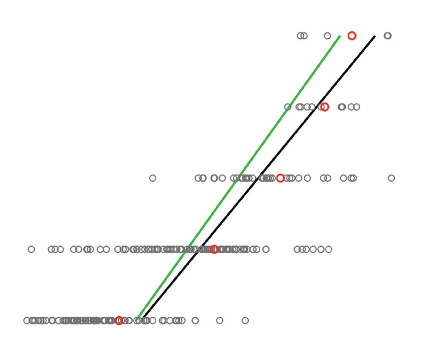
12 Shock and Vibration

 10 10

 9 9

 8 8

 MMI
 MMI

 7 7

 6 6

 5 5

 0.5 1 1.5 2 2.5 3 –0.5 0 0.5 1 1.5 2 2.5
 logPGA logPGV

 Turkey Turkey
 America America
 China China

 (a) (b)

 Figure 9: Distribution of datasets from China, America, and Turkey. (a) MMI versus logPGA. (b) MMI versus logPGV.

 Table 3: Coefficients of equation (1) and standard deviations of residuals for the complete dataset.
PGM c1 c2 σ MMI σ logPGM
PGA 2.906 0.554 0.6069 0.3257
PGV 3.310 3.233 0.6742 0.3280
PSA (0.3 s) 2.873 −0.327 0.6140 0.3390
PSA (1.0 s) 3.065 0.540 0.7027 0.3675
PSA (2.0 s) 4.082 −0.152 1.0265 0.4115
PSA (3.0 s) 4.062 0.817 1.0118 0.3912

 9 9

 8 8
 MMI

 MMI

 7 7

 6 6

 5 5

 1 1.5 2 2.5 3 –0.5 0 0.5 1 1.5 2
 logPGA logPGV

 Regression line Regression line
 Liu et al. [21] Liu et al. [21]
 Data used Data used
 Mean Mean

 (a) (b)

 Figure 10: Regression lines of GMICEs. (a) MMI-logPGA. (b) MMI-logPGV.
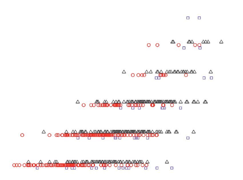
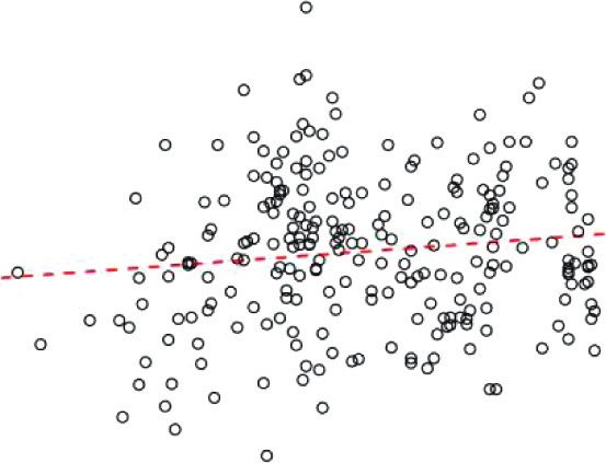
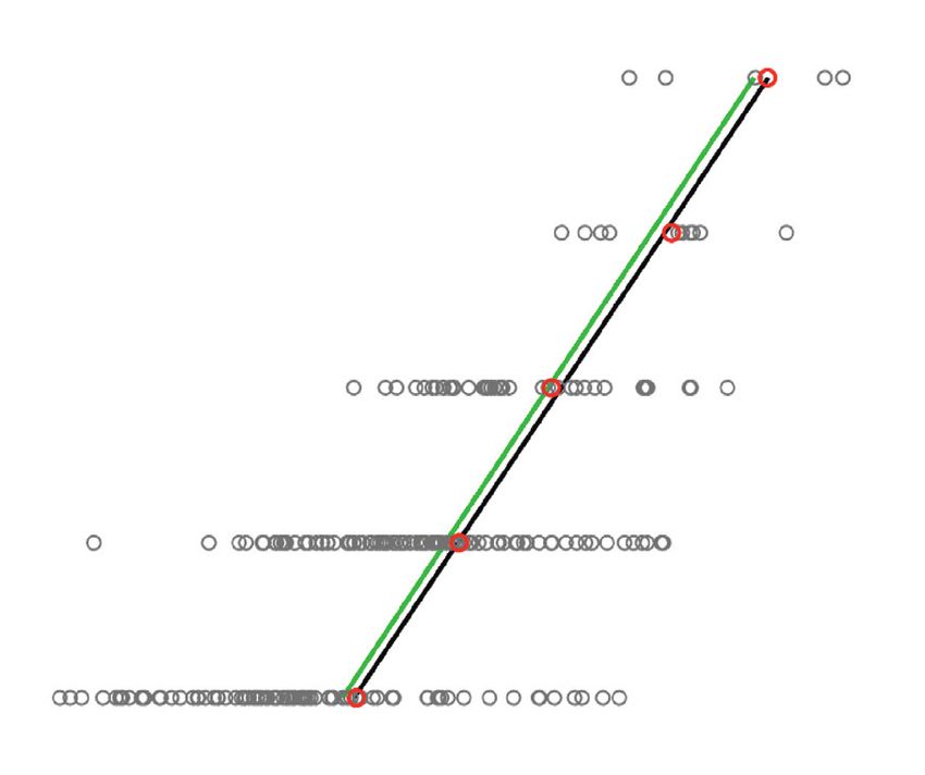
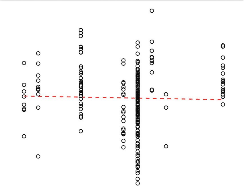
Shock and Vibration 13

 9 9

 8 8
 MMI

 MMI
 7 7

 6 6

 5 5

 0.5 1 1.5 2 2.5 3 3.5 0.5 1 1.5 2 2.5 3
 logPSA (0.3 s) logPSA (1.0 s)

 Regression line Regression line
 Data used Data used
 Mean Mean
 (a) (b)

 9 9

 8 8
 MMI
 MMI

 7 7

 6 6

 5 5

 0 0.5 1 1.5 2 2.5 0 0.5 1 1.5 2 2.5
 logPSA (2.0 s) logPSA (3.0 s)

 Regression line Regression line
 Data used Data used
 Mean Mean
 (c) (d)

Figure 11: Regression lines of GMICEs. (a) MMI-logPSA (0.3 s). (b) MMI-logPSA (1.0 s). (c) MMI-logPSA (2.0 s). (d) MMI-logPSA (3.0 s).

 3
 3
 2
 2

 1 1
 Residuals

 Residuals

 0 0

 –1 –1

 –2
 –2
 –3
 –3
 6 6.5 7 7.5 8 6 6.5 7 7.5 8
 Mw Mw
 Trend line Trend line
 Residual data Residual data
 (a) (b)

 Figure 12: Residuals for MMI predicted from (a) PGA and (b) PGV, as a function of moment magnitude.
14 Shock and Vibration

 3
 3
 2
 2

 1 1
 Residuals

 Residuals
 0 0

 –1 –1

 –2
 –2

 –3
 –3

 1 1.5 2 2.5 3 1 1.5 2 2.5 3
 log R log R
 Trend line Trend line
 Residual data Residual data
 (a) (b)

 Figure 13: Residuals for MMI predicted from (a) PGA and (b) PGV, as a function of the log of hypocentral distance.

 3 3

 2
 2

 1
 1
 Residuals

 Residuals

 0
 0
 –1
 –1
 –2
 –2
 –3
 –3
 5 10 15 20 5 10 15 20
 Hypocentral depth (km) Hypocentral depth (km)
 Trend line Trend line
 Residual data Residual data
 (a) (b)

 Figure 14: Residuals for MMI predicted from (a) PGA and (b) PGV, as a function of hypocentral depth.
Shock and Vibration 15

 3
 3

 2 2
 Residuals
 1 1

 Residuals
 0 0

 –1 –1
 –2 –2
 –3
 –3

 6 6.5 7 7.5 8 6 6.5 7 7.5 8
 Mw Mw
 Trend line Trend line
 Residual data Residual data
 (a) (b)
 5
 5
 4
 4
 3 3
 2 2
 1 1
 Residuals

 Residuals

 0 0
 –1 –1
 –2 –2
 –3
 –3
 –4
 –4
 –5
 –5
 6 6.5 7 7.5 8 6 6.5 7 7.5 8
 Mw Mw
 Trend line Trend line
 Residual data Residual data
 (c) (d)

Figure 15: Residuals for MMI predicted from (a) PSA (0.3 s), (b) PSA (1.0 s), (c) PSA (2.0 s), and (d) PSA (3.0 s), as a function of moment
magnitude.

 3
 3

 2 2

 1 1
 Residuals
 Residuals

 0 0

 –1 –1
 –2 –2
 –3
 –3

 1 1.5 2 2.5 3 1 1.5 2 2.5 3
 log R log R

 Trend line Trend line
 Residual data Residual data
 (a) (b)
 Figure 16: Continued.
16 Shock and Vibration

 5
 5
 4
 4
 3
 3
 2 2
 1

 Residuals
 1
 Residuals

 0 0
 –1 –1
 –2 –2
 –3 –3
 –4 –4
 –5
 –5
 1 1.5 2 2.5 3 1 1.5 2 2.5 3
 log R log R

 Trend line Trend line
 Residual data Residual data
 (c) (d)

Figure 16: Residuals for MMI predicted from (a) PSA (0.3 s), (b) PSA (1.0 s), (c) PSA (2.0 s), and (d) PSA (3.0 s), as a function of the log of
hypocentral distance.

 3 3

 2 2

 1 1
 Residuals

 Residuals

 0 0
 –1 –1
 –2
 –2
 –3
 –3
 5 10 15 20 5 10 15 20
 Hypocentral depth (km) Hypocentral depth (km)

 Trend line Trend line
 Residual data Residual data
 (a) (b)

 5
 4
 4
 3
 3
 2 2
 Residuals

 1
 Residuals

 1
 0 0
 –1 –1
 –2
 –2
 –3
 –3
 –4
 –4
 –5
 5 10 15 20 5 10 15 20
 Hypocentral depth (km) Hypocentral depth (km)

 Trend line Trend line
 Residual data Residual data
 (c) (d)

Figure 17: Residuals for MMI predicted from (a) PSA (0.3 s), (b) PSA (1.0 s), (c) PSA (2.0 s), and (d) PSA (3.0 s), as a function of hypocentral
depth.
Shock and Vibration 17

 Table 4: Coefficients of equation (8) and standard deviations of residuals applying the correction terms.
PGM c3 c4 c5 c6 σ MMI
PGA −0.016 0.523 −0.006 −0.595 0.5698
PGV −0.567 −0.189 0.035 4.529 0.6068
PSA (0.3 s) −0.135 0.467 0.016 0.116 0.5566
PSA (1.0 s) −0.480 −0.287 0.057 3.818 0.6240
PSA (2.0 s) −1.101 −0.473 0.095 8.665 0.8555
PSA (3.0 s) −1.020 −0.594 0.114 8.016 0.8062

 Table 5: GMICEs from the present and previous studies.
 Reference study Proposed equations
 This study I � 2.906 · logPGA + 0.554
 Liu et al. [21] I � 3.333 · logPGA
 Ma et al. [27] I � 2.15 · logPGA + 2.12
 Du et al. [22] I � 3.311 · logPGA − 0.354
 Trifunac and Brady [20] I � 3.333 · logPGA − 0.047

 I � 2.20 · logPGA + 1.00, logPGA ≤ 1.82
 Wald et al. [3]
 I � 3.66 · logPGA − 1.66, logPGA > 1.82
 I � 1.39 · logPGA + 2.65, logPGA ≤ 1.69
MMI-PGA Atkinson and Kaka [5]
 I � 4.09 · logPGA − 1.91, logPGA > 1.69
 Faenza and Michelini [2] I � 2.58 · logPGA + 1.68
 I � 1.55 · logPGA + 1.78, logPGA ≤ 1.57
 Worden et al. [6]
 I � 3.70 · logPGA − 1.60, logPGA > 1.57
 I � 1.647 · logPGA + 2.270, logPGA ≤ 1.6
 Caprio et al. [10]
 I � 3.822 · logPGA − 1.361, logPGA > 1.6
 Ahmadzadeh et al. [12] I � 3.47 · logPGA − 0.58
 I � 1.9920 · logPGA + 1.7601, logPGA < 1.8914
 Mortalla et al. [11]
 I � 3.9322 · logPGA − 1.9095, logPGA ≥ 1.8914
 This study I � 3.310 · logPGV + 3.233
 Liu et al. [21] I � 3.333 · logPGV + 3.333
 Ma et al. [27] I � 2.31 · logPGV + 4.68
 Du et al. [22] I � 3.356 · logPGV + 3.315
 Trifunac and Brady [20] I � 4.000 · logPGV + 2.520
 I � 2.10 · logPGV + 3.40, logPGV ≤ 0.76
 Wald et al. [3]
 I � 3.47 · logPGV + 2.35, logPGV > 0.76
 I � 1.32 · logPGV + 4.37, logPGA ≤ 0.48
 Atkinson and Kaka [5]
 I � 3.03 · logPGV + 3.54, logPGV > 0.48
MMI-PGV
 Faenza and Michelini [2] I � 2.35 · logPGV + 5.11
 I � 1.47 · logPGV + 3.78, logPGV ≤ 0.53
 Worden et al. [6]
 I � 3.16 · logPGV + 2.89, logPGV > 0.53
 I � 1.589 · logPGV + 4.424, logPGV ≤ 0.3
 Caprio et al. [10]
 I � 2.671 · logPGV + 4.018, logPGV > 0.3

 Ahmadzadeh et al. [12] I � 3.31 · logPGV + 3.35

 I � 1.6323 · logPGV + 4.1070, logPGV < 1.0024
 Mortalla et al. [11]
 I � 3.8370 · logPGV + 1.8970, logPGV ≥ 1.0024
18 Shock and Vibration

 Table 5: Continued.
 Reference study Proposed equations
 This study I � 2.873 · logPSA(0.3 s) − 0.327

 Saman et al. [17] I � 5.44 · logPSA(0.3 s) − 5.27
MMI-PSA (0.3 s) I � 1.69 · logPSA(0.3 s) + 1.26, logPSA(0.3 s) ≤ 2.21
 Worden et al. [6]
 I � 4.14 · logPSA(0.3 s) − 4.15, logPSA(0.3 s) > 2.21
 Bilal and Askan [8] I � 3.404 · logPSA(0.3 s) − 0.247
 Panjamani et al. [26] I � 2.846 · logPSA(0.3 s) + 0.045
 This study I � 3.065 · logPSA(1.0 s) + 0.540
 Atkinson and Sonley [28] I � 4 · logPSA(1.0 s) − 2.0
 I � 1.18 · logPSA(1.0 s) + 3.23, logPSA(1.0 s) ≤ 1.50
 Atkinson and Kaka [5]
 I � 2.95 · logPSA(1.0 s) + 0.57, logPSA(1.0 s) > 1.50
MMI-PSA (1.0 s) Saman et al. [17] I � 3.688 · logPSA(1.0 s) − 0.42
 I � 1.51 · logPSA(1.0 s) + 2.50, logPSA(1.0 s) ≤ 1.65
 Worden et al. [6]
 I � 2.90 · logPSA(1.0 s) + 0.20, logPSA(1.0 s) > 1.65
 Bilal and Askan [8] I � 4.119 · logPSA(1.0 s) − 0.934
 Panjamani et al. [26] I � 2.713 · logPSA(1.0 s) + 1.765
 This study I � 4.082 · logPSA(2.0 s) − 0.152
 Saman et al. [17] I � 3.35 · logPSA(2.0 s) + 1.34
MMI-PSA (2.0 s)
 Bilal and Askan [8] I � 4.453 · logPSA(2.0 s) − 0.313
 Panjamani et al. [26] I � 2.152 · logPSA(2.0 s) + 2.713
 This study I � 4.062 · logPSA(3.0 s) + 0.817
MMI-PSA (3.0 s) I � 1.17 · logPSA(3.0 s) + 3.81, logPSA(3.0 s) ≤ 0.99
 Worden et al. [6]
 I � 3.01 · logPSA(3.0 s) + 1.99, logPSA(3.0 s) > 0.99
 Panjamani et al. [26] I � 2.447 · logPSA(3.0 s) + 3.589

 12 12
 11 11
 10 10
 9 9
 8 8
 7 7
 MMI

 MMI

 6 6
 5 5
 4 4
 3 3
 2 2
 1 1

 –1 –0.5 0 0.5 1 1.5 2 2.5 3 3.5 4 –2 –1.5 –1 –0.5 0 0.5 1 1.5 2 2.5
 logPGA logPGV

 This study Faenza and Michelini [2] This study Faenza and Michelini [2]
 Liu et al. [21] Worden et al. [6] Liu et al. [21] Worden et al. [6]
 Ma et al. [27] Caprio et al. [10] Ma et al. [27] Caprio et al. [10]
 Du et al. [22] Ahmadzadeh et al. [12] Du et al. [22] Ahmadzadeh et al. [12]
 Trifunac and Brady [20] Mortalla et al. [11] Trifunac and Brady [20] Mortalla et al. [11]
 Wald et al. [3] Data used Wald et al. [3] Data used
 Atkinson and Kaka [5] Atkinson and Kaka [5]

 (a) (b)

Figure 18: Comparison of GMICEs obtained in this study with similar equations from previous studies. (a) MMI-PGA. (b) MMI-PGV.
Shock and Vibration 19

 10 10
 9 9
 8 8
 7 7
 6 6
 MMI

 MMI
 5 5
 4 4
 3 3
 2 2
 1 1

 0 0.5 1 1.5 2 2.5 3 3.5 –1 –0.5 0 0.5 1 1.5 2 2.5 3
 logPSA (0.3s) logPSA (1.0 s)

 This study This study
 Saman et al. [17] Atkinson and Sonley [28]
 Worden et al. [6] Atkinson and Kaka [5]
 Bilal and Askan [8] Saman et al. [17]
 Panjamani et al. [26] Worden et al. [6]
 Data used Bilal and Askan [8]
 Panjamani et al. [26]
 Data used
 (a) (b)

 10 10
 9 9
 8 8
 7 7
 6 6
 MMI

 MMI

 5 5
 4 4
 3 3
 2 2
 1 1

 –0.5 0 0.5 1 1.5 2 2.5 3 –1.5 –1 –0.5 0 0.5 1 1.5 2 2.5
 logPSA (2.0 s) logPSA (3.0 s)

 This study This study
 Saman et al. [17] Worden et al. [6]
 Bilal and Askan [8] Panjamani et al. [26]
 Panjamani et al. [26] Data used
 Data used
 (c) (d)

Figure 19: Comparison of GMICEs obtained in this study with similar equations from previous studies. (a) MMI-PSA (0.3 s). (b) MMI-PSA
(1.0 s). (c) MMI-PSA (2.0 s). (d) MMI-PSA (3.0 s).

for PSA at present, we cannot get the regional correction elect to employ orthogonal regression and obtain the re-
factor of PSA for China in our study. versible relationships, which provide a stable conversion
 from ground motion to MMI or MMI to ground motion. It
7. Conclusion is believed that these new GMICEs proposed herein can be
 used in the future whenever necessary in China, particularly
In this study, we use the strong motion records and seismic for preparing intensity maps, earthquake disaster and loss
intensity data from 11 moderate-to-strong earthquakes in assessment, and other engineering applications.
the mainland of China since 2008 and develop new con- We analyze the effects of the moment magnitude, hypo-
version equations between MMI and PGA, PGV, PSA (0.3 s), central distance, and hypocentral depth on the residuals of
PSA (1.0 s), PSA (2.0 s), and PSA (3.0 s). Unlike earlier conversion equations. By introducing a magnitude-distance-
studies in China (e.g., Liu et al. [21] and Ma et al. [27]), we depth correction term, we obtain the improved relationships
20 Shock and Vibration

and remove the trends in residuals. It should be noted that application in ShakeMap,” Geophysical Journal International,
Vs30, a factor characterizing the site conditions at the locations vol. 180, no. 3, pp. 1138–1152, 2010.
of interest, is also a potential independent variable in the [3] D. J. Wald, V. Quitoriano, T. H. Heaton, and H. Kanamori,
conversion equations. However, as of now, there are numerous “Relationships between peak ground acceleration, peak
strong motion stations in China without detailed information ground velocity, and modified Mercalli intensity in Cal-
on local site conditions. Therefore, we do not include a site ifornia,” Earthquake Spectra, vol. 15, no. 3, pp. 557–564, 1999.
 [4] S. I. Kaka and G. M. Atkinson, “Relationships between in-
correction term in our improved conversion relationships.
 strumental ground-motion parameters and modified Mercalli
 The proposed conversion equations are also compared with
 intensity in eastern North America,” Bulletin of the Seismo-
similar relationships from previous studies. These comparisons logical Society of America, vol. 94, no. 5, pp. 1728–1736, 2004.
confirm that such relationships should be regionally depen- [5] G. M. Atkinson and S. I. Kaka, “Relationships between felt
dent. Since the limited dataset used in this study mainly comes intensity and instrumental ground motion in the central
from the central and western regions of China, the conclusions United States and California,” Bulletin of the Seismological
in this paper are only applicable to these regions. An alternative Society of America, vol. 97, no. 2, pp. 497–510, 2007.
approach is also proposed with a regional correction factor for [6] C. B. Worden, M. C. Gerstenberger, D. A. Rhoades, and
China, suitable for the global relationships proposed by Caprio D. J. Wald, “Probabilistic relationships between ground-
et al. [10]. This makes the regional characteristics of China motion parameters and modified Mercalli intensity in Cal-
comparable to other regions in the globe having the global ifornia,” Bulletin of the Seismological Society of America,
relationships as reference. vol. 102, no. 1, pp. 204–221, 2012.
 It is also worth noting that the GMICEs in the present [7] V. Y. Sokolov, “Seismic intensity and Fourier acceleration
study should not be used beyond the PGM and MMI ranges spectra: revised relationship,” Earthquake Spectra, vol. 18,
indicated in Tables 1 and 2 (MMI range between V to IX, Mw no. 1, pp. 161–187, 2002.
 [8] M. Bilal and A. Askan, “Relationships between felt intensity
range between 5.9 and 7.9, and hypocentral distance range
 and recorded ground-motion parameters for Turkey,” Bul-
covering 11.2–640.5 km), and PGM data used to develop the
 letin of the Seismological Society of America, vol. 104, no. 1,
equations correspond to the maximum of the two horizontal pp. 484–496, 2014.
components. In the future, similar studies need to be [9] Y.-M. Wu, T. L. Teng, T. C. Shin, and N. C. Hsiao, “Rela-
conducted with more seismic records and intensity data to tionship between peak ground acceleration, peak ground
further optimize and improve the GMICEs for China. velocity, and intensity in Taiwan,” Bulletin of the Seismological
 Society of America, vol. 93, no. 1, pp. 386–396, 2003.
Data Availability [10] M. Caprio, B. Tarigan, C. B. Worden, S. Wiemer, and
 D. J. Wald, “Ground motion to intensity conversion equations
The strong motion records used in this study were provided (GMICEs): a global relationship and evaluation of regional
by the China Strong Motion Network Center. The macro- dependency,” Bulletin of the Seismological Society of America,
seismic intensity dataset, including the intensity maps and vol. 105, no. 12, pp. 1–21, 2015.
post-earthquake disaster investigation reports, was acquired [11] J. M. Mortalla, T. Godes, D. A. Rhoades, S. Canessa, and
 M. C. Gerstenberger, “New ground motion to intensity
from the provincial seismological bureaus operating under
 conversion equations (GMICEs) for New Zealand,” Seismo-
the China Earthquake Administration.
 logical Research Letters, vol. 92, no. 1, pp. 448–459, 2021.
 [12] S. Ahmadzadeh, G. J. Doloei, and H. Zafarani, “Ground
Conflicts of Interest motion to intensity conversion equations for Iran,” Pure and
 Applied Geophysics, vol. 177, no. 11, pp. 5435–5449, 2020.
The authors declare that they have no conflicts of interest. [13] B. Gutenberg and C. F. Richter, “Earthquake magnitude,
 intensity, energy, and acceleration,” Bulletin of the Seismo-
Acknowledgments logical Society of America, vol. 46, no. 2, pp. 105–145, 1956.
 [14] J. Hershberger, “A comparison of earthquake accelerations
This study was supported by Basic Scientific Research Fund with intensity ratings∗ ,” Bulletin of the Seismological Society of
of Science and Technology Innovation Base of Lanzhou, America, vol. 46, no. 4, pp. 317–320, 1956.
Institute of Earthquake Forecasting, China Earthquake [15] E. L. Krinitzsky and F. K. Chang, “Intensity-related earth-
 quake ground motions,” Environmental and Engineering
Administration (grant no. 2019IESLZ06). The authors would
 Geoscience, vol. xxv, no. 4, pp. 425–435, 1988.
like to thank the China Strong Motion Network Center for [16] G. F. Panza, F. Vaccari, and R. Cazzaro, “Correlation between
providing strong motion records and the provincial seis- macroseismic intensities and seismic ground motion pa-
mological bureaus operating under the China Earthquake rameters,” Annali di Geofisica, vol. 15, pp. 1371–1382, 1997.
Administration for providing the isoseismal maps and [17] Y. S. Saman, H. H. Tsang, and T. K. L. Nelson, “Conversion
damage reports of the past earthquakes. between peak ground motion parameters and modified
 Mercalli intensity Values,” Journal of Earthquake Engineering,
References vol. 15, pp. 1138–1155, 2011.
 [18] R. Spence, A. Coburn, and A. Pomonis, “Correlation of
 [1] Y. X. Hu, Earthquake Engineering, Seismological Press, Bei- ground motion with building damage: the definition of a new
 jing, China, 2006. damage-based seismic intensity scale,” in Proceedings of the
 [2] L. Faenza and A. Michelini, “Regression analysis of MCS Tenth World Conference on Earthquake Engineering, vol. 1,
 intensity and ground motion parameters in Italy and its pp. 551–556, Madrid, Spain, July 1992.
Shock and Vibration 21

[19] J. Boatwright, K. Thywissen, and L. C. Seekins, “Correlation of
 ground motion and intensity for the 17 January 1994
 Northridge, California, earthquake,” Bulletin of the Seismo-
 logical Society of America, vol. 91, no. 4, pp. 739–752, 2001.
[20] M. D. Trifunac and A. G. Brady, “On the correlation of seismic
 intensity scales with the peaks of recorded strong ground
 motion,” Bulletin of the Seismological Society of America,
 vol. 65, no. 1, pp. 139–162, 1975.
[21] H. X. Liu, R. Lu, and D. Chen, “A proposal of revised china’s
 seismic intensity,” The Selection Of Earthquake Engineering
 Paper From Huixian Liu, Institute of Engineering Mechanics,
 China Earthquake Administration, Harbin, China, 1980.
[22] K. Du, B. Ding, H. Luo, and J. Sun, “Relationship between
 peak ground acceleration, peak ground velocity, and mac-
 roseismic intensity in western China,” Bulletin of the Seis-
 mological Society of America, vol. 109, no. 1, pp. 284–297,
 2018.
[23] H. Y. Yu, B. F. Zhou, W. X. Jiang et al., “Data processing and
 preliminary analysis of strong motion records from the Ms7.0
 Lushan, China earthquake,” Applied Mechanics and Materials,
 vol. 580-583, pp. 1528–1532, 2014.
[24] H. Y. Yu, W. X. Ding, M. Chen et al., Statistical Interpretation
 of Data: Detection and Treatment of Outliers in the Normal
 Sample (GB/T4883-2008), Standards Press of China, Beijing,
 China, 2008.
[25] W. E. Deming, Statistical Adjustment of Data, Wiley, New-
 york, America, 1943.
[26] A. Panjamani, K. Bajaj, S. S. R. Moustafa, and N. S. N. Al-Arifi,
 “Relationship between intensity and recorded ground-motion
 and spectral parameters for the himalayan region,” Bulletin of
 the Seismological Society of America, vol. 106, no. 4,
 pp. 1672–1689, 2016.
[27] Q. Ma, S. L. Li, S. Y. Li, and D. W. Tao, “The correlation of
 ground motion parameters with seismic intensity,” Earth-
 quake Engineering and Engineering Dynamics, vol. 34, no. 4,
 pp. 83–92, 2014.
[28] G. M. Atkinson and E. Sonley, “Empirical relationships be-
 tween modified Mercalli intensity and response spectra,”
 Bulletin of the Seismological Society of America, vol. 90, no. 2,
 pp. 537–544, 2000.
You can also read