News article segmentation using multimodal input - Using Mask R-CNN and sentence transformers - kth .diva
←
→
Page content transcription
If your browser does not render page correctly, please read the page content below

Examensarbete inom datalogi och datateknik, avancerad nivå, 30 hp
       Degree project in computer science, second level

       News article segmentation using
       multimodal input
       Using Mask R-CNN and sentence transformers

       GUSTAV HENNING

Stockholm, Sverige 2022
News article segmentation
using multimodal input

Using Mask R-CNN and sentence
transformers

GUSTAV HENNING

Degree Programme in Computer Science and Engineering
Date: February 11, 2022

Supervisor: Jakob Nyberg
Examiner: Aristides Gionis
   School of Electrical Engineering and Computer Science
Host organization: National Library of Sweden, Kungliga Biblioteket
Swedish title: Artikelsegmentering med multimodala artificiella
neuronnätverk
Swedish subtitle: Med hjälp av Mask R-CNN och sentence
transformers

© 2022 Gustav Henning

Abstract | i

Abstract
In this century and the last, serious efforts have been made to digitize the
content housed by libraries across the world. In order to open up these
volumes to content-based information retrieval, independent elements such as
headlines, body text, bylines, images and captions ideally need to be connected
semantically as article-level units. To query on facets such as author, section,
content type or other metadata, further processing of these documents is
required.
    Even though humans have shown exceptional ability to segment different
types of elements into related components, even in languages foreign to
them, this task has proven difficult for computers. The challenge of semantic
segmentation in newspapers lies in the diversity of the medium: Newspapers
have vastly different layouts, covering diverse content, from news articles to
ads to weather reports.
    State-of-the-art object detection and segmentation models have been
trained to detect and segment real-world objects. It is not clear whether these
architectures can perform equally well when applied to scanned images of
printed text. In the domain of newspapers, in addition to the images themselves,
we have access to textual information through Optical Character Recognition.
    The recent progress made in the field of instance segmentation of real-
world objects using deep learning techniques begs the question: Can the same
methodology be applied in the domain of newspaper articles?
    In this thesis we investigate one possible approach to encode the textual
signal into the image in an attempt to improve performance.
    Based on newspapers from the National Library of Sweden, we investigate
the predictive power of visual and textual features and their capacity to
generalize across different typographic designs. Results show impressive mean
Average Precision scores (>0.9) for test sets sampled from the same newspaper
designs as the training data when using only the image modality.

Keywords
Historical newspapers, Image segmentation, Multimodal learning, Deep
learning, Digital humanities, Mask R-CNN
ii | Abstract

Sammanfattning | iii

Sammanfattning
I detta och det förra århundradet har kraftiga åtaganden gjorts för att digitalisera
traditionellt medieinnehåll som tidigare endast tryckts i pappersformat. För
att kunna stödja sökningar och fasetter i detta innehåll krävs bearbetning
påsemantisk nivå, det vill säga att innehållet styckas upp påartikelnivå, istället
för per sida. Trots att människor har lätt att dela upp innehåll påsemantisk nivå,
även påett främmande språk, fortsätter arbetet för automatisering av denna
uppgift.
     Utmaningen i att segmentera nyhetsartiklar återfinns i mångfalden av
utseende och format. Innehållet är även detta mångfaldigt, där man återfinner
allt ifrån faktamässiga artiklar, till debatter, listor av fakta och upplysningar,
reklam och väder bland annat. Stora framsteg har gjorts inom djupinlärning just
för objektdetektering och semantisk segmentering bara de senaste årtiondet.
Frågan vi ställer oss är: Kan samma metodik appliceras inom domänen
nyhetsartiklar?
     Dessa modeller är skapta för att klassificera världsliga ting. I denna domän
har vi tillgång till texten och dess koordinater via en potentiellt bristfällig optisk
teckenigenkänning. Vi undersöker ett sätt att utnyttja denna textinformation
i ett försök att förbättra resultatet i denna specifika domän. Baserat pådata
från Kungliga Biblioteket undersöker vi hur väl denna metod lämpar sig
för uppstyckandet av innehåll i tidningar längsmed tidsperioder där designen
förändrar sig markant. Resultaten visar att Mask R-CNN lämpar sig väl för
användning inom domänen nyhetsartikelsegmentering, även utan texten som
input till modellen.

Nyckelord
Historiska tidningar, Bildsegmentering, Multimodal inlärning, Djupinlärning,
Digital humaniora, Mask R-CNN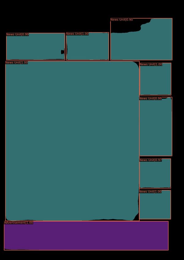
iv | Sammanfattning
Acknowledgments | v

Acknowledgments
In this section, I would like to acknowledge the people who have encouraged,
influenced, helped and supported me during the duration of this study. I would
like to start by thanking and acknowledging my examiner Aristides Gionis and
my supervisor Jakob Nyberg, for their guidance and interest shown throughout
the project, as well as their invaluable feedback.
    I would also like to thank Kungliga Biblioteket, especially Faton Rekathati
and Chris Haffenden, for their encouragement, interest in the topic, and
invaluable help across the timeline of the project.
    This work would not have been possible without the long and arduous
path behind me. To my friends and family who have relentlessly supported me
throughout my life: Thank you.
    And to the scientists before me: Because of you, we stand on the shoulders
of giants. The curious quest to understand the nature of reality continues.

    "I don’t feel frightened by not knowing things. I think it’s much more
interesting."
    - Richard Feynman

Stockholm, February 2022
Gustav Henning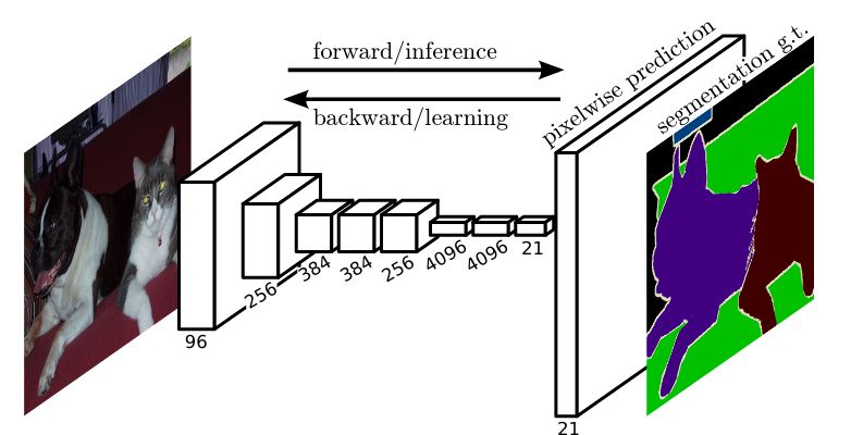
vi | Acknowledgments
Contents | vii

Contents

1   Introduction                                                                                              1
    1.1 Background and problem context        .   .   .   .   .   .   .   .   .   .   .   .   .   .   .   .   1
    1.2 Problem . . . . . . . . . . . . .     .   .   .   .   .   .   .   .   .   .   .   .   .   .   .   .   2
    1.3 Purpose . . . . . . . . . . . . .     .   .   .   .   .   .   .   .   .   .   .   .   .   .   .   .   2
    1.4 Goals . . . . . . . . . . . . . .     .   .   .   .   .   .   .   .   .   .   .   .   .   .   .   .   2
    1.5 Research Methodology . . . . .        .   .   .   .   .   .   .   .   .   .   .   .   .   .   .   .   3
    1.6 Delimitations . . . . . . . . . .     .   .   .   .   .   .   .   .   .   .   .   .   .   .   .   .   3
    1.7 Ethical considerations . . . . . .    .   .   .   .   .   .   .   .   .   .   .   .   .   .   .   .   4
    1.8 Structure of the thesis . . . . . .   .   .   .   .   .   .   .   .   .   .   .   .   .   .   .   .   4

2   Background                                                                                                 5
    2.1 Data . . . . . . . . . . . . . . . . . . . . . . . . . . .                            .   .   .   .    5
        2.1.1 Digitization of historical documents . . . . . .                                .   .   .   .    5
        2.1.2 Digitization at the National Library of Sweden                                  .   .   .   .    6
        2.1.3 Description . . . . . . . . . . . . . . . . . . .                               .   .   .   .    6
                2.1.3.1 Summary pages . . . . . . . . . . .                                   .   .   .   .    6
                2.1.3.2 Content pages . . . . . . . . . . . .                                 .   .   .   .    7
                2.1.3.3 Listings . . . . . . . . . . . . . . .                                .   .   .   .    7
                2.1.3.4 Comics, artwork and poems . . . . .                                   .   .   .   .    7
                2.1.3.5 Games, puzzles and quizzes . . . . .                                  .   .   .   .    7
                2.1.3.6 Weather . . . . . . . . . . . . . . .                                 .   .   .   .    7
    2.2 Deep learning preliminaries . . . . . . . . . . . . . .                               .   .   .   .    8
        2.2.1 Convolutional Neural Network . . . . . . . . .                                  .   .   .   .    8
        2.2.2 Fully Convolutional Network . . . . . . . . . .                                 .   .   .   .   11
        2.2.3 Feature Pyramid Network . . . . . . . . . . .                                   .   .   .   .   12
        2.2.4 Mask R-CNN . . . . . . . . . . . . . . . . . .                                  .   .   .   .   13
        2.2.5 Microsoft COCO: Common Objects in Context                                       .   .   .   .   15
    2.3 Related work . . . . . . . . . . . . . . . . . . . . . .                              .   .   .   .   15
        2.3.1 Segmentation Algorithms . . . . . . . . . . .                                   .   .   .   .   15
viii | Contents
2.3.1.1 Classical Approaches . . . . . . . . . . . . 16
2.3.1.2 Deep Learning Approaches . . . . . . . . . 17
2.3.2 Word representation language models . . . . . . . . . 18
2.3.2.1 From classical methods to state-of-the-art . 19
2.3.2.2 BERT . . . . . . . . . . . . . . . . . . . . 21
2.3.2.3 Sentence-BERT . . . . . . . . . . . . . . . 21
2.4 Metrics . . . . . . . . . . . . . . . . . . . . . . . . . . . . . 22
2.4.1 Mean Intersection over Union . . . . . . . . . . . . . 22
2.4.2 Precision and Recall . . . . . . . . . . . . . . . . . . 22
2.4.3 Mean Average Precision . . . . . . . . . . . . . . . . 23
3 Method 25
3.1 Data . . . . . . . . . . . . . . . . . . . . . . . . . . . . . . . 25
3.1.1 Data Sampling . . . . . . . . . . . . . . . . . . . . . 25
3.1.1.1 Domain-related datasets . . . . . . . . . . . 26
3.1.1.2 DN 2010 - 2020 (In-set) . . . . . . . . . . . 26
3.1.1.3 DN SvD 2001 - 2004 (Near-set) . . . . . . . 27
3.1.1.4 Aftonbladet Expressen 2001 - 2004 (Out-set) 27
3.1.2 Labeling strategy . . . . . . . . . . . . . . . . . . . . 27
3.1.2.1 Static content . . . . . . . . . . . . . . . . 28
3.1.2.2 Overlapping labels . . . . . . . . . . . . . . 28
3.1.2.3 Extending labels . . . . . . . . . . . . . . . 28
3.1.2.4 Blocking labels . . . . . . . . . . . . . . . 29
3.1.2.5 Caveats of processing individual pages . . . 30
3.1.3 Labels . . . . . . . . . . . . . . . . . . . . . . . . . . 30
3.1.3.1 Final classes . . . . . . . . . . . . . . . . . 31
3.1.3.2 Background . . . . . . . . . . . . . . . . . 31
3.1.3.3 News Unit . . . . . . . . . . . . . . . . . . 31
3.1.3.4 News Unit Delimitations . . . . . . . . . . 32
3.1.3.5 Advertisement . . . . . . . . . . . . . . . . 32
3.1.3.6 Listing . . . . . . . . . . . . . . . . . . . . 33
3.1.3.7 Weather . . . . . . . . . . . . . . . . . . . 33
3.1.3.8 Death Notice . . . . . . . . . . . . . . . . . 34
3.1.3.9 Game . . . . . . . . . . . . . . . . . . . . . 34
3.1.3.10 Publication Unit . . . . . . . . . . . . . . . 34
3.1.3.11 Delimitations . . . . . . . . . . . . . . . . 35
3.2 Model Architecture . . . . . . . . . . . . . . . . . . . . . . . 36
3.2.1 Primary architecture . . . . . . . . . . . . . . . . . . 36
3.2.1.1 Preprocessing . . . . . . . . . . . . . . . . 37Contents | ix
3.2.2 Modifications to the primary architecture . . . . . . . 38
3.2.2.1 Multiscale training . . . . . . . . . . . . . . 40
3.2.2.2 Optimizer . . . . . . . . . . . . . . . . . . 40
3.2.3 Text Embedding map . . . . . . . . . . . . . . . . . . 40
3.2.3.1 Text embedding strategy . . . . . . . . . . . 45
3.2.3.2 Sentence transformers . . . . . . . . . . . . 45
3.3 Experiments . . . . . . . . . . . . . . . . . . . . . . . . . . . 46
3.3.1 Unimodal versus multimodal input . . . . . . . . . . . 46
3.3.2 Impact of class labels . . . . . . . . . . . . . . . . . . 46
3.3.3 Impact of dataset size . . . . . . . . . . . . . . . . . . 46
3.4 System documentation . . . . . . . . . . . . . . . . . . . . . 47
3.4.1 Hardware specifications . . . . . . . . . . . . . . . . 47
3.4.2 Software specifications . . . . . . . . . . . . . . . . . 47
3.4.2.1 MMDetection . . . . . . . . . . . . . . . . 47
3.4.2.2 Label studio . . . . . . . . . . . . . . . . . 47
3.4.2.3 Software versions . . . . . . . . . . . . . . 47
4 Results 49
4.1 Unimodal versus multimodal . . . . . . . . . . . . . . . . . . 50
4.1.1 6 classes . . . . . . . . . . . . . . . . . . . . . . . . 51
4.1.2 1 class . . . . . . . . . . . . . . . . . . . . . . . . . . 52
4.2 Impact of dataset size . . . . . . . . . . . . . . . . . . . . . . 53
4.2.1 6 classes . . . . . . . . . . . . . . . . . . . . . . . . 53
4.2.2 1 class . . . . . . . . . . . . . . . . . . . . . . . . . . 54
4.3 Impact of classes . . . . . . . . . . . . . . . . . . . . . . . . 55
4.4 Visual examples . . . . . . . . . . . . . . . . . . . . . . . . . 58
5 Discussion 65
5.1 Labeling strategy and choices of classes . . . . . . . . . . . . 65
5.1.1 Borderline cases in labeling . . . . . . . . . . . . . . 66
5.1.1.1 Advertisement . . . . . . . . . . . . . . . . 66
5.1.1.2 Listings . . . . . . . . . . . . . . . . . . . 66
5.1.2 Results of class impact . . . . . . . . . . . . . . . . . 66
5.2 Mask R-CNN . . . . . . . . . . . . . . . . . . . . . . . . . . 67
5.2.1 Higher performance is required for usefulness within
the domain of newspaper article segmentation . . . . . 67
5.2.2 Unaltered Mask R-CNN performs well on in-domain
datasets . . . . . . . . . . . . . . . . . . . . . . . . . 67
5.3 Sentence transformers . . . . . . . . . . . . . . . . . . . . . . 67x | Contents
5.3.1 Large text embeddings . . . . . . . . . . . . . . . . . 67
5.4 Impact of dataset size . . . . . . . . . . . . . . . . . . . . . . 68
5.5 Combining other methods . . . . . . . . . . . . . . . . . . . . 68
6 Conclusions and Future Work 69
6.1 Conclusions . . . . . . . . . . . . . . . . . . . . . . . . . . . 69
6.2 Limitations . . . . . . . . . . . . . . . . . . . . . . . . . . . 70
6.3 Future work . . . . . . . . . . . . . . . . . . . . . . . . . . . 70
References 73
.1 Appendix A: Definitions related to news articles . . . . . . . . 77List of Figures | xi
List of Figures
2.1 Movement of the kernel within the input image or filter matrix [5]. 9
2.2 Zero-padding [5]. . . . . . . . . . . . . . . . . . . . . . . . . 10
2.3 Residual block [6]. . . . . . . . . . . . . . . . . . . . . . . . 11
2.4 Fully Convolutional Network architecture as depicted in the
original paper [7]. . . . . . . . . . . . . . . . . . . . . . . . . 11
2.5 Evolution of the Feature Pyramid Network [8]. . . . . . . . . . 13
2.6 Mask R-CNN results on the MS COCO dataset [12]. Masks
are shown in color. Bounding boxes, category and confidence
are also shown. . . . . . . . . . . . . . . . . . . . . . . . . . 15
2.7 Hierarchical typology of document segmentation algorithms [2].
. . . . . . . . . . . . . . . . . . . . . . . . . . . . . . . . . 17
3.1 Asymmetric extension of the label. A is labeled red, and B
should belong to the same label, while C should not. . . . . . 29
3.2 Example where other content (C) is blocking elements (A and
B) from becoming one label. . . . . . . . . . . . . . . . . . . 30
3.3 Ground truth label comparison between labels for 6 classes
versus labels using the Publication Unit superclass. Both
figures a) and b) depict the labels of the same newspaper image,
an image from the DN 2010-2020 Test subset (Section 3.1.1.2). 35
3.4 Left: A block of ResNet. Right: A block of ResNeXt with
cardinality = 32. [37] . . . . . . . . . . . . . . . . . . . . . . 37
3.5 Left: Aggregating transformations of depth = 2 Right: An
equivalent block, which is trivially wider. [37] . . . . . . . . . 37
3.6 Distribution of annotations by squareroot area. . . . . . . . . 39
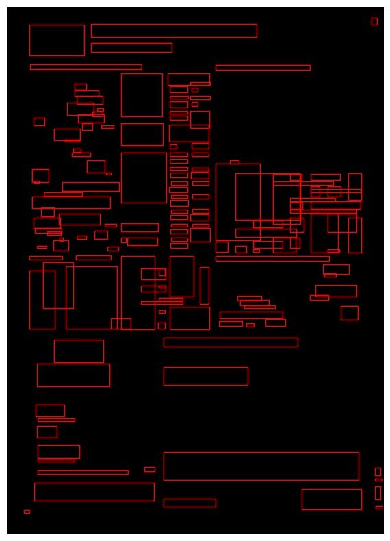
3.7 A front page newspaper page from the DN 2010-2020 Test
subset. *In (b) the first 3 dimensions of "all-mpnet-base-v2"
vector representations normalized as RGB colors. . . . . . . . 42xii | List of Figures
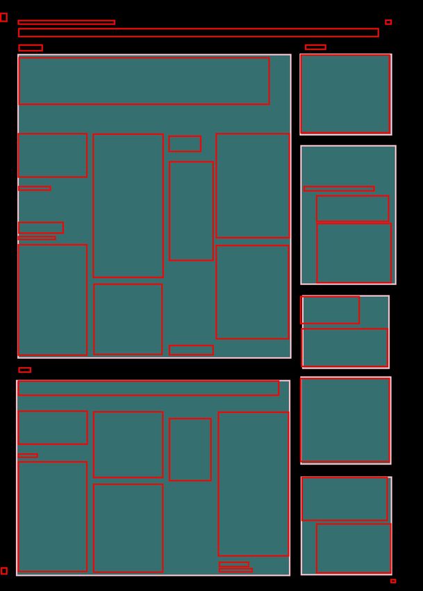
3.8 A newspaper page with obituaries from the DN 2010-2020 Test
subset. *In (b) the first 3 dimensions of "all-mpnet-base-v2"
vector representations normalized as RGB colors. . . . . . . . 43
3.9 A newspaper page with news articles from the DN 2010-2020
Test subset. *In (b) the first 3 dimensions of "all-mpnet-base-
v2" vector representations normalized as RGB colors. . . . . . 44
4.1 Normalized confusion matrices for the one class experiment
on the In-domain test set found in Table 4.11. Percentages are
rounded down. . . . . . . . . . . . . . . . . . . . . . . . . . 55
4.2 Normalized confusion matrix for r50 Mask R-CNN 75%. See
Table 4.8. Percentages are rounded down. . . . . . . . . . . . 56
4.3 Normalized confusion matrix for r50 Mask R-CNN 100%. See
Table 4.8. Percentages are rounded down. . . . . . . . . . . . 57
4.4 A front page newspaper page from the DN 2010-2020 Test
subset. In subfigures (b), (c) and (d) the teal labels are News
units, and the purple is Advertisement. . . . . . . . . . . . . . 59
4.5 A newspaper page with listing prices of funds and stocks from
the DN 2010-2020 Test subset. In subfigures (b), (c) and (d)
the bright purple label is Advertisement, and the dark purple
labels are Listings. . . . . . . . . . . . . . . . . . . . . . . . 60
4.6 A newspaper page with obituaries from the DN 2010-2020 Test
subset. In subfigures (b), (c) and (d) the bright green labels are
Death Notice (obituaries). . . . . . . . . . . . . . . . . . . . . 61
4.7 A newspaper page consisting of news articles from the DN
2010-2020 Test subset. In subfigures (b), (c) and (d) the teal
labels are News Units. . . . . . . . . . . . . . . . . . . . . . . 62
4.8 A newspaper page consisting of weather reports and advertise-
ment from the DN 2010-2020 Test subset. In subfigures (b), (c)
and (d) the blue label is Weather. Purple labels are Advertisement. 63
4.9 A newspaper page consisting of a single large image, part of
a multi-page article from the DN 2010-2020 Test subset. In
subfigures (b), (c) and (d) the teal label is News unit. . . . . . 64List of Tables | xiii
List of Tables
3.1 Annotated pages in the datasets . . . . . . . . . . . . . . . . . 26
3.2 Class distribution in the DN 2010 - 2020 dataset . . . . . . . . 27
3.3 Class distribution in the DN SvD 2001 - 2004 dataset . . . . . 27
3.4 Class distribution in the Aftonbladet Expressen 2001 - 2004
dataset . . . . . . . . . . . . . . . . . . . . . . . . . . . . . . 27
3.5 Object size threshold differences in pixels . . . . . . . . . . . 39
3.6 Number of annotations per area group for the test sets . . . . . 39
3.7 Sentence transformers . . . . . . . . . . . . . . . . . . . . . . 45
3.8 Class distribution in partial datasets of DN 2010 - 2020 (In-set) 46
3.9 Hardware specifications . . . . . . . . . . . . . . . . . . . . . 47
3.10 Software versions . . . . . . . . . . . . . . . . . . . . . . . . 48
4.1 Model names . . . . . . . . . . . . . . . . . . . . . . . . . . 50
4.2 Top 5 results - 6 classes - In-set (Section 3.1.1.2) . . . . . . . 51
4.3 Top 5 results - 6 classes - Near-set (Section 3.1.1.3) . . . . . . 51
4.4 Top 5 results - 6 classes - Out-set (Section 3.1.1.4) . . . . . . . 51
4.5 Top 5 results - 1 class - In-set (Section 3.1.1.2) . . . . . . . . . 52
4.6 Top 5 results - 1 class - Near-set (Section 3.1.1.3) . . . . . . . 52
4.7 Top 5 results - 1 class - Out-set (Section 3.1.1.4) . . . . . . . . 52
4.8 Gradually increasing dataset size - 6 classes - In-set (Sec-
tion 3.1.1.2) . . . . . . . . . . . . . . . . . . . . . . . . . . . 53
4.9 Gradually increasing dataset size - 6 classes - Near-set
(Section 3.1.1.3) . . . . . . . . . . . . . . . . . . . . . . . . . 53
4.10 Gradually increasing dataset size - 6 classes - Out-set
(Section 3.1.1.4) . . . . . . . . . . . . . . . . . . . . . . . . . 53
4.11 Gradually increasing dataset size - 1 class - In-set (Sec-
tion 3.1.1.2) . . . . . . . . . . . . . . . . . . . . . . . . . . . 54
4.12 Gradually increasing dataset size - 1 class - Near-set
(Section 3.1.1.3) . . . . . . . . . . . . . . . . . . . . . . . . . 54xiv | List of Tables
4.13 Gradually increasing dataset size - 1 class - Out-set (Sec-
tion 3.1.1.4) . . . . . . . . . . . . . . . . . . . . . . . . . . . 54List of acronyms and abbreviations | xv List of acronyms and abbreviations ANN Artificial Neural Network BERT Bidirectional Encoder Representations from Transformers BoW Bag of Words CBOW Continuous Bag of Words CNN Convolutional Neural Network COCO Common Objects in Context DN Dagens Nyheter DNN Deep Neural Network FCN Fully Convolutional (Neural) Network FN False Negative FP False Positive FPN Feature Pyramid Network GloVe Global Vectors GPU Graphical Processing Unit IoU Intersection over Union mAP mean Average Precision mIoU mean Interesection over Union NLP Natural Language Processing OCR Optical Character Recognition
xvi | List of acronyms and abbreviations

R-CNN Region Based Convolutional Neural Network

ResNet Residual Neural Network

RGB Red Green Blue

RLSA Run-Length Smoothing Algorithm

RoI Region of Interest

RPN Region Proposal Network

SBERT Sentence-BERT

SVD Svenska Dagbladet

TF Term Frequency

TF-IDF Term Frequency-Inverse Document Frequency

TN True Negative

TP True Positive
Introduction | 1

Chapter 1

Introduction

Nowadays it is commonplace for memory institutions to create and maintain
large digital repositories that offer rapid, time- and location-independent access
to documents. This is the culmination of a continuous digitization effort
spanning several decades of achievements in preservation and accessibility.
Another promise of digitization, aside from the aspect of access, are the benefits
of exploration support gained by processing the documents [1].
    The current digitization process produces data in the form of text blocks
and image bounding boxes, where the textual content is extracted using Optical
Character Recognition. In this thesis we refer to this data as elements or
components of content, where content is any type of information meant to
be conveyed through text or image.
    To query on facets such as topics or type of element, processing is required
that can distinguish different contents found in the documents. To create such
features, the existing techniques of processing documents need to improve. As
we will see in this chapter and the next, there are many challenges yet to be
addressed before exploration tools are fully developed to support advanced use
cases while reducing or eliminating manual labor.

1.1      Background and problem context
The processing of historical newspapers consists of three steps:

    • Facsimile processing: Deriving the structure and the text from the
      document images via document layout analysis, commonly using Optical
      Character Recognition (OCR).
2 | Introduction
• Content enrichment: Extracting and connecting relevant information
from both the textual and visual components of the contents.
• Exploration support: To enable searching and visualizing the contents.
Document layout analysis aims at segmenting a document image into
meaningful segments and at classifying those segments according to their
contents [2].
Within the domain of newspapers, the task of image segmentation and
classification is particularly difficult due to the complexity and diversity of
content across several typographic designs. Layout analysis is however essential
for efficient historical newspaper exploration. From an information retrieval
perspective, being able to query articles as well as whole pages, and being able
to facet over different types of semantically connected components, such as by
topic, has advantages to end users.
1.2 Problem
The first part of this project is concerned with the creation and definition of
a dataset for news article segmentation. In the second part, a state-of-the-art
neural network for object detection and segmentation in images is introduced.
We investigate one method of adapting the architecture to the domain of
newspaper segmentation. The problem statement can be formulated as follows:
How well can neural networks, developed for object detection and
segmentation of real-world objects, perform in the domain of news article
segmentation?
1.3 Purpose
The purpose of this thesis is two-fold. Firstly, we want to investigate the efficacy
of the current state-of-the-art object detection and segmentation model in the
domain of newspaper article segmentation. Second, we evaluate one method
of including the textual modality in the algorithm.
1.4 Goals
The goal of this project is to classify news article boundaries in digitized
newspaper pages. This is done by investigating to which extent the classificationIntroduction | 3
can be improved by combining inputs from the image and text modalities,
as opposed to the traditional unimodal image classification architectures.
Specifically for the data provided by the National Library of Sweden, we further
investigate the difficulty of classifying news article boundaries depending on
the age of publication and hence the design changes taking place across this
timeline, as well as stylistically different newspapers (morning and evening
newspapers). The research questions are:
1. Do multimodal neural network architectures outperform unimodal neural
network architectures, using image and text input as opposed to only
using image input, in the field of instance segmentation?
2. Is there a difference in how well neural network architectures perform
in periods of changing typographic design with respect to modality?
3. What effect does increasing the amount of annotated data have on model
performance and its ability to generalize on previously unseen data?
1.5 Research Methodology
The selected methods, based on previous work which can be found in
Section 2.3 from researchers investigating a multimodal approach to newspaper
article segmentation, are then evaluated on the dataset created during this
project. Alterations to the selected methods are then presented and evaluated.
Finally the results are presented and later discussed.
1.6 Delimitations
There are many ways to extend or alter a neural network to adapt to new input.
Only one such method of approaching text modality is introduced and evaluated.
Other methods will be discussed and suggested in the final chapter.
Additionally, the size of the datasets created in this thesis may be insufficient
to show the full potential of this approach. Investigation into this question will
be addressed in this thesis. Only a limited number of typographic designs will
be evaluated in this thesis, which may impact the generality of the solution
discussed.4 | Introduction
1.7 Ethical considerations
The dataset created in this thesis consists of published newspapers which
have seen wide circulation in the public domain. Obituaries will be blurred if
included as visual examples in the thesis. No further special consideration is
to be taken in terms of sensitive or personally identifiable information.
1.8 Structure of the thesis
In Chapter 2, we introduce the historical background to understand the subject
matter, the data we are about to label, the preliminaries for grasping the
proposed solution, and recap the previous work in document segmentation
as well as language models. Finally the metrics used to quantitatively describe
the results are detailed.
Chapter 3 details the sampling of data and the labeling strategy of the
dataset created from the data accessed at the National Library of Sweden.
Next, the neural network employed in the study is described in terms of
implementation in Section 3.2, and the relevant adaptations to the pre-
processing and manipulation of the data is explained. What follows is a
description of the experiments conducted to test our formulated goals in
Section 3.3, as well as the tools used to perform them in Section 3.4.
The results are presented in Chapter 4 and discussed in Chapter 5, while
outlining potential avenues for future work.Background | 5
Chapter 2
Background
In this chapter, the history of digitization of historical documents will be
reviewed. A description of the data accessed at the National Library of Sweden
will be produced. Details about how the deep learning model functions will be
introduced in Section 2.2. Then, we will look at the history of segmentation
algorithms, as well as the history of the deep learning models that we intend
to extend and evaluate.
2.1 Data
2.1.1 Digitization of historical documents
Libraries and other memory institutions across the world house a large
collection of diverse media, often printed. Serious efforts have been made in
the past decades to digitize this content by scanning printed pages into images.
Beyond this large feat in preservation and accessibility, these scanned images
need further processing before becoming searchable to the end library user.
Today these image pages are searchable at the level of individual text block
detected by the OCR. Metadata is however missing relating these elements to
each other, and classfying them by their semantic information. In order to open
up these volumes to metadata-based information retrieval, these digitized print
media pages can be be segmented into semantically connected components,
i.e. articles. Since even a single page can contain a variety of different types
of content, retrieval based on articles (instead of whole pages) allow for more
complex types of queries that are related to a single artifact. To be able to
query on facets such as author, section, content type or other metadata, further
processing of these documents is required to attain this information.6 | Background
Even though humans have shown exceptional ability to segment different
types of elements into related components, even in languages foreign to
them [3], this task has proven difficult for computers.
The challenge of semantic segmentation in newspapers lies in the diversity
of the medium: Newspapers have vastly different layouts, covering diverse
content, from news articles to ads to weather reports. Layout and style differs
across newspapers, and even within the same newspaper as stylistic trends
change across time.
2.1.2 Digitization at the National Library of Sweden
The National Library of Sweden (Kungliga Biblioteket) started digitizing their
materials in the late 1990s. The motivation for digitization has shifted from
only preservation to also improving access and facilitating research conducted
on the content itself. [4] The digital archives of the National Library of Sweden
contain, among many other digitized publications, scanned images from four
of the country’s largest newspaper publications dating back to the 19th century.
The digitization of these newspaper images has occurred in two steps:
Firstly, a segmentation algorithm splits the newspaper page into larger layout
component zones. Within each zone, further segmentation is performed to
identify sub-zones. These sub-zones may either be composed of images or
blocks of text. In the second step, OCR is applied to the segmented sub-zones
to extract the textual contents.
2.1.3 Description
In this section we will attempt to give a systematic overview of the types of
content a newspaper within the dataset contains.
2.1.3.1 Summary pages
The placard∗ , usually found as advertisement for the newspaper itself, typically
consists of a single page containing the main story headline and is included in
the datasets.
The front page of a newspaper generally contains one or more logos
of the newspaper, the date of publication, a “main story” consisting of a
headline, a subhead, a body text, and a reference page number. Smaller elements
advertising other articles are usually more concise, typically containing no
∗
Swedish translation of placard: LöpsedelBackground | 7
more than a headline and a reference page number. Advertisements occur
consistently on front pages although to a lesser degree than in content pages.
2.1.3.2 Content pages
Any page that is not a placard or a front page is considered a content page.
Single-page articles are the most common format found in content pages. In
this context, an article fits on a single page, but the page itself may contain
many different articles and other elements such as advertisements.
Multi-page articles can be found in content pages in which the content
spans multiple pages, thus each page contain only part of the elements that
make up the entire article.
2.1.3.3 Listings
Sometimes content is conveyed using dense lists of information, such as stock
listings or TV-Radio broadcast timetables.
2.1.3.4 Comics, artwork and poems
Comics, as opposed to news article related images, are typically hand-drawn
with optional separator to introduce a narrative, with speech bubbles narrating
the fictional characters.
Artwork is also common in some sections of the newspapers.
Poems can range from an essay to a single word with the author omitted.
2.1.3.5 Games, puzzles and quizzes
There are a number of games prevalent in the dataset. The most common being
crossword puzzles, sudoku puzzles, and pop quizzes. Less frequent games that
do occur are card game positions.
Quizzes are generally structured as a list of questions. The key to these
questions can often be found on the same page in a smaller font, often upside-
down.
2.1.3.6 Weather
Weather information elements usually consist of tables of temperatures or
weather states, maps of the regions that the newspaper published in, or images
of weather states.8 | Background
2.2 Deep learning preliminaries
In this section, we will introduce the theory that our model is based on. Since
this thesis only concerns supervised learning, the scope of the preliminaries
will only cover supervised learning with neural networks.
2.2.1 Convolutional Neural Network
Traditional Deep Neural Networks (DNN) had, at the time of creation, very
impressive results on many datasets and tasks. However, working with 2-D
images, certain problems arose related to the architecture. Traditional DNNs
encountered difficulty with learning spatial and translation features, such as
lighting or distortion variance. The difficulty in learning spatial features is
directly related to how DNNs treat each pixel individually as an input vector
and thus losing spatial information on how pixels relate to each other.
Convolutional layer. A 2-D image consists of 3 dimensions: The width,
height and channels (Typically 3: Red, green and blue). The convolutional
layer, when applying its operation to the input, slides across the image (also
referred to as convolves) from the top left corner to the bottom right corner as
depicted in Figure 2.1, performing a matrix multiplication operation between
the kernel(a matrix of weights) and the portion of the image it is currently
located at. Each kernel operation produces a number(after a bias value is added)
which is inserted into a resulting matrix, named a filter.Background | 9
Figure 2.1: Movement of the kernel within the input image or filter matrix [5].
Options for determining the resulting output size of the convolutional layer
are called stride and zero-padding. Stride determines how many pixels the
kernel shifts as it traverses. Increasing the stride will decrease the number of
operations performed, and thus the output size.
Since the kernel will pass the border of the image input fewer times than
the pixels located closer to the center of the image, zero-padding can be used to
improve the performance of the convolutional layer. Zero-padding adds zeros
to the edges of the image, making it possible to traverse the original corners
and borders of the image multiple times. The logical consequence of artificially
increasing the width and height of the image is that more convolves occur, and
thus the output size of the layer is increased.10 | Background
Figure 2.2: Zero-padding [5].
Zero-padding the image input (in blue and on bottom) by 1 makes the
convolutional layer produce the same output dimensions(green and on top) as
the input. When the same dimensionality is produced, it is known as
same-padding.
Pooling layer. Similar to how convolutional layers work, pooling layers
are responsible for reducing the spatial size of the convolved features. This
is to decrease the computational power required to process the data through
dimensionality reduction. Another feature of the pooling layers is that, as we
reduce the dimensionality of the layers further down the architecture, we force
the layers to learn on higher and higher levels of abstraction of the features, since
detail is lost with the compression of information. There are two important
types of pooling layers: Max pooling and average pooling. As the names
suggest, the operation applied to inputs of the layers is the maximum of the
values or the average of the values respectively.
Dense layer. Typically in these architectures, the final layers are traditional
dense layers. These layers are used to output the probability of a certain class
to be detected within the image.
Residual block. As networks became deeper to improve results, the
problems with vanishing and exploding gradients became more commonplace
again. Residual neural network (ResNet), was proposed by Kaiming He et al [6].
It’s main contribution to the CNN architecture was the residual block, whichBackground | 11
introduced a short cut layer in order to improve learning as seen in Figure 2.3.
Figure 2.3: Residual block [6].
2.2.2 Fully Convolutional Network
Achieving state-of-the-art results on PASCAL VOC [7], among other datasets,
at the time of creation, Fully Convolutional Networks (FCN) output a per-
pixel prediction of the segmentation by first convoluting the features and then
de-convoluting back to the original size of the input layer as can be seen in
Figure 2.4.
Figure 2.4: Fully Convolutional Network architecture as depicted in the original
paper [7].12 | Background
This is done by removing the final classifier layer and converting all fully
connected layers to convolutions. They then append a 1x1 convolution with
channel dimensions N where N is the number of classes for the specific dataset,
followed by a deconvolution layer to bilinearly upsample the coarse output to
pixel-dense outputs.
The deconvolution layer simply reverses the process of the convolutional
layer, explained previously in this chapter.
2.2.3 Feature Pyramid Network
Recognizing objects at vastly different scales is one of the fundamental
challenges in computer vision. One approach which has proven to be successful
in both performance on competitive datasets (e.g. the MS COCO detection
benchmark without bells and whistles∗ in this case) and in the sense that it adds
little overhead, is the Feature Pyramid Network (FPN). The idea is intuitive:
To offset the problem of objects being of vastly different scales in images, the
features maps generated from the images are scaled to different resolutions as
seen in Figure 2.5, and predictions are made on each of these scaled feature
maps.
Previous approaches similar to the FPN also leverage the pyramid scheme
to predict objects at different resolutions. However, as in the case of Featurized
image pyramid a) in Figure 2.5, inference time could increase by up to four
times making the approach impractical for real world applications.
Convolutional neural networks typically narrow it’s hidden layers in
common architectures, either to make a prediction based on high-level features
as in the case of the common backbones used in the R-CNN family of networks,
or in the case of FCNs, where the layers typically decrease in size only to
increase towards the output layers in order to produce a proposal of equal
dimensions as the input layer. FPNs exploit the architecture of the CNNs by
using the existing hidden layers at different resolutions to predict bounding
boxes and classes directly from the hidden layers, reducing the overhead of the
FPN backbone, and thus becoming a feasible option for real world applications.
∗
Bells and whistles are classes that are excluded in their performance benchmark.Background | 13
Figure 2.5: Evolution of the Feature Pyramid Network [8].
2.2.4 Mask R-CNN
Mask R-CNN is a deep learning neural network architecture designed for
object instance detection and segmentation. Given an input image, the network
produces bounding boxes, segmentation masks, and an estimated class for each
object detected in the image. Mask R-CNN is an extension in a longer line of
extensions of neural network architectures.
R-CNN. The reason the original CNN is not ideal to use for object detection
in images is that the output may be variable since you might have a variable
amount of objects being detected in the image, making the output size vary
from one image to the next. Region Based Convolutional Neural Network (R-
CNN), proposed by Ross Girshick et al [9], uses a method where selective
search is used to extract 2000 regions from the image called region proposals.
Each proposal is warped into a square and fed into a CNN that produces a 4096-
dimensional feature vector as output. In this case, the CNN acts as a feature
extractor and the output dense layer consists of the features extracted from the
image. These features are fed into a Support Vector Machine to classify the
presence of an object within the region proposal. The algorithm also predicts
four values which are offset values to increase the precision of the bounding
box.
Fast R-CNN. The next evolution of the R-CNN, called “Fast R-CNN” [10],
hints at the problems that R-CNN had and that its extension is trying to solve.14 | Background
R-CNN took a very long time to produce its output, and the selective search
algorithm used to propose the regions is fixed, neglecting the possibility to
learn in this stage of the architecture. Fast R-CNN introduces a RoI (Region
of Interest) pooling layer, making it possible to skip generating 2000 region
proposals and instead only have the convolution operation done once per image.
Faster R-CNN. Fast, but not fast enough, the Fast R-CNN still took a
significant time generating the region proposal, albeit much faster than its
predecessor. Shaoqing Ren et al [11] came up with a replacement for the
selective search algorithm with the added bonus that it lets the network learn in
the region proposal step. This part of the network is called the Region Proposal
Network (RPN).
Mask R-CNN. Mask R-CNN contributes to this architecture by adding
a parallel prediction of masks alongside its original output which is a class
label and a bounding-box offset. This parallel proposal is what made Mask
R-CNN unique compared to other extensions of Faster R-CNN at the time,
where other methods often depended on the mask predictions for the class
prediction. Mask R-CNN also introduces the concept of RoIAlign, to address
misalignment issues between the RoI and the extracted features which impacts
the pixel-accurate masks it produces due to quantization which is avoided with
RoIAlign. More thorough details can be found in the original Mask R-CNN
paper, He et al [12]. All deviations from the standard configuration will be
noted in Chapter 3.
Weaknesses of Mask R-CNN. M. Kisantal et al [13] describe a problem
for Mask R-CNN in the fact that it struggles to perform well on small objects.
There are a number of factors that contribute to this deficit.
Firstly, in the MS COCO dataset, the number of images with small objects
are significantly fewer than the number of images with medium or large objects
(51.82% vs 70.07% and 82.28% respectively).
The total annotated pixels per object size also differs significantly (1.23%
vs 10.18% and 88.59% respectively).
Lastly, each predicted anchor from the RPN receives a positive label if it has
the highest IoU with a ground truth bounding box or if it has an IoU higher than
0.7 for any ground truth box. As the authors describe, this procedure favors large
objects because "A large object spanning multiple spanning-window locations
often has a high IoU with many anchor boxes, while a small object may only
be matched with a single anchor box with a low IoU".Background | 15
2.2.5 Microsoft COCO: Common Objects in Context
The Microsoft COCO: Common Objects in Context or MS COCO is a dataset
for object recognition, classification and semantic segmentation. It contains
328k images, 2.5 million labeled instances and 91 object types grouped in 11
super-categories. As the name suggests MS COCO is described as "a collection
of objects found in everyday life in their natural environments", as seen in
Figure 2.6. The resolution of the images found in the dataset are 640x480
pixels.
Figure 2.6: Mask R-CNN results on the MS COCO dataset [12]. Masks are
shown in color. Bounding boxes, category and confidence are also shown.
2.3 Related work
2.3.1 Segmentation Algorithms
In the survey "A comprehensive survey of mostly textual document segmen-
tation algorithms since 2008" [2] a topology for organizing segmentation
algorithms is introduced based on the details of the algorithmic approach.
According to this survey, three groups of approaches can be identified:
1. Top-down
2. Bottom-up
3. Hybrid algorithms16 | Background
We will first review the classical algorithms, which are typically constrained
by either the layout of the document (Such as the Manhattan layout∗ [14]) or
parameters of said document (Such as font size or line spacing), and finally
review the previous works in the domain of deep learning, which belong to the
hybrid algorithms.
Each algorithm noted in the following chapter is classified depending on
from which perspective it starts it’s processing. Top-down algorithms start from
the whole page, partitioning into smaller and smaller parts. On the contrary,
bottom-up algorithms try to agglomerate elements into bigger and bigger
elements up towards the whole page. See Figure 2.7 for a complete picture.
2.3.1.1 Classical Approaches
Layout constrained algorithms. The first algorithms to appear in semantic
segmentation tasks usually made strong assumptions about the layout of the
documents. The algorithms can be further categorized into three groups based
on how they assume the layout as can be seen in Figure 2.7.
The earliest attempts at semantic segmentation made clear assumptions
about the document layout, either with grammar (a set of rules), or by assuming
the Manhattan layout and using projection profiles.
Second came the algorithms that rely on Run-Length Smoothing Algorithm
(RLSA), mathematical morphology or other filters. The characteristics of these
filters reflect the assumptions made on the layout geometry.
Lastly, algorithms focused on detecting straight lines or square borders
appeared e.g. using the Hough transform. This includes detecting white space
alignment in which case the lines may appear “invisible”.
Parameter constrained algorithms. Moving away from the rigid
assumptions, the second group of algorithms try to adapt to local variations
in the document in order to be able to segment a broader range of layouts
without changing the algorithm itself. The drawback of these techniques is the
increased complexity and number of parameters associated with the algorithms.
These parameters can be difficult to tune and may require larger datasets to
train on. In this group we find the clustering algorithms, the algorithms based
on function analysis, and the classification algorithms.
Finally, in an attempt to overcome the limitations of the already mentioned
algorithms, several techniques are combined in hybrid algorithms. Thus they
cannot be categorized as either bottom-up or top-down algorithms since they
may be both.
∗
The Manhattan layout assumes that all text lines can have one of two orientaitions (horizontal
or vertical) after affine corrections.Background | 17
Figure 2.7: Hierarchical typology of document segmentation algorithms [2].
Top-down (TD) and bottom-up (BU) algorithms are also denoted.
2.3.1.2 Deep Learning Approaches
In an attempt to trade prior handcrafted features for learning capabilities, ma-
chine learning techniques, especially deep neural networks have outperformed
classical algorithms in recent papers. These approaches can be categorized by
the input they receive.
Image modality only. Convolutional neural networks were originally
created to classify objects in images such as hand written numbers by LeCun
et al [15]. Since then, CNNs are used in a wide variety of image classification
domains [16]. Since CNNs can use images as input to the network, they
naturally lend themselves to be applied in this domain as well. Attempts
have been made [17], as well as several variants [18, 19, 20, 21] of the18 | Background
Fully Convolutional Network (FCN) introduced by Long et al [7]. The major
drawback of these techniques is that they do not exploit the often available
localized, two-dimensional, textual input obtained through OCR scanning.
Image and text modalities. The representation of text as input to deep
neural networks has increased in complexity since it was first tried in Meier
et al [3] using a FCN based approach. In this attempt, the textual information
was represented as a binary feature (a pixel has text or not), where lexical and
semantic dimensions are not taken into account.
Katti et al [22] introduced the concept of chargrid, a two dimensional
representation of text where characters are localized on the image and encoded
as a one-hot vector. This study shows that model variants exploiting both
modalities achieve better results, at the cost of high-computing. While Dang
and Nguyen Thanh [23] build on this approach and show an impressive mIoU of
87% for template-like administrative documents, Denk and Reisswig [24] (who
also build upon Katti et al [22]), consider not only characters, but words and
their corresponding embeddings. Using BERTgrid for the automatic extraction
of key-value information from invoice images (amount, number, date, etc), they
obtain the best results with document representation based on one-hot character
embedding and word-level BERT embeddings with no image information.
Moving from character, to word, to sentence representations, Yang et
al [25] represent text via text embedding maps, where the two-dimensional text
representation is mapped to the pixel information. Textual features correspond
to sentence embeddings in this case, with the use of word vectors obtained with
Word2Vec [26] and averaged in the final embedding.
Finally, Barman et al [1] combine word embeddings with a deep neural
network approach specifically within the domain of newspaper segmentation.
The critical difference to this paper is that Barman et al [1] uses word
embeddings, where we will vary difference sentence embedding encoders. The
primary architecture used in Barman et al [1] is dhSegment, where we will
vary different settings within the newer architecture Mask R-CNN, developed
specifically for instance segmentation. Similarly to Barman et al [1], we will
modify the architecture to fit the text embeddings behind the image pixels
by extending the number of channels in the image and inserting the text
embeddings at the coordinates of the text bounding box produced by the OCR.
2.3.2 Word representation language models
In the survey "A Comprehensive Survey on Word Representation Models:
From Classical to State-of-the-Art Word Representation Language Models" byBackground | 19
Naseem et al [27] a variety of different word representation langauge models
are detailed.
2.3.2.1 From classical methods to state-of-the-art
What follows is a historical review of the methods to represent textual
information for many downstream Natural Language Processing (NLP) tasks,
such as sentence similarity, which relates to the goal of the proposed
architecture in this thesis.
Categorical word representation. The simplest way to represent text as
a feature vector is to use categorical word representation. Two models that
use categorical word representation are one hot encoding and bag-of-words
(BoW).
In one hot encoding words are represented as either a 1 or a 0. The vector
length or dimension of the feature vector is equivalent to the number of terms
in the vocabulary.
Bag-of-words is an extension of the one hot encoding. Instead of
representing terms as prevalent or not (1 or 0), BoW represents occurences
of the terms, the number representing the prevalence of a term is equal to the
number of times it occurs in the text.
Weighted Word representation. Instead of representing only the
prevalence or the number of times a term appears in a text, weighted models
represent term based on its frequency in relation to the total number of terms
in the document.
Term Frequency (TF) calculates the number of times a term appears in a
text divided by the total number of terms in the text.
Term Frequency-Inverse Document Frequency (TF-IDF) reduces the
impact of common words, known as stop words. The Inverse Document
Frequency divides the number of documents by the number of documents in
which the term appears, which is then logarithmically scaled.
tf idf (t, d, D) = tf (t, d) ∗ idf (t, D) (2.1)
ft,d
tf (t, d) = P (2.2)
t0 ∈d ft0 ,d
Where ft,d is the number of times that the term t occurs in the document d,
and t0 ∈d ft0 ,d is the number of terms t in the document d.
0
P20 | Background
N
idf (t, d, D) = log (2.3)
|d ∈ D : t ∈ d|
Where N is the total number of documents in the corpus and |d ∈ D : t ∈ d|
is the number of documents where the term t appears. Usually a constant term
of 1 is added to the denominator to avoid division by zero if the term is not in
the corpus.
Word embeddings. The aforementioned methods have drawbacks. Vector
representation where each term is assigned its own index results in large
dimensional arrays for large text corpora. Given that many terms may not
appear in every document, the resulting representation can be said to be sparse.
Furthermore, information is lost in this type of representation in regards to order
of terms, as well as any information of the grammar used in the sentences.
Since these models fail to capture syntactic and semantic meaning of words
as well as suffer from the curse of high dimensionality, new methods like word
embeddings have replaced categorical text representation methods for tasks in
the domain of NLP.
These models have been replaced by feature learning or representation
learning using supervised or unsupervised neural network based methods.
Word embedding is a feature learning method where a term from the
vocabulary is mapped to a N dimensional vector. Word2Vec, GloVe, and
FastText are some of the models that use word embeddings to represent features.
Word2Vec [26] is a shallow neural network model for learning feature
representations of words. It creates word representations using two hidden
layers captured by either Continuous Bag of words (CBOW) or Skip-gram.
Training is done using a local context window of predefined length.
Global Vectors [28] (GloVe) is an expansion of the Word2Vec architecture
where a local context window is extended by an additional global matrix
factorization, becoming a global log-bilinear regression model.
Both Word2Vec and GloVe are better at learning the semantic representa-
tion of words compared to categorical word representation and weighted word
representation since they attempt to capture the context of nearby words in
the learning procedure. Neither can however learn representations of words
out-of-vocabulary.
FastText [29] is an attempt to improve previous architectures by also
learning the word representations with regards to the morphology of words.
It is based on the Skip-gram model, where each word is represented as a bag
of character n-grams. It allows for computation of word reperesentations for
words that did not appear in the training data.Background | 21
2.3.2.2 BERT
The Bidirectional Encoder Representations from Transformers [30] (BERT)
is a multi-layer bidirectional Transformer encoder that is an extension of
the Transformer [31] model, similar to the OpenAI Generative Pre-training
Transformer model [32] (GPT) Transformer architecture. Unlike GPT however,
BERT uses bidirectional self-attention, while GPT uses constrained self-
attention where every token can only attend to context to its left.
Pre-trained BERT models can be fine-tuned with just one additional output
layer to create state-of-the-art models for a wide range of tasks, such as
question answering and language inference, without substantial architecture
modifications.
2.3.2.3 Sentence-BERT
Sentence-BERT [33, 34] (SBERT) is a modification of the pretrained BERT
model that uses siamese and triplet network structures to derive semantically
meaningful sentence embeddings that can be compared using cosine-similarity
for tasks of Semantic Textual Similarity.
Sentence-BERT is the chosen architecture for generating sentence
embeddings in this thesis. As a final note for this section, on the topic of what
a sentence is in the context of BERT:
Throughout this work, a “sentence” can be an arbitrary span of
contiguous text, rather than an actual linguistic sentence. [30]22 | Background
2.4 Metrics
Metrics used in reporting performance results of instance segmentation tasks
are explained in this section.
2.4.1 Mean Intersection over Union
The Intersection over Union (IoU) is the standard metrics for semantic image
segmentation and measures how well two sets of pixels are aligned. This is used
to measure how much the boundary predicted by the algorithm overlaps with
the ground truth (the real object boundary). Traditionally, with state-of-the-art
datasets, an IoU threshold equal or greater to 0.5 is used to classify whether
the prediction is a true positive or a false positive.
Area Overlap
IoU = (2.4)
Area U nion
The mean Intersection over Union(mIoU) [7] is the IoU averaged over all
classes to provide a global, mean IoU score. It is formulated as follows:
P
nii
P ixel accuracy = Pi (2.5)
i ti
1 X
M ean accuracy = nii /ti (2.6)
nC i
P
1 n
mIoU = P i ii (2.7)
nC ti + i nji − nii
where nij is the number of pixels of class i predicted to belong to class
j, where there are nC different classes, and t = j nij is the total number of
P
pixels of class i.
2.4.2 Precision and Recall
The IoU does not quantify performances in terms of True Positives (TP), True
Negatives (TN), False Positives (FP) and False Negatives (FN) [35]. These
values are relevant when considering whether a model can be useful for real
world applications, that is, if most of the segments are correctly recognized.
The standard way to measure these values in the field of segmentation is to
consider a prediction as positive when above a certain threshold τ ∈ [0, 1] ofBackground | 23
IoU. If the prediction is above the threshold τ , it is well enough aligned with
the ground truth and to be considered correct.
Given this definition, we can now consider:
1. A prediction with IoU ≥ τ as True Positive(TP)
2. A prediction with no IoU (i.e. with a union of zero) as True Negative(TN)
3. A prediction with an IoU of zero and no predicted pixels (i.e. intersection
of zero and non-zero number of pixels in the ground truth) as False
Negative(FN)
4. A non-FN prediction with an IoU < τ as False Positive(FP)
Given a threshold τ , precision and recall are computed as follows:
TP
P recision@τ = P @τ = (2.8)
(T P + F P )
TP
Recall@τ = R@τ = (2.9)
(T P + F N )
It is also possible to compute the average precision and recall over a
range of thresholds. This is defined by a start τstart , an end τend , and a step
size between two threshold τstep using the following notation: τstart :τstep :τend .
Given a threshold range, the average metric M (Where M could be for example
precision or recall) is then computed as follows:
1 X
M @τstart : τstep : τend = τ ∈ τstart : τstep : τend
(τstart : τstep : τend )
(2.10)
It should be noted that metrics such as IoU, mIoU, Precision and Recall
are computed at the page level and not at the instance level. If a page contains
several instances of a class and the prediction only matches some instances,
thus not enough to reach an IoU threshold larger than τ , the whole page is
counted as negative.
2.4.3 Mean Average Precision
The mean Average Precision (mAP) [36] was used to evaluate detection
performance. The mAP metric is the product of precision and recall of detected
bounding boxes. The mAP value ranges from 0 to 1, with higher values beingYou can also read