Node label and Link prediction in complex networks
←
→
Page content transcription
If your browser does not render page correctly, please read the page content below
Node label and Link prediction in complex
networks

Miguel Romero
October 11, 2019
Pontificia Universidad Javeriana de Cali
Seminario Permanente de la Facultad de Ingenierı́a y Ciencias

                                                                1
Overview
1. Node label prediction:
In-Silico Gene Annotation Prediction using the Co-expression
Network Structure
2. Link prediction:
Spectral Evolution of Twitter Mention Networks
2Node label prediction: In-Silico Gene Annotation Prediction using the Co-expression Network Structure
Objective

   In-silico prediction of functional gene annotations.
   How?
     • gene co-expression network
     • existing knowledge body of gene annotations of a given
       genome
     • supervised machine learning model

                                                                3
Co-expression networks
Co-expression networks are generally, represented as undirected,
weighted graphs built from empirical data (expression profiles).
Vertices denote genes and edges indicate a weighted relationship
about their co-expression.
Definition 1
Let V a set of genes, E a set of edges that connect pairs of genes
and w a weight function. A (weighted) gene co-expression network
is a weighted graph G = (V, E, w : E → R≥0 ).
4Gene annotation
The goal of gene annotation is to determine the structural
organization of a genome and discover sets of gene functions, i.e.,
the locations of genes and coding regions in a genome that
determine what genes do.
5Gene annotation
Gene annotations are classified in
• molecular function: molecular activities of individual gene
products,
• cellular components: location of the active gene products,
• biological processes: pathways to which a gene contributes.
6Gene annotation
Definition 2
Let A be a set of biological functions. An annotated gene
co-expression network is a gene co-expression network
G = (V, E, w) complemented with an annotation function
φ : V 7→ 2A .
7Topological Properties
Given G = (V, E, w), properties of its network structure are
computed for each gene u ∈ V :
• degree,
• eccentricity,
• clustering coefficient,
• closeness centrality,
• betweenness centrality,
• neighborhood connectivity,
• topological coefficient.
8Network-based approach
Given an annotated co-expression network G = (V, E, w) with
annotation function φ, the goal is to use the information
represented by φ together with topological properties of G to
obtain a function ψ : S 7→ 2A .
Function ψ predicts associations between annotations and genes
based on a supervised machine learning technique.
9Oryza Sativa
The gene co-expression network G = (V, E, w) comprises 19 665
vertices (genes) and 553 125 edges.
The dataset summarizes data for the 19 665 genes, 615
annotations, and 7 topological measures. It comprises 19 665 rows
and 222 columns.
10Supervised training
The dataset is heavily imbalanced!
160
140
120
100
Annotations
80
60
40
20
0
0 5 10 15 20 25 30 35 40 45 50 55 60 65 70 75 80 85 90 95
Genes
11Supervised training
Synthetic Minority Over-sampling TEchnique (SMOTE) is used to
over-sample the minority class to potentially improve the
performance of a classifier without loss of data.
A supervised machine learning technique for the annotation
prediction is used. In particular, the XGBoost implementation of
gradient boosted decision trees is used.
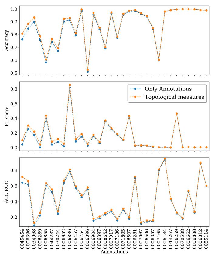
12Annotation prediction
Two models are trained for predicting gene annotations, one per
biological function (141 annotations). Namely, one in which the
topological measures of G are used and another one in which they
are not.
13Annotation prediction
14Annotation prediction
ID Biological process # Genes Max FP # FP
0006807 nitrogen compound metabolic process 15 41 1
0006289 nucleotide-excision repair 20 46 1
0006397 mRNA processing 17 48 1
0007017 microtubule-based process 18 49 1
0070588 calcium ion transmembrane transport 10 36 1
0006184 GTP catabolic process 49 47 1
0044267 cellular protein metabolic process 25 49 1
0007186 G-protein coupled receptor protein signaling ... 11 50 1
0006281 DNA repair 62 50 2
0006754 ATP biosynthetic process 24 49 3
0006904 vesicle docking involved in exocytosis 11 50 4
0055114 oxidation-reduction process 870 47 5
15Link prediction: Spectral Evolution of Twitter Mention Networks
Objective

   Evaluate various link prediction methods that underlie the spectral
   evolution model.
   Applies the spectral evolution model to networks of mentions
   between individuals who used trending political hashtags in Twitter
   between August 2017 and August 2018.

                                                                         16
Mention networks
The dataset consists of 31 mention networks between Twitter
users who defined their profile location as Colombia. These
networks capture conversations around a set of hashtags related to
popular political topics between August 2017 and August 2018.
17Mention networks
Users are represented by the set of vertices V and the set of edges
is denoted by E. There exists an edge {i, j} ∈ V × V between
users i and j, if user i uses a political hashtag (e.g.,
#eleccionesseguras) and mentions user j (via @username).
A mention network G = (V, E) is represented as a weighted
multi-graph without self-loops. Our analysis is based on the largest
connected component of the multi-graph, denoted by
Gc = (Vc , Ec ).
18Mention networks
Hashtag |Vc | |Ec |
0 abortolegalya 1282 1538
1 alianzasporlaseguridad 150 351
2 asiconstruimospaz 2405 6950
3 colombialibredefracking 1476 3127
4 colombialibredeminas 655 1421
5 dialogosmetropolitanos 932 4134
6 edutransforma 161 404
7 eleccionesseguras 2634 7969
8 elquedigauribe 2052 5272
9 frutosdelapaz 1479 3468
19Spectral evolution model
Let A denote the adjacency matrix of Gc . Furthermore, let
A = UΛUT denote the eigen decomposition of A, where Λ
represents the spectrum of Gc .
The spectral evolution model characterizes the dynamics of Gc
(i.e., how new edges are created over time) in terms of the
evolution of the spectrum of the network, assuming that its
eigenvectors in U remain unchanged.
20Spectral evolution model
If this condition is satisfied, estimating the formation of new
edges can be expressed as transformations of the spectrum
through the application of real functions (using graph kernels) or
extrapolation methods (using learning algorithms that estimate the
spectrum trajectories).
21Spectral evolution model verification
To apply the spectral evolution model, we need to verify the
assumption on the evolution of the spectrum and eigenvectors.
Every network Gc has a timestamp associated to each edge,
representing the time at which the edge is created.
• spectral evolution (eigenvalues),
• eigenvector evolution,
• eigenvector stability, and
• spectral diagonality test
22Spectral evolution model verification
300 1.0
0.8
200
Eigenvalues
0.6
u (T) ⋅ ui(t)|
100
0.4
| i
0
0.2
−100
0.0
0 10 20 30 40 0 250 500 750 1000 1250
Time period (Edge count) E(T)| - |E(t)| (Edge count)
|
(a) Spectral evolution (eigenvalues) (b) Eigenvector evolution
23Spectral evolution model verification
0 0
20 20 40
0.8
40
40
20
0.6
60
60
k (T)
80 0
0.4 80
100
100 −20
120 0.2
120
140 −40
0 50 100 140
( t)
k 0 50 100
(c) Eigenvector stability (eigenvalues) (d) Spectral diagonality test
24Growth models
Let K(A) be a kernel of an adjacency matrix A, whose eigen
decomposition is A = UΛUT . Graph kernels assume that there
exists a real function f (λ) that describes the growth of the
spectrum.
In particular, K(A) can be written as K(A) = UF (Λ)UT , for
some functions F (Λ) that applies a real function f (λ) to the
eigenvalues of A.
25Graph kernels
In particular, we use graph kernels of the triangle closing,
exponential and Neumann growth.
Kernel K(A) f (λ)
Triangle closing A2 f (λ) = λ2
Exponential exp(αA) f (λ) = eαλ
Neumann (I − αA)−1 1
f (λ) = 1−αλ
26Spectral Extrapolation
When the evolution of the spectrum is irregular it is not possible to
find a simple function that describe network growth. This model
extrapolates each eigenvalue of the network, assuming that the
network to be analyzed follows the spectral evolution model
27Performance
R2 RMSE
0.2
0.4
0.6
0.8
0.0
0.2
0.4
0.6
abortolegalya
alianzasporlaseguridad
asiconstruimospaz
colombialibredefracking
colombialibredeminas
dialogosmetropolitanos
edutransforma
eleccionesseguras
elquedigauribe
frutosdelapaz
garantiasparatodos
generosinideologia
hidroituangoescolombia
horajudicialur
lafauriecontralor
lanochesantrich
lapazavanza
Hashtags
tri
ext
exp
neu
libertadreligiosa
manifestacionpacifica
plandemocracia2018
plenariacm
proyectoituango
reformapolitica
rendiciondecuentas
rendiciondecuentas2017
resocializaciondigna
salariominimo
semanaporlapaz
serlidersocialnoesdelito
vocesdelareconciliacion
votacionesseguras
28Structural similarity
Structural similarity (SSIM) is a method for measuring similarity
between two images based on the idea that the pixels have strong
inter-dependencies especially when they are spatially close.
Adjacency matrices A and Âc are assumed to be images, and the
edges Aij and Âc,ij represent pixels.
29Performance
SSIM RMSE
0.7
0.8
0.9
0.0
0.2
0.4
0.6
abortolegalya
alianzasporlaseguridad
asiconstruimospaz
colombialibredefracking
colombialibredeminas
dialogosmetropolitanos
edutransforma
eleccionesseguras
elquedigauribe
frutosdelapaz
garantiasparatodos
generosinideologia
hidroituangoescolombia
horajudicialur
lafauriecontralor
lanochesantrich
lapazavanza
Hashtags
tri
ext
exp
neu
libertadreligiosa
manifestacionpacifica
plandemocracia2018
plenariacm
proyectoituango
reformapolitica
rendiciondecuentas
rendiciondecuentas2017
resocializaciondigna
salariominimo
semanaporlapaz
serlidersocialnoesdelito
vocesdelareconciliacion
votacionesseguras
30Conclusions
The extrapolation method tends to outperform the other methods
based on the performance metrics. Specifically, for 28 out of 31
networks (91% of the total), the extrapolation method provides
distinct, if slight, improvement.
The outperformance of the spectral extrapolation method seems to
be explained by the method being able to consider the irregular
evolution of the eigenvalues.
31Questions?
31Thanks!
31You can also read