NOx emission estimates during the 2014 Youth Olympic Games in Nanjing
←
→
Page content transcription
If your browser does not render page correctly, please read the page content below
Atmos. Chem. Phys., 15, 9399–9412, 2015
www.atmos-chem-phys.net/15/9399/2015/
doi:10.5194/acp-15-9399-2015
© Author(s) 2015. CC Attribution 3.0 License.

NOx emission estimates during the 2014 Youth Olympic Games
in Nanjing
J. Ding1,2 , R. J. van der A1 , B. Mijling1 , P. F. Levelt1,2 , and N. Hao3
1 RoyalNetherlands Meteorological Institute (KNMI), De Bilt, the Netherlands
2 Delft
      University of Technology, Delft, the Netherlands
3 German Aerospace Center (DLR), Oberpfaffenhofen, Germany

Correspondence to: J. Ding (jieying.ding@knmi.nl)

Received: 12 February 2015 – Published in Atmos. Chem. Phys. Discuss.: 4 March 2015
Revised: 31 July 2015 – Accepted: 12 August 2015 – Published: 24 August 2015

Abstract. The Nanjing Government applied temporary en-              a strong increase in NO2 concentrations without an increase
vironmental regulations to guarantee good air quality dur-          in NOx emissions. Furthermore, DECSO gives us important
ing the Youth Olympic Games (YOG) in 2014. We study                 information on the non-trivial seasonal relation between NOx
the effect of those regulations by applying the emission es-        emissions and NO2 concentrations on a local scale.
timate algorithm DECSO (Daily Emission estimates Con-
strained by Satellite Observations) to measurements of the
Ozone Monitoring Instrument (OMI). We improved DECSO
by updating the chemical transport model CHIMERE from               1   Introduction
v2006 to v2013 and by adding an Observation minus Fore-
cast (OmF) criterion to filter outlying satellite retrievals due    Reducing air pollution is one of the biggest environmen-
to high aerosol concentrations. The comparison of model re-         tal challenges currently in China. Nearly 75 % of urban ar-
sults with both ground and satellite observations indicates         eas are regularly polluted in a way that was considered un-
that CHIMERE v2013 is better performing than CHIMERE                suitable for their inhabitants in 2004 (Shao et al., 2006).
v2006. After filtering the satellite observations with high         In mega cities and their immediate vicinities, air pollutants
aerosol loads that were leading to large OmF values, unre-          exceed the Chinese Grade-II standard (80 µg m−3 for daily
alistic jumps in the emission estimates are removed. Despite        NO2 ) on 10–30 % of the days between 1999 to 2005 (Chan
the cloudy conditions during the YOG we could still see a de-       and Yao, 2008). Air pollution is directly related to the eco-
crease of tropospheric NO2 column concentrations of about           nomic growth in China and its accompanying increase of en-
32 % in the OMI observations when compared to the aver-             ergy consumption. In the last 2 decades, air pollutants per-
age NO2 columns from 2005 to 2012. The results of the im-           sistently increased in China. For instance, satellite measure-
proved DECSO algorithm for NOx emissions show a reduc-              ments showed that NO2 column concentrations increased by
tion of at least 25 % during the YOG period and afterwards.         about 50 % from 1996 to 2005 (Irie, 2005; Richter et al.,
This indicates that air quality regulations taken by the local      2005; van der A et al., 2006). By combining satellite obser-
government have an effect in reducing NOx emissions. The            vations with air quality models, Itahashi et al. (2014) showed
algorithm is also able to detect an emission reduction of 10 %      that the strong increase of NO2 columns over East China was
during the Chinese Spring Festival. This study demonstrates         caused by a doubling of NOx (NOx = NO + NO2 ) emissions
the capacity of the DECSO algorithm to capture the change           from 2000 to 2010. Zhang et al. (2007) found that NOx emis-
of NOx emissions on a monthly scale. We also show that the          sions increased by 70 % between 1995 and 2006 and Lam-
observed NO2 columns and the derived emissions show dif-            sal et al. (2011) found that anthropogenic NOx emissions in-
ferent patterns that provide complimentary information. For         creased 18.8 % during the period 2006 to 2009.
example, the Nanjing smog episode in December 2013 led to              Nanjing, the capital of Jiangsu Province, is a highly ur-
                                                                    banized and industrialized city located in East China, in

Published by Copernicus Publications on behalf of the European Geosciences Union.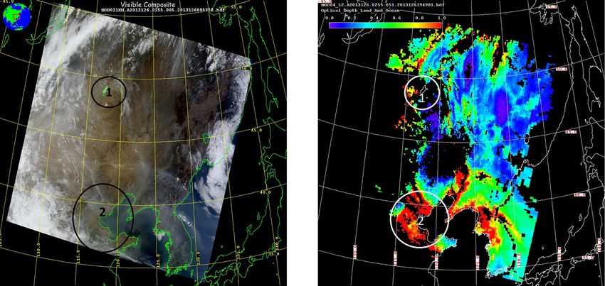
9400                                             J. Ding et al.: NOx emission estimates during the 2014 Youth Olympic Games

Table 1. Air-quality regulations taken by the Nanjing authorities in the year of YOG2014. The period is the start time of different regulations.
The italic regulations are still effective after the YOG.

                     Period             Regulations
                     1 May–30 June      The local government started to shut down the coal-burning factories.
                     1–15 July          All coal-burning factories have been shut down.
                     16–31 July         The work on one third of construction sites was stopped. The parking fees in
                                        downtown increased sevenfold.
                     1–15 August        The work on 2000 construction sites was stopped. Heavy-industry factories re-
                                        duced manufacturing by 20 percent. Vehicles with high emissions were banned
                                        from the city. Open space barbecue restaurants were closed. 900 electric buses
                                        and 500 taxis have been put into operation.
                     16–31 August       The work at all construction sites was put on hold.

the northwest part of the Yangtze River Delta (YRD). By                   emission reduction of 43.5 % based on mobile DOAS mea-
2012, the area of Nanjing had a population of 8.2 million                 surements. The emission reduction of NOx based on model
(Nanjing statistical Bureau, 2013). The YRD is one of the                 simulations was estimated to be about 40 % (Liu et al., 2013).
largest economic and most polluted regions in China. Tu et                   However, to study the effectiveness of the air quality mea-
al. (2007) found that the largest fraction of air pollution by            sures, it is not enough to look at the concentration measure-
NOx and SO2 can be attributed to local sources in Nanjing.                ments alone, as the reduction of air pollutants can also be
Li et al. (2011) concluded that air pollutant concentrations              affected by favorable meteorological conditions. Emissions
and visibility demanded urgent air pollution regulations in               need to be derived to better show the effect of temporary
the YRD region. From 16 to 29 August 2014, the Youth                      air quality regulations carried out for the Games. Up-to-date
Olympic Games (YOG) were held in Nanjing. To guaran-                      emission data are difficult to obtain, as most emission in-
tee good air quality during the Games, the city government                ventories are developed by a bottom-up approach based on
carried out temporary strict environmental regulations with               statistics on source sector, land-use and sector-specific emis-
35 directives from May to August. Other cities in the YRD                 sion factors.
cooperated with Nanjing to ensure good air quality during                    The bottom-up approach introduces large uncertainties
the Games. The periods with the main regulations are shown                in the emission inventories. To improve emission inven-
in Table 1. In addition, several technical improvements have              tories, a top-down approach can be used by estimating
been implemented to reduce pollution from heavy industry                  emissions from satellite observations (Streets et al., 2013).
and power plants.                                                         For constraining emissions of short-lived species, Martin et
   For previous major international events in China, local au-            al. (2003) used the ratio of the simulated to the observed
thorities have tried to comply with the air quality standards of          column to scale a priori emissions. They used optimal es-
the World Health Organization (WHO), which has a limit of                 timation to weigh the a priori emission inventory with the
200 µg m−3 for hourly NO2 concentrations. For each event,                 top-down estimates, resulting in an a posteriori inventory
the local government imposed restrictions on heavy indus-                 with error estimates. This method assumes that the relation-
try, construction and traffic. In 2008 the Beijing Munici-                ship between emissions and concentrations is not affected by
pal Government implemented a series of air pollution con-                 transport. Non-linear and non-local relations between emis-
trol measures for Beijing and surrounding cities to guarantee             sion and concentration can be indirectly solved by applying
good air quality for the 29th Olympic Games. These con-                   the method iteratively (e.g. Zhao and Wang, 2009), although
trol measures significantly reduced the emissions and con-                a posteriori error estimates are lost in this way. Kurokawa
centrations of pollutants. Satellite data show that the NO2               et al. (2009) and Stavrakou et al. (2008) used 4DVAR tech-
column concentrations decreased at least 40 % compared to                 niques to estimate emissions by applying an adjoint model of
previous years (Mijling et al., 2009; Witte et al., 2009). Both           the chemistry transport model to calculate the sensitivities.
bottom-up and top-down emission estimates show a decrease                 Another popular data assimilation method is the ensemble
of about 40 % in NOx emissions (Wang et al., 2009; Mi-                    Kalman filter (Evensen, 2003), which does not require an ad-
jling et al., 2013; Wang et al., 2010). During the 2010 World             joint model and is relatively easy to implement. As an exten-
Expo in Shanghai the NO2 column was reduced by 8 % from                   sion of the Kalman filter, it employs a Monte Carlo approach
May to August according to an analysis of Hao et al. (2011)               to represent the uncertainty of the model system with a large
of space-based measurements compared to previous years.                   stochastic ensemble. Whenever the filter requires statistics
In November 2010 emission reduction measures introduced                   such as mean and covariance, these are obtained from the
by the Guangzhou authorities also successfully improved air               sample statistics of the ensemble (Miyazaki et al., 2012).
quality for the Asian Games. Wu et al. (2013) claimed a NOx

Atmos. Chem. Phys., 15, 9399–9412, 2015                                                      www.atmos-chem-phys.net/15/9399/2015/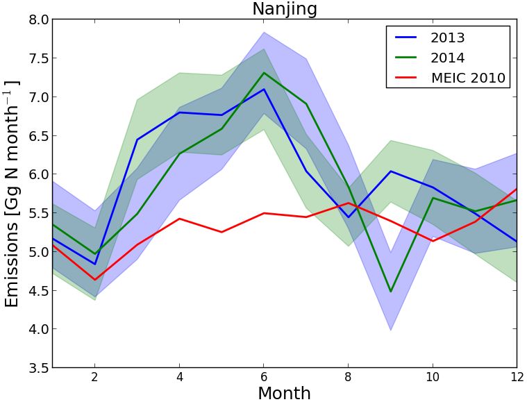
J. Ding et al.: NOx emission estimates during the 2014 Youth Olympic Games                                                    9401

   To get fast updates for short-lived air pollutants, Mi-           (ECMWF) with a horizontal resolution of approximately
jling and van der A (2012) designed a Daily Emission es-             25 × 25 km2 . The Multi-resolution Emission Inventory for
timates Constrained by Satellite Observation (DECSO) algo-           China (MEIC) (He, 2012) for 2010 gridded to a resolution
rithm. DECSO is an inversion method based on an extended             of 0.25◦ × 0.25◦ , is used for the initial emissions in DECSO.
Kalman filter. The algorithm only needs one forward model            Outside China, where no MEIC emissions are defined, the
run of a chemical transport model (CTM) to calculate all lo-         emission inventory of INTEX-B (Q. Zhang et al., 2009) is
cal and non-local emission/concentration relations. It updates       used. As the emission sector definition used in MEIC and
emissions by addition instead of scaling, enabling the detec-        INTEX-B does not match the 11 activity sectors according
tion of unaccounted emission sources.                                to the SNAP (Selected Nomenclature for Air Pollution) 97,
   In this study, we use the latest version of DECSO with            which are internally used in the CHIMERE model, we esti-
OMI satellite data to study how the environmental reg-               mate the redistribution of the emissions over the sectors (see
ulations affect the NOx emissions in Nanjing during the              Table 2).
2014 YOG. Detecting emission changes for Nanjing is chal-               As mentioned by Mijling and van der A (2012), to com-
lenging, as it is a smaller city than, e.g., Beijing. In addition,   pare CHIMERE simulations with satellite observations, we
Nanjing is in one of the most populated areas of China close         extend the modeled vertical profiles from 500 hPa to the
to Shanghai with a population of about 24 million. There-            tropopause by adding a climatological partial column, which
fore we have introduced a few improvements in the DECSO              is from an average of a 2003–2008 run of the global chem-
algorithm to better resolve small-scale emission changes in          istry transport model TM5. The simulated NO2 column con-
time and location. The improvements consist of an updated            centrations on the model grid are redistributed to the satel-
CTM and better filtering of erroneous satellite observations.        lite footprints. To enable direct comparison between simu-
The emission estimates will be based on the satellite observa-       lated and observed tropospheric vertical column, the averag-
tions of OMI, taking advantage of its high spatial resolution        ing kernel from the satellite retrieval is then applied to the
needed to resolve the changes in the Nanjing area. With this         modeled vertical profile.
improved algorithm we will compare the NOx emissions dur-               In this study, we used an updated version of DECSO,
ing the YOG with NOx emissions of the previous year in the           which is referred to as DECSO v3a. In particular, the cal-
Yangtze Delta River.                                                 culation speed has been improved in this update. DECSO
                                                                     does not distinguish between biogenic emissions and the an-
                                                                     thropogenic sectorial emissions. Emission differences are at-
2     Methods                                                        tributed to anthropogenic contribution only, i.e., the biogenic
                                                                     emissions are assumed to be modeled correctly by the CTM.
2.1    Emission estimates                                            Emission updates are distributed by ratio over the sectors
                                                                     (power, industry, transport, domestic) as described by the a
For the emission estimates of NOx over China we use the              priori emission inventory. If a grid cell is dominated by power
DECSO algorithm (Mijling and van der A, 2012). It uses               plant emissions, however, emission updates are attributed to
a CTM to simulate the NO2 concentrations and daily satel-            the power sector only. The locations of power plants are pro-
lite observations of NO2 column concentrations to constrain          vided to the algorithm as additional a priori information. In
NOx emissions. The algorithm is based on an extended                 DECSO v3a, the emission injection height has been made
Kalman filter to get new emission estimates by optimizing            sector-dependent. Emissions are injected in the lowest three
NO2 column concentrations of model and satellite observa-            model layers of the CTM; each sector having its own charac-
tions. The inclusion of sensitivities of NO2 column concen-          teristic vertical emission distribution. For example, transport
trations on the NOx emissions in other locations is an essen-        emissions are released at the surface, while power plant emis-
tial part of DECSO. A terrain-following trajectory analysis is       sions are fully released in the third model layer correspond-
used in this calculation to describe the transport of NO2 over       ing to a typical smokestack height. Trajectory calculations of
the model domain for a time interval between two overpasses          the observed species are crucial in the determination of the
of the satellite instrument. This approach results in a fast al-     source-receptor relations. The DECSO algorithm uses mete-
gorithm suitable for daily estimates of NOx emissions on a           orological wind fields (the same as used in the CTM) to cal-
0.25◦ × 0.25◦ resolution. A detailed description of DECSO            culate how the content of a tropospheric column is advected
v1 can be found in Mijling and van der A (2012).                     over the model domain. Here, the injection heights is dis-
   The CTM used in DECSO is CHIMERE (Schmidt, 2001;                  tributed according to the modeled vertical NOx distribution.
Bessagnet et al., 2004; Menut et al., 2013). CHIMERE is              In DECSO, the forward trajectory calculation is changed to a
implemented on a 0.25◦ × 0.25◦ spatial grid over East Asia           backward trajectory calculation, i.e., the source-receptor re-
from 18 to 50◦ N and 102 to 132◦ E. It contains eight at-            lations are calculated backward in time, based on the height
mospheric layers up to 500 hPa. The meteorological input             distribution of NOx modeled at satellite overpass time.
for CHIMERE is the operational meteorological forecast of               In DECSO v3a, tuned synthetic error estimates Eobs esti-
the European Centre for Medium-Range Weather Forecasts               mates are used, derived from the original satellite observation

www.atmos-chem-phys.net/15/9399/2015/                                                 Atmos. Chem. Phys., 15, 9399–9412, 2015
9402 J. Ding et al.: NOx emission estimates during the 2014 Youth Olympic Games
Table 2. Estimated redistribution of MEIC sectors over SNAP 97 sectors.
MEIC sectors SNAP 97 sectors Power Industry Transport Residential Agriculture
Combustion in energy and transformation industries 1 – – – –
Non-industrial combustion plants – – – 1 –
Combustion in manufacturing industry – 0.3 – – –
Production process – 0.3 – – –
Extraction and distribution of fossil fuels and geothermal energy – 0.4 – – –
Solvent and other product use – – – – –
Road transport – – 1 – –
Other mobile sources and machinery – – – – –
Waste treatment and disposal – – – – –
Agriculture – – – – 1
Other source and sinks – – – – –
via to a vertical column with the tropospheric air mass fac-
tor (AMF) (Boersma et al., 2007, 2011). DOMINO v2.0
Eobs = f · Esat + (1 − f ) · (0.5 · Esat ) , (1) mainly improves the NO2 air mass factor by improved ra-
csat
with f = e(− 2 ) , diative transfer, surface albedo, terrain height, clouds and
a priori vertical NO2 profiles. The bias between DOMINO
where Esat is the original observation error from the retrieval v2.0 and Multi-Axis Differential Optical Absorption Spec-
method and Csat is the retrieved NO2 column of the satellite troscopy (MAX-DOAS) ground observations at five loca-
observation. The unit in this formula is 1015 molecules cm−2 . tions is only −10 ± 14 % over China and Japan (Irie et al.,
The modified errors give more weight to satellite obser- 2012). The DOMINO algorithm does not explicitly account
vations with high values during the assimilation by re- for the effect of aerosols on the solar radiation. Rather it
ducing their relative error while maintaining the dominat- is indirectly accounted for by the higher cloud fraction in
ing absolute error for low values (typically around 0.5 × aerosol contaminated scenes. However, Lin et al. (2014) con-
1015 molecules cm−2 ). In this way, DECSO better captures cluded that especially in China the effects of aerosols and sur-
new emission points or high-emission episodes. face reflectance anisotropy have implications for retrievals of
NO2 from OMI and suggested that exclusion of high aerosol
2.2 Satellite observations
scenes supports better emission estimates at fine spatial and
In this study, satellite observations from the Dutch-Finnish temporal scales.
Ozone Monitoring Instrument (OMI) on NASA’s Aura satel- Since 25 June 2007, OMI data have been affected by the
lite (Levelt et al., 2006) are used in DECSO. The satellite so-called row anomaly, which deteriorates the spectral obser-
was launched on 15 July 2004 into a sun-synchronous polar vations for particular viewing directions of OMI (Boersma
orbit at 705 km altitude. OMI is a nadir-viewing spectrome- et al., 2011; Kroon et al., 2011). Twenty-nine out of the 60
ter measuring the atmosphere-backscattered solar light in the rows are affected by the row anomalies and no longer used
ultraviolet-visible (UV/VIS) range from 270 to 500 nm with after 1 January 2011. We also filter out the four pixels at ei-
a spectral resolution of about 0.5 nm. The 114◦ wide view ther side of the swath because the size of these pixels is 3
of OMI results in a swath width of 2600 km, providing daily times larger than the model grid cell. After the filtering, the
global coverage in about 14 orbits. The local overpass time largest footprint is about 75 × 21 km2 . To reduce the influ-
is around 13:30 local time (LT). The pixel size of OMI is ence of cloudy and bright surface scenes on the quality of the
24 × 13 km2 at nadir and increases to about 150 × 28 km2 at retrieval product, we use only observations having a surface
the end of the swath. albedo lower than 20 % to remove observations over snow
We use the tropospheric NO2 vertical column con- and ice (Product Specification Document of DOMINO v2 on
centrations retrieved with the Dutch OMI NO2 retrieval www.temis.nl). The observations with clouds below 800 hPa
(DOMINO) algorithm version 2 (Boersma et al., 2011). The are also filtered out as these retrievals are very sensitive to
data set is available on the Tropospheric Emissions Monitor- small differences in the NO2 profile shape and the retrieved
ing Internet Service (TEMIS) portal (http://www.temis.nl). cloud height. Mijling and van der A (2012) filter out the ob-
The DOMINO algorithm first obtains NO2 slant columns servations with a cloud fraction higher than 20 %. Based on
from the OMI reflectance spectra by using Differential Op- this filtering, there are no tropospheric NO2 satellite obser-
tical Absorption Spectroscopy (DOAS). After separating vations over Nanjing during the YOG due to the cloudy con-
the stratospheric and tropospheric contribution to the slant ditions at the overpass time of the satellite. Thus, to obtain
column, DOMINO converts the tropospheric slant column more NO2 satellite observations, we use observations with a
Atmos. Chem. Phys., 15, 9399–9412, 2015 www.atmos-chem-phys.net/15/9399/2015/J. Ding et al.: NOx emission estimates during the 2014 Youth Olympic Games 9403 Figure 1. Land use over the Jiangsu Province from Global Land Cover Facility (1994) (left) and the GlobCover Land Cover (2009) (right) and as used in CHIMERE v2006 and CHIMERE v2013. The eight categories are: 1. Urban, 2. Barren land, 3. Grassland, 4. Agricultural land, 5. Shrubs, 6. Needleleaf forest, 7. Broadleaf forest, 8. Water. The solid rectangle (about 50 × 90 km2 ) indicates the 6 grid cells that cover the Nanjing area. cloud radiance fraction lower than 70 % (comparable with a cloud fraction of about 30–35 %) instead of the cloud frac- tion lower than 20 %. From our analysis of the satellite data we conclude that as a result of this new limit on the cloud fraction the error on the measurements increases by less than 20 % and without introducing biases. Yet this effect is com- pensated by the advantage that more data become available. The number of observations over the whole domain increases by about 37 % on average. 2.3 Ground-based observations To validate the model results in Nanjing, we use avail- able independent measurements from the national in situ Figure 2. The diurnal cycle in Nanjing from January to August 2014 observation network, which are collected and maintained according to in situ observations, OMI-assimilated CHIMERE by the China National Environmental Monitoring Center v2013 and CHIMERE v2006. (CNEMC). The aqicn.org team publishes the hourly Air Quality Index (AQI) of specific air pollutants, such as NO2 , SO2 , and particulate matter (PM10 and PM2.5 ), on 3 Improvements of DECSO their website based on the measurements from CNEMC. The AQI is calculated by the conversion table from the 3.1 Model improvement Technical Regulation on Ambient Air Quality Index in China published by the Ministry of Environmental Pro- The performance of the CTM is important for the DECSO re- tection (http://kjs.mep.gov.cn/hjbhbz/bzwb/dqhjbh/jcgfffbz/ sults. CHIMERE v2006 is an outdated model version which 201203/W020120410332725219541.pdf). We use the same has been used in DECSO algorithm versions up to v3a. table to convert the AQI back to the surface concentration To improve the emission estimation results, we updated the unit of µg m−3 . For this study, the NO2 hourly in situ mea- CTM to CHIMERE v2013 (DECSO v3b). surements of Nanjing for the period of April 2013 to Decem- The new model adds biogenic emissions of six ber 2014 are used. The location of these measurements is the species: isoprene, α-ioporene, α-pinene, β-pinene, limonene, Nanjing People’s Government building, which is located in ocimene and NO. These biogenic emissions are calculated the center of Nanjing. Interpretation of the validation results by the model preprocessor using the MEGAN model and is troubled by the absence of peripheral information of the land use data (Menut et al., 2013). The added biogenic emis- in situ measurements. For instance, the type of instrument is sions can affect the emissions estimated for rural areas as unknown and the exact location of the measurement such as biogenic NO emissions in rural areas cannot be neglected the height or the distance to a local traffic road is unclear. in summertime. Compared to the old version of CHIMERE, www.atmos-chem-phys.net/15/9399/2015/ Atmos. Chem. Phys., 15, 9399–9412, 2015
9404 J. Ding et al.: NOx emission estimates during the 2014 Youth Olympic Games
the new model version includes a more advanced scheme for
secondary organic aerosol chemistry. In addition, the chem-
ical reaction rates are updated and a new transport scheme
is used in the new CHIMERE model. The new CHIMERE
model includes the emission injection height profile for dif-
ferent emission sectors. For CHIMERE v2013 we use the
same input data except for the land use data. We use land
use data from the GlobCover Land Cover (GCLC version
2.3) database, which are updated for the year 2009, while the
land use database included in CHIMERE v2006 is the Global
Land Cover Facility (GLFC) giving the land use of 1994. As
China is a fast developing country, the land use may have
large differences in 15 years due to urbanization (see Fig. 1).
Thus, the updated land use database will positively affect the
model simulations over China.
To assess the effect of the new CTM, we run DECSO Figure 3. The comparison of the absolute OmF
v3a and DECSO v3b for the period January 2013 to Au- (1015 molecules cm−2 ) of CHIMERE v2006 and CHIMERE
gust 2014. Figure 2 shows the comparison of the average v2013 for the whole East Asian domain from June to August. The
diurnal cycle of surface NO2 concentrations from the two colorbar represents the frequency of satellite observations for that
specific value of OmF.
CHIMERE models with in situ observations in Nanjing aver-
aged for January to August 2014. We select the 0.25◦ × 0.25◦
model grid cell that contains the in situ measurement lo- DECSO the daily Observation minus Forecasts (OmF) val-
cation. According to GCLC database, 70 % of the grid cell ues have been stored. The OmF is a common measure for
is urban area. We see that the surface NO2 concentration the forecasting capabilities of the model in the data assim-
of CHIMERE v2013 during nighttime is closer to the ob- ilation. We compare the absolute OmF of both models for
servations than for CHIMERE v2006. Our earlier model the summer (June to August) of 2014 in Fig. 3. In the Fig-
evaluations of CHIMERE showed that the nocturnal surface ure a linear regression is fitted through the data points that
NO2 concentrations simulated by CHIMERE v2006 are usu- shows the absolute OmF of CHIMERE v2013 is lower than
ally too high in urban areas caused by unrealistically low that of CHIMERE v2006 indicating a better performance
boundary layer heights and too little vertical diffusion. In of CHIMERE v2013 in summertime. However, the abso-
CHIMERE v2013, the boundary layer heights over urban lute OmF of two models is similar in wintertime. Since bio-
areas are limited by a minimum boundary layer height. As genic emissions are negligible in wintertime, this may point
expected, v2013 improves the surface concentration sim- to an effect of the missing biogenic emissions in the older
ulation at nighttime, while differences during daytime are version of CHIMERE. Based on these comparisons we se-
rather small compared to the in situ observations. We cal- lected CHIMERE v2013 in DECSO v3b for NOx emission
culate the bias and root mean square error (RMSE) be- estimates in this study.
tween the model results and in situ observations. The bias of
CHIMERE v2013 is 3.7 µg m−3 , which is 10 µg m−3 smaller 3.2 Quality control of satellite data
than for CHIMERE v2006. The difference of RMSE be-
tween the two models is very small: the RMSE of CHIMERE Earlier studies showed that the DOMINO v2 retrievals do
v2013 is 28 µg m−3 and of CHIMERE v2006 is 31 µg m−3 . not account enough for the effect of high aerosol concen-
For the satellite overpass time, the bias improves from 4.4 to trations on NO2 columns (see Sect. 2.2) and at the same
1.8 µg m−3 while the RMSE remains the same. However, in time we know that high aerosol concentrations are a signif-
urban areas the local sources have transient influences on in icant problem in most megacities in China. When checking
situ observations. Blond et al. (2007) concluded that urban in the time series of NOx emissions over Nanjing for 2013 by
situ observations of NO2 cannot be used for the validation of DECSO v3b, we find some suspicious fluctuations at partic-
a CTM model with low spatial resolution because the repre- ular days. At these dates the derived NOx emissions drop to
sentativeness of the in situ measurement for the grid cell is zero in 1 day and then slowly increase again to the previous
very low. In spite of this, by using the 8-month average of emission levels in the following days. These unrealistic emis-
the diurnal cycle to reduce the transient influences on the in sion updates concurred with extreme OmF values (lower than
situ measurements, we see some improvements for averaged −5 × 10¹⁵ or higher than 10 × 1015 molecules cm−2 ) with
NO2 concentrations in CHIMERE v2013. relative small OmF variances, which are calculated as the
In order to get a more comprehensive validation of the quadratic sum of model and observation errors (Fig. 4). In
model results, we compare the two CHIMERE models with the time period of our study there are 20 days with these ex-
OMI satellite observations. During the data assimilation of treme OmF values, 6 are positive and 14 are negative. All
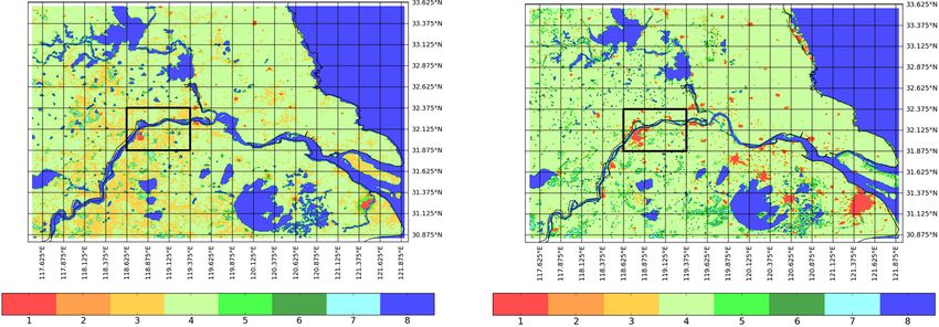
Atmos. Chem. Phys., 15, 9399–9412, 2015 www.atmos-chem-phys.net/15/9399/2015/J. Ding et al.: NOx emission estimates during the 2014 Youth Olympic Games 9405 Figure 4. The time series of the OmF from January 2013 to September 2014 for the single grid cell over the center of Nanjing. The error bar is the root mean square error of observations (Eobs ). are having a significant impact on the NOx emissions. For tection of outliers. A filter has to be implemented with care, most of those 20 days, the in situ observations of PM10 from to avoid the algorithm becoming insensitive to new emission CNEMC (see Sect. 2.3) show high aerosol concentrations, sources such as new power plants. Not losing sensitivity to which are above 100 µg m−3 in Nanjing. We also see a strong new emission sources is also the reason we do not choose a haze above Nanjing for all these 20 days from visual inspec- relative filter criterion. We select an OmF filter criterion in tion of the MODIS RGB images. In addition, we noticed that the range of [−5, 10] × 1015 molecules cm−2 based on our the MODIS images showed higher cloud fractions than the analysis discussed below. fractions retrieved from OMI observations. The deviating of The distribution of OmF of all pixels over our domain cloud fraction information from the OMI satellite retrieval is from January 2013 to September 2014 is Gaussian except probably due to the aerosol conditions, which are not taken for its tails and 97 % of the OmF is in the interval of into account in the cloud retrieval algorithm (Acarreta et al., [−5, 10] × 1015 molecules cm−2 . However, over highly pol- 2004; Stammes et al., 2008). High aerosol concentrations can luted areas both satellite observations and model results have not only complexly affect the cloud fraction and cloud pres- larger errors resulting in higher OmF values. In addition, sure retrieval but also directly affect the NO2 retrieval and the lifetime of NO2 is much longer in winter than in sum- results in either over- or under- estimated NO2 column con- mer. Therefore, the NO2 column concentration is higher than centrations (Lin et al., 2014). in summer, which may lead to large OmF values in win- Figure 5 shows an example of such an extreme case for ter time. We choose 15 high-polluted cities in China based East China on 6 May 2013 with high (positive) OmF values on AQI and study the distribution of the OmF for the sum- in combination with low observational uncertainties (Eq. 1). mer period (April to September 2013) and the winter pe- In the image we identify two areas with satellite observations riod (October 2013 to March 2014) (Fig. 7). As expected, that are at least 10 × 1015 molecules cm−2 higher than the the distribution of OmF is wider in winter than in summer. model forecast. One is over the Hulunbuir sand land at the In summer, 70 % of the OmF values are in the interval of border of China and Mongolia, the other one is around the [−5, 10] × 1015 molecules cm−2 , while in winter 50 % of the Bohai Bay. We compared the observations with the MODIS OmF values are within [−5, 10] × 1015 molecules cm−2 . We RGB and Aerosol Optical Depth (AOD) images on that day select an asymmetric interval because the assimilation is es- (Fig. 6). The MODIS AOD image shows high aerosol val- pecially sensitive to very negative outliers in OmF caused ues around the Bohai Bay and over the Hulunbuir sand land. by low observations (having small observational errors as- The RGB image of MODIS shows haze around the Bohai sociated), as opposed to very positive outliers caused by Bay, which indicates that high aerosol concentrations are pre- high observations, which are associated with large obser- sented in that area. However, the aerosol information is not vational errors. The observations with low error have more used in the retrieval of the DOMINO NO2 product leading to weight in the data assimilation process. To figure out the ef- NO2 observations that are strongly deviating from the model fect of a large OmF on NOx emission estimates, we com- forecast. pare a free run of CHIMERE v2013 with the MEIC in- The effect of high aerosol concentrations on the NO2 re- ventory with a run with the DECSO v3b assimilation. Dur- trieval is non-linear and depends strongly on both the type of ing the summertime, the difference in the seasonal average aerosol and its concentration. Also the height of the aerosol of the NO2 column concentration between these two runs layer and the presence of clouds play a role (Leitão et al., is 4.8 × 10¹⁵ molecules cm−2 in the Nanjing area (six grid 2010; Lin et al., 2014). It is therefore difficult to filter out out- cells). This column difference is caused by the NOx emission liers in the observed NO2 based on aerosol data. In the data difference of 9.2 × 10¹⁵ molecules cm−2 h−1 . From a sim- assimilation it is assumed that the OmF distribution is Gaus- ple back-of-the-envelope calculation we derive that a neg- sian and the OmF can be used to filter outliers from the data. ative 5 × 10¹⁵ molecules cm−2 difference in NO2 columns So far, no OmF outlier criterion has been used in DECSO. requires a 9.6 × 10¹⁵ molecules cm−2 h−1 emission change, Our previous analysis, however, shows the need for the de- which would mean that all NOx emissions in Nanjing would www.atmos-chem-phys.net/15/9399/2015/ Atmos. Chem. Phys., 15, 9399–9412, 2015
9406                                          J. Ding et al.: NOx emission estimates during the 2014 Youth Olympic Games

Figure 5. The comparison of the CHIMERE v2013 forecast (left) with OMI satellite observations (middle) on 6 May 2013. The right plot
shows the difference between observations and forecast (OmF).

                                                                    tions. For the in situ observations we select the monthly mean
                                                                    at 13:00 LT to be able to compare the results with the satel-
                                                                    lite observations whose overpass time is about 13:30 LT (see
                                                                    Fig. 8), which is also the average overpass time in Nanjing.
                                                                    Compared to the year 2013 the in situ measurements show no
                                                                    significant improvement in the surface NO2 concentration at
                                                                    13:00 LT for the period May to August 2014 when the gov-
                                                                    ernment took air quality regulations for the YOG. However,
                                                                    we see a high variability in the monthly averaged data, indi-
                                                                    cating that the data are strongly affected by highly variable
Figure 6. The RGB image (left) and Aerosol Optical Depth (right)    local sources (e.g. local traffic) and weather. We also calcu-
from MODIS on 6 May 2013. Circle 1 and circle 2 represent           late the monthly average using all measurements and we still
the Hulunbuir sand land and the Bohai Bay respectively. (The        see a high variability in the time series. Because of the high
figures are from https://ladsweb.nascom.nasa.gov/browse_images/     variability in the ground data and its low representativity for
granule_browser.html).                                              the whole city of Nanjing, we discarded this data set in our
                                                                    analysis.
                                                                       Figure 1 shows the land-use over Jiangsu Province. The
be removed in a single day. This change in emission is              rectangle referred to as the Nanjing area covers the whole
comparable to the total emissions of two large-sized coal-          of Nanjing including all industrial areas along the Yangtze
fired power plants. This shows that a change in OmF of              River. According to the MEIC sector distribution, the power
5 × 10¹⁵ molecules cm−2 is very unrealistic even in the most        plants in the selected area are dominating the NOx emissions.
extreme cases. Therefore, this limit will be used as a crite-       To study the effects of the air quality regulations for the YOG
rion to filter outliers, which are in general caused by wrong       on tropospheric NO2 column concentrations, we compare the
NO2 retrievals. To avoid the influence of the extreme OmF           monthly averages of satellite observations over the Nanjing
on emission estimates and still be able to monitor real emis-       area for each year from 2005 to 2014 by regridding the ob-
sion changes, we filter out negative OmF values lower than          servational data on the model grid over the area.
5×10¹⁵ molecules cm−2 and positive OmF values more than                The satellite observations show that on average the NO2
10 × 1015 molecules cm−2 to be conservative. After applying         column concentrations are rather similar from year to year
the OmF filter criteria, we filter out 16 % of the extreme OmF      (Fig. 9). Although a small increasing trend from 2005 to 2011
in the polluted cities and less than 3 % in the whole domain.       is visible in the satellite data, it is negligible compared to the
The large unrealistic jumps in emission disappear from the          SD of the natural variability. It is clear that the NO2 columns
time series.                                                        have a seasonal cycle that is lower in summer than in win-
                                                                    ter due to the seasonal change of the NO2 lifetime (van der
                                                                    A et al., 2006). Note that the small decrease in columns in
4   Emission analysis for the Nanjing Youth                         February might be caused by the reduced emissions during
    Olympic Games                                                   the Spring Festival (Q. Zhang et al., 2009). The monthly aver-
                                                                    ages of NO2 in situ observations shown by Wang et al. (2011)
First, we compare NO2 monthly average concentrations in             for Beijing, Shanghai and Guangzhou in 2005 were also re-
2014 with previous years using in situ and satellite observa-

Atmos. Chem. Phys., 15, 9399–9412, 2015                                               www.atmos-chem-phys.net/15/9399/2015/
J. Ding et al.: NOx emission estimates during the 2014 Youth Olympic Games 9407
Figure 7. The distribution of the OmF values over 15 polluted cities in summer (a) and in winter (b). The 15 polluted cities are Baoding,
Beijing, Chengdu, Harbin, Hohhot, Guangzhou, Jinan, Shanghai, Shenyang, Shijiazhuang, Tianjin, Wuhan, Xi’an, Xingtai and Zhengzhou.
smog period in Nanjing because stagnant air in the region
accumulated anthropogenic pollution. Compared to the av-
eraged NO2 column in August from 2005 to 2012, the NO2
column of August in 2014 is decreased by 32 % in Nanjing.
However, this significant decrease can be caused by the rainy
weather during that month. Thus, NOx emission estimates
are needed to show if the air quality regulations were really
effective. The emission estimates use not only satellite obser-
vations in the location of the YOG but use all observations
over China that are transported to and from Nanjing. Besides
transport of air, the meteorological effect on the lifetime of
NO2 is taken into account.
To compare the NOx emissions in Nanjing in 2014, es-
Figure 8. The monthly averaged in situ NO2 concentration at 13:00 pecially during the YOG, with the same period of the year
local time in Nanjing for 2013 and 2014. The bar is the standard 2013, we run DECSO v3b with the OmF criterion as de-
deviation (natural variability) of the observations for each month scribed in Sect. 3.2 from October 2012 to December 2014,
(derived from the daily data on www.aqicn.org). where the first 3 months are used as a spin-up period. Fig-
ure 10 shows the monthly NOx emissions in Nanjing for the
year 2013 and 2014 estimated by this version of DECSO.
For comparison the initial MEIC inventory is also plotted in
duced by around 10 % in February. We see that the NO2 col-
the figure. The NOx emissions have a different seasonal cy-
umn during the YOG period (August 2014) is on average
cle compared to the NO2 columns of satellite observations
only 6.6 × 10¹⁵ molecules cm−2 , which is the lowest value
in Nanjing. The months with high emissions are June and
among the last 10 years and more than 3 standard deviations
July while the highest NO2 columns of the satellite obser-
from the mean. Possibly due to the effect of the continuous
vations appear in January and December. According to the
air quality regulations for the YOG and afterwards, the NO2
sector distribution in the MEIC inventory, the emissions of
columns of the following months are also lower than for pre-
power plants and industrial activities are the main sources
vious years. The more permanent measures (traffic-related)
in Nanjing. At least 50 % of the total NOx emissions are
resulting from the YOG affect a small fraction of the total
from power plants and 40 % are from the industrial activi-
emissions. In November, the local government took similar
ties. H. Zhang et al. (2009) showed that the seasonal cycle of
air quality regulations for the first National Memorial cer-
the electricity consumption in Nanjing for the 7 years from
emony held on 13 December 2014. That might explain the
2000 to 2006 peaks in the summertime, because the electric-
lower NO2 columns of the last 2 months of 2014 compared to
ity consumption and power load are highly correlated with
those of 2013 and compared to the average of the last 8 years.
temperature in summer. The value of electricity consumption
However, it is still within the range of the standard deviation
in summer is at least two times higher than in winter every
of NO2 columns for the last 8 years. Differences from year
year and keeps increasing during those 7 years. The season-
to year can also be attributed to the meteorological condi-
ality of electricity consumption is caused by the increasing
tions (Lin et al., 2011). Particularly in December 2013, NO2
usage of air conditioning in the hot season, while there is no
columns are very high. This episode is well known as a heavy
www.atmos-chem-phys.net/15/9399/2015/ Atmos. Chem. Phys., 15, 9399–9412, 20159408 J. Ding et al.: NOx emission estimates during the 2014 Youth Olympic Games
Figure 10. The monthly NOx emission estimates by DECSO in
Nanjing for 2013 (blue line) and 2014 (green line) and the monthly
Figure 9. The monthly averages of OMI satellite observations of NOx emission of the MEIC inventory of 2010 (red line). The shade
tropospheric NO2 concentrations. The solid lines are the measure- areas show the error of the mean NOx emission estimates from
ments over the Nanjing area. The grey lines are the monthly aver- DECSO.
ages for each year from 2005 to 2012 to indicate the annual vari-
ability. The black lines show the average value for the years from
2005 to 2012. The bars are the standard deviations of monthly NO2 Figure 10 shows a large reduction of NOx emissions in
observations from 2005 to 2012.
September 2014. The total NOx emissions in September in
Nanjing are 4.5 Gg N. Compared to the same time of the year
heating system used in winter time in Nanjing. The oppo- 2013, the reduction is about 25 %. However, the emission re-
site cycles of column concentrations (Fig. 9) and emissions duction in this case seems to have a delay of 1 month. The
(Fig. 10) show that the high NO2 concentrations in winter shaded area in Fig. 10 represents the error on the derived
in Nanjing are mainly affected by the long lifetime of NOx , emissions without taking into account the error introduced
while the seasonal cycle of NOx emissions is reversed as a by the Kalman Filter time lag. Reductions in emissions at the
result of the increased electricity consumption in summer- end of August or the following months can appear with a time
time. The difference with the seasonal cycle of MEIC might lag in the Kalman filter results (see e.g Brunner et al., 2012).
be attributed to the fact that our results are derived on city- This time lag is not fixed but depends on the amount, interval,
level, while the seasonal cycle for bottom-up inventories are accuracy and distance of the observations and it is therefore
often derived on a national or provincial scale (e.g. Q. Zhang difficult to quantify. In our case, this is partly a consequence
et al., 2009). The monthly average temperatures from June to of the use of monthly means, while the regulations became
September are above 20◦ . The monthly temperatures in 2014 active at the end of August. It is also a consequence of the
did not deviate much from the climatological values. lack of satellite observations due to the rainy (and therefore
We see a drop in NOx emissions in February for both years cloudy) weather in the second half of August 2014 when the
calculated with DECSO, which is also visible in the MEIC YOG took place. For these kind of conditions, DECSO only
inventory of 2010 (Fig. 10). This jump is consistent with detects the full extent of the emission reduction in Septem-
the decrease of NO2 columns of the satellite observations ber. We also see a NOx emission reduction of 10 % in Au-
in February compared to the neighboring months. Compared gust 2013, compared to the neighboring months. One likely
to the neighboring months, the NOx emission reduction in reason for this reduction is that the Asian Youth Games were
February is about 10 % in 2013 and 2014. This NOx emis- held during that time. The local government also took mea-
sion decrease was also noticed by Q. Zhang et al. (2009) in sures to ensure good air quality for that event but they were
the INTEX-B inventory and likely to be caused by the re- not as strict as for the YOG in 2014. We conclude that the
duced industrial activities during the Spring Festival. Lin and NOx emission reduction detected by DECSO for the YOG
McElroy (2011) also showed that the Spring Festival causes period and afterwards was at least 25 %, showing that the air
a reduction of about 10 % on NOx due to the decrease of quality regulations taken by the local government were effec-
thermal power generation based on the analysis of several tive.
satellite observations. Interestingly, we do not see an increase
of NOx emissions in the December 2013 smog period. This
shows that the smog is caused by the meteorological condi- 5 Discussion and conclusions
tions rather than increased emissions.
In this study the effect of the air quality regulations of the lo-
cal government during the YOG in Nanjing in 2014 has been
Atmos. Chem. Phys., 15, 9399–9412, 2015 www.atmos-chem-phys.net/15/9399/2015/J. Ding et al.: NOx emission estimates during the 2014 Youth Olympic Games 9409
quantified by analyzing observations on the ground and from The quality of our emission estimates is highly related to
the satellite. The focus in this study was on the reduced NO2 the quality of the model and the satellite observations. We
concentrations and NOx emissions. We compared NO2 dur- improved the DECSO algorithm by using a new version of
ing the YOG period with previous years using the in situ and the CTM: CHIMERE v2013 instead of CHIMERE v2006.
the OMI satellite observations. The in situ observations have The comparison of OmF between two models showed that
a large variability, even after averaging on a monthly basis. CHIMERE v2013 has a better performance in summertime.
This is probably caused by the variability of local sources and Good quality of satellite observations is also essential for
it indicates that these in situ observations are not representa- emission estimates. The DOMINO retrieval algorithm does
tive for the larger area of Nanjing. The in situ data show no not properly account for the effects of high aerosol concen-
significant decrease during the YOG period. Since we have trations, which are common in China, on the retrieved NO2
no error estimates of the in situ observations and very little columns. In case of high aerosol concentrations, the differ-
information on the instrument and measurement techniques ence between the model simulations and the retrievals is very
we discard the results of the in situ observations in our con- large, which leads to wrong updates of NOx emissions in
clusions. DECSO. To improve the satellite observations we have set
For the view from space we limited ourselves to retrievals an OmF criterion to filter out erroneous observations and
of tropospheric NO2 from OMI, taking advantage of the high to avoid unrealistic NOx emission updates. We set the lim-
spatial resolution of OMI observations compared to similar itation to the range −5 to 10 × 1015 molecules cm−2 for the
instruments. The monthly OMI satellite observations showed OmF. With this filter criterion, the unrealistic updates of NOx
a 32 % decrease of the NO2 column concentration during emissions are mostly prevented. We will further analyze the
the YOG period in Nanjing compared to the average value impact of high aerosol concentrations on the retrieved NO2
for the last 10 years. However, the decrease of NO2 columns columns in future research.
observed by the satellite is not an objective measure to ver- Furthermore, we observed an opposite seasonal cycle of
ify the impact of the air quality regulations taken by the lo- NOx emissions compared to the NO2 columns observed by
cal government, because changes in NO2 columns can have OMI satellite. The seasonal cycle of NOx emissions is not
more causes such as horizontal transport of NO2 or increased the same for the whole China domain since the different cli-
wet deposition of the NO2 reservoir gas NO3 due to the rainy mate in the north and the south of China leads to a differ-
weather. Furthermore, due to cloudy conditions, the August ent seasonality of energy consumption during the year. In
average of 2014 is based on few observations. Therefore, it is Nanjing, as in most parts of southern China, people use air
important to analyze the emissions to show if the air quality conditioning in summer and do not use heating systems in
regulations have really affected the NO2 concentrations. winter. This leads to a larger electricity production of power
The results of our improved emission estimate algorithm plants in summer resulting in higher NOx emissions. Tu et
DECSO show that NOx emissions decreased by at least 25 % al. (2007) studied the air pollutants in Nanjing and also found
in September 2014, which shows that the air quality regula- high NO2 columns in winter but concluded that the high NO2
tions were effective during the YOG period and that only a columns were caused by high NOx emissions in winter, while
small part of the reduced NO2 column concentrations were our emission estimates show the opposite. Wang et al. (2007)
caused by the weather conditions. However, the reduction analyzed the seasonality of NOx emissions based on GOME
has a 1 month delay in our results. This is because satellite satellite observations for the regions north and south of the
observations were scarce in the Nanjing area during the YOG Yangtze River, defined as north and south China. Their re-
(16 to 29 August), causing the DECSO algorithm to converge sults of south China showed the same seasonal cycle of NO2
slower to the new emissions, which is typical for the Kalman columns but a very weak seasonality of NOx emissions and
filter approach used in DECSO. Although the strong point of they also concluded that the NOx lifetime mainly determines
Kalman Filter is its detailed error analysis, this time lag is the NO2 columns. Ran et al. (2009) explained high NOx
not incorporated in its error formalism. In future research we concentrations in winter are caused by slower chemical pro-
intend to reduce this time lag by using a smoothing Kalman cesses and shallow boundary layers contributing to accumu-
filter technique. lation of NOx . The table in Wang et al. (2012) of annual
We were able to see the emission reduction of NOx in the and summer NOx emissions from coal-fired power plants
selected six grid cells representative for the Nanjing area. in 2005–2007 for different provinces in China showed that
That means that DECSO is at least able to estimate NOx the NOx emissions in Jiangsu Province in summer are higher
emissions on a spatial resolution of about 50 × 90 km2 . If we than mean seasonal emissions.
apply the same analysis on single grid cells the results are In conclusion, we not only found a reversed seasonal cycle
noisier because the footprint of the OMI covers on average peaking in summertime in the emission estimates, but also
a larger area than a single grid cell. To achieve emission es- indications for reduced emissions during the Spring Festival,
timates in a smaller area, either satellite observations with a the Asian Youth Games in 2013 and the YOG 2014. Based
higher spatial resolution are required or longer time periods on our emission estimates the air quality regulation during
should be considered. the YOG 2014 and afterwards reduced the NOx emissions
www.atmos-chem-phys.net/15/9399/2015/ Atmos. Chem. Phys., 15, 9399–9412, 20159410 J. Ding et al.: NOx emission estimates during the 2014 Youth Olympic Games
by at least 25 percent. This, together with favorable meteo- Chan, C. and Yao, X.: Air pollution in mega cities in China, Atmos.
rological conditions, was responsible for a decrease of 32 % Environ., 42, 1–42, doi:10.1016/j.atmosenv.2007.09.003, 2008.
in NO2 column concentrations observed from space. For the Evensen, G.: The Ensemble Kalman Filter: theoretical formula-
case of the YOG, our results can help the local government tion and practical implementation, Ocean Dynam., 53, 343–367,
to identify the impact of their air quality regulations on re- doi:10.1007/s10236-003-0036-9, 2003.
Hao, N., Valks, P., Loyola, D., Cheng, Y. F., and Zimmer, W.: Space-
ducing NOx emissions.
based measurements of air quality during the World Expo 2010
in Shanghai, Environ. Res. Lett., 6, 044004, doi:10.1088/1748-
The Supplement related to this article is available online 9326/6/4/044004, 2011.
at doi:10.5194/acp-15-9399-2015-supplement. He, K.: Multi-resolution Emission Inventory for China (MEIC):
model framework and 1990–2010 anthropogenic emissions,
in: International Global Atmospheric Chemistry Conference,
17–21 September, Beijing, China, available at: http://adsabs.
harvard.edu/abs/2012AGUFM.A32B..05H (last access: 4 Febru-
Acknowledgements. The research was part of the GlobEmission ary 2015), 2012.
Project funded and supported by the European Space Agency. We Irie, H.: Evaluation of long-term tropospheric NO2 data obtained
acknowledge Tsinghua University for providing the MEIC inven- by GOME over East Asia in 1996–2002, Geophys. Res. Lett.,
tory and the ESA GlobCover 2009 Project for the land use data set. 32, L11810, doi:10.1029/2005GL022770, 2005.
The MODIS images used in this study were acquired as part of the Irie, H., Boersma, K. F., Kanaya, Y., Takashima, H., Pan, X., and
NASA’s Earth-Sun System Division and archived and distributed Wang, Z. F.: Quantitative bias estimates for tropospheric NO2
by the MODIS Adaptive Processing System (MODAPS). The OMI columns retrieved from SCIAMACHY, OMI, and GOME-2 us-
is part of the NASA Earth Observing System (EOS) Aura satellite ing a common standard for East Asia, Atmos. Meas. Tech., 5,
payload. The OMI project is managed by the Netherlands Space 2403–2411, doi:10.5194/amt-5-2403-2012, 2012.
Office (NSO) and the Royal Netherlands Meteorological Institute Itahashi, S., Uno, I., Irie, H., Kurokawa, J.-I., and Ohara, T.: Re-
(KNMI). gional modeling of tropospheric NO2 vertical column density
over East Asia during the period 2000–2010: comparison with
Edited by: G. Frost multisatellite observations, Atmos. Chem. Phys., 14, 3623–3635,
doi:10.5194/acp-14-3623-2014, 2014.
Kroon, M., de Haan, J. F., Veefkind, J. P., Froidevaux, L., Wang,
References R., Kivi, R., and Hakkarainen, J. J.: Validation of operational
ozone profiles from the Ozone Monitoring Instrument, J. Geo-
Acarreta, J. R., De Haan, J. F., and Stammes, P.: Cloud pressure phys. Res., 116, D18305, doi:10.1029/2010JD015100, 2011.
retrieval using the O2 -O2 absorption band at 477 nm, J. Geophys. Kurokawa, J., Yumimoto, K., Uno, I., and Ohara, T.: Adjoint inverse
Res., 109, D05204, doi:10.1029/2003JD003915, 2004. modeling of NOx emissions over eastern China using satellite
Bessagnet, B., Hodzic, A., Vautard, R., Beekmann, M., observations of NO2 vertical column densities, Atmos. Environ.,
Cheinet, S., Honoré, C., Liousse, C., and Rouil, L.: Aerosol 43, 1878–1887, doi:10.1016/j.atmosenv.2008.12.030, 2009.
modeling with CHIMERE – preliminary evaluation at Lamsal, L. N., Martin, R. V., Padmanabhan, A., van Donke-
the continental scale, Atmos. Environ., 38, 2803–2817, laar, A., Zhang, Q., Sioris, C. E., Chance, K., Kurosu,
doi:10.1016/j.atmosenv.2004.02.034, 2004. T. P., and Newchurch, M. J.: Application of satellite ob-
Blond, N., Boersma, K. F., Eskes, H. J., van der A, R. J., servations for timely updates to global anthropogenic NOx
Van Roozendael, M., De Smedt, I., Bergametti, G., and Vau- emission inventories, Geophys. Res. Lett., 38, L05810,
tard, R.: Intercomparison of SCIAMACHY nitrogen dioxide doi:10.1029/2010GL046476, 2011.
observations, in situ measurements and air quality modeling Leitão, J., Richter, A., Vrekoussis, M., Kokhanovsky, A., Zhang, Q.
results over Western Europe, J. Geophys. Res., 112, 1–20, J., Beekmann, M., and Burrows, J. P.: On the improvement of
doi:10.1029/2006JD007277, 2007. NO2 satellite retrievals – aerosol impact on the airmass factors,
Boersma, K. F., Eskes, H. J., Veefkind, J. P., Brinksma, E. J., van Atmos. Meas. Tech., 3, 475–493, doi:10.5194/amt-3-475-2010,
der A, R. J., Sneep, M., van den Oord, G. H. J., Levelt, P. F., 2010.
Stammes, P., Gleason, J. F., and Bucsela, E. J.: Near-real time Levelt, P. F., van den Oord, G. H. J., Dobber, M. R., Malkki, A.,
retrieval of tropospheric NO2 from OMI, Atmos. Chem. Phys., Stammes, P., Lundell, J. O. V., and Saari, H.: The ozone monitor-
7, 2103–2118, doi:10.5194/acp-7-2103-2007, 2007. ing instrument, IEEE T. Geosci. Remote Sens., 44, 1093–1101,
Boersma, K. F., Eskes, H. J., Dirksen, R. J., van der A, R. J., doi:10.1109/TGRS.2006.872333, 2006.
Veefkind, J. P., Stammes, P., Huijnen, V., Kleipool, Q. L., Sneep, Li, L., Chen, C. H., Fu, J. S., Huang, C., Streets, D. G., Huang,
M., Claas, J., Leitão, J., Richter, A., Zhou, Y., and Brunner, D.: H. Y., Zhang, G. F., Wang, Y. J., Jang, C. J., Wang, H. L.,
An improved tropospheric NO2 column retrieval algorithm for Chen, Y. R., and Fu, J. M.: Air quality and emissions in the
the Ozone Monitoring Instrument, Atmos. Meas. Tech., 4, 1905– Yangtze River Delta, China, Atmos. Chem. Phys., 11, 1621–
1928, doi:10.5194/amt-4-1905-2011, 2011. 1639, doi:10.5194/acp-11-1621-2011, 2011.
Brunner, D., Henne, S., Keller, C. A., Reimann, S., Vollmer, M. K., Lin, J.-T. and McElroy, M. B.: Detection from space of a reduction
O’Doherty, S., and Maione, M.: An extended Kalman-filter for in anthropogenic emissions of nitrogen oxides during the Chi-
regional scale inverse emission estimation, Atmos. Chem. Phys.,
12, 3455–3478, doi:10.5194/acp-12-3455-2012, 2012.
Atmos. Chem. Phys., 15, 9399–9412, 2015 www.atmos-chem-phys.net/15/9399/2015/You can also read