ECOGRAPHY Research Exploring timescales of predictability in species distributions
←
→
Page content transcription
If your browser does not render page correctly, please read the page content below
ECOGRAPHY
Research
Exploring timescales of predictability in species distributions

Stephanie Brodie, Briana Abrahms, Steven J. Bograd, Gemma Carroll, Elliott L. Hazen,
Barbara A. Muhling, Mercedes Pozo Buil, James A. Smith, Heather Welch and Michael G. Jacox

S. Brodie (https://orcid.org/0000-0003-0869-9939) ✉ (sbrodie@ucsc.edu), S. J. Bograd, E. L. Hazen, B. A. Muhling, M. Pozo Buil, J. A. Smith, H. Welch
and M. G. Jacox, Inst. of Marine Science, Univ. of California Santa Cruz, Santa Cruz, CA, USA. SBr, SBo, ELH, MPB, HW and MGJ also at:
Environmental Research Division, NOAA Southwest Fisheries Science Center, Monterey, CA, USA. BAM and JAS also at: Fisheries Research Division,
NOAA Southwest Fisheries Science Center, San Diego, CA, USA. – B. Abrahms, Center for Ecosystem Sentinels, Dept of Biology, Univ. of Washington,
Seattle, WA, USA. – G. Carroll, School of Aquatic and Fisheries Sciences, Univ. of Washington, Seattle, WA, USA, and: Resource Ecology and Ecosystem
Modelling Group, NOAA Alaska Fisheries Science Center, Seattle, WA, USA.

Ecography                                       Accurate forecasts of how animals respond to climate-driven environmental change
44: 1–13, 2021                                  are needed to prepare for future redistributions, however, it is unclear which temporal
doi: 10.1111/ecog.05504                         scales of environmental variability give rise to predictability of species distributions.
                                                We examined the temporal scales of environmental variability that best predicted
Subject Editor:                                 spatial abundance of a marine predator, swordfish Xiphias gladius, in the California
Christine N. Meynard                            Current. To understand which temporal scales of environmental variability provide
Editor-in-Chief: Miguel Araújo                  biological predictability, we decomposed physical variables into three components: a
Accepted 16 February 2021                       monthly climatology (long-term average), a low frequency component representing
                                                interannual variability, and a high frequency (sub-annual) component that captures
                                                ephemeral features. We then assessed each component’s contribution to predictive skill
                                                for spatially-explicit swordfish catch. The monthly climatology was the primary source
                                                of predictability in swordfish spatial catch, reflecting the spatial distribution associated
                                                with seasonal movements in this region. Importantly, we found that the low frequency
                                                component (capturing interannual variability) provided significant skill in predicting
                                                anomalous swordfish distribution and catch, which the monthly climatology cannot.
                                                The addition of the high frequency component added only minor improvement in
                                                predictability. By examining models’ ability to predict species distribution anomalies,
                                                we assess the models in a way that is consistent with the goal of distribution forecasts
                                                – to predict deviations of species distributions from their average historical locations.
                                                The critical importance of low frequency climate variability in describing anomalous
                                                swordfish distributions and catch matches the target timescales of physical climate
                                                forecasts, suggesting potential for skillful ecological forecasts of swordfish distribu-
                                                tions across short (seasonal) and long (climate) timescales. Understanding sources of
                                                prediction skill for species environmental responses gives confidence in our ability to
                                                accurately predict species distributions and abundance, and to know which responses
                                                are likely less predictable, under future climate change. This is important as climate
                                                change continues to cause an unprecedented redistribution of life on Earth.

                                                Keywords: climate change, ecological forecasting, prediction, spatial ecology, species
                                                distribution models, temporal decomposition

                                                ––––––––––––––––––––––––––––––––––––––––
                                                © 2021 The Authors. Ecography published by John Wiley & Sons Ltd on behalf of Nordic Society Oikos
www.ecography.org                               This is an open access article under the terms of the Creative Commons
                                                Attribution License, which permits use, distribution and reproduction in any
                                                medium, provided the original work is properly cited.                                            1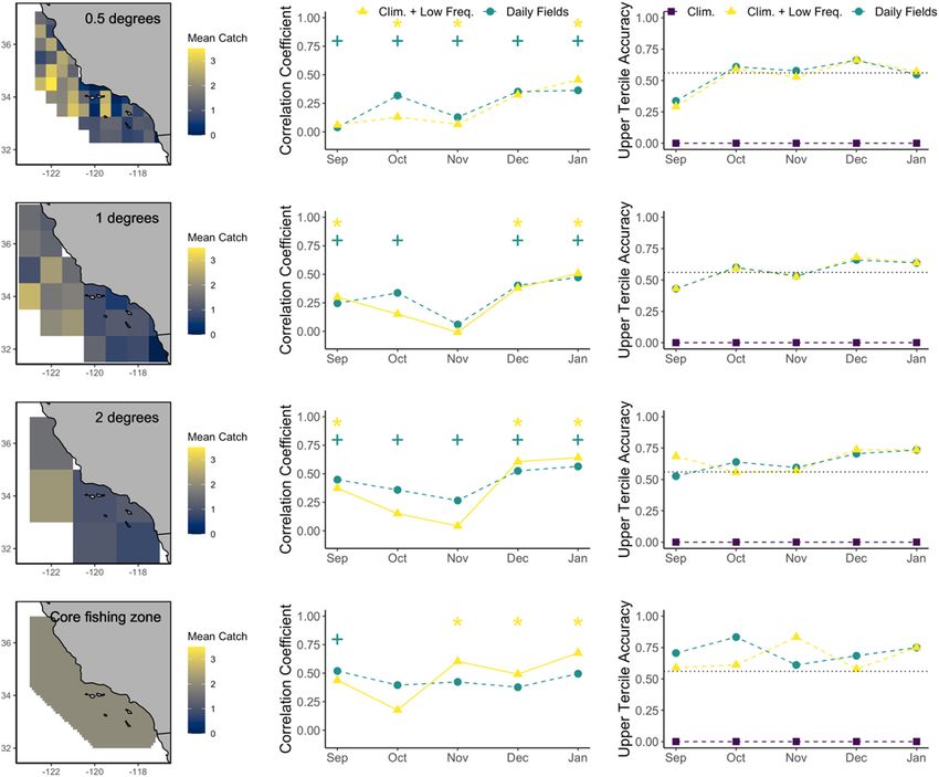
Introduction                                                           Ecological forecasting is gaining traction as an approach
                                                                   to understand, predict and project future ecosystem change
Our oceans are experiencing unprecedented climate-driven           (Tommasi et al. 2017, Dietze et al. 2018, Hobday et al. 2018,
changes. The magnitude and direction of these changes vary         Jacox et al. 2020). In marine systems, ecological forecasting
widely across space and time, causing species to respond in        most often relies on correlative statistical models applied to
diverse ways (Walther et al. 2002). For example, long-term         ocean climate forecasts (Payne et al. 2017). This makes skill-
changes in temperature and other physical properties have          ful ecological forecasts at a particular spatiotemporal scale
led to documented spatial (Perry et al. 2005, Tingley et al.       reliant on skillful forecasts of environmental variables at that
2009, Pinsky et al. 2013), behavioural (Mueller et al. 2011)       same spatiotemporal scale (Jacox et al. 2020). For example,
and phenological shifts (Edwards and Richardson 2004,              if a physical ocean forecast is unable to skillfully resolve
Kharouba et al. 2018, Szesciorka et al. 2020) across an            fine-scale ephemeral features such as eddies and fronts, an
increasingly diverse array of species. In addition, ephem-         ecological forecast reliant on physical variables cannot skill-
eral events such as heatwaves, storms and drought have             fully predict at these fine spatiotemporal scales. Similarly, if a
caused catastrophic population declines and restructuring          physical or ecological forecast derives its skill from long-term
of ecological communities (Boersma and Rebstock 2014,              climatological conditions, then forecasting is redundant and
Descamps et al. 2015, Smale et al. 2019). There remains            a monthly climatology can instead be used for short-term
considerable uncertainty and variability in the magni-             predictive purposes. Exploring which temporal scales of envi-
tude and direction of species’ responses to climate change         ronmental variability underpin our ability to predict species
and extreme climate events (Parmesan and Yohe 2003,                distributions is therefore essential to assess and improve the
Hazen et al. 2013, Pinsky et al. 2013, Poloczanska et al.          utility of ecological forecasting applications.
2013, Smale et al. 2019). Accurate predictions of these                Our goal is to understand the temporal scales of environ-
responses are paramount for informing proactive climate-           mental variability that provide predictability for spatially-
ready management.                                                  explicit animal abundance. We use data from a swordfish
    Species distributions can be considered a function of mul-     Xiphias gladius fishery in the California Current System
tiple scales of environmental variability (Winkler et al. 2014).   (CCS) to test the hypothesis that multiple scales of envi-
For example, many migratory taxa respond to environmen-            ronmental variability contribute to predictive skill of species
tal information over a range of timescales, including both         distributions. We use an approach that decomposes impor-
proximate conditions resulting from short-term environ-            tant environmental drivers into sub-annual, inter-annual and
mental variability (Boustany et al. 2010, Aikens et al. 2017,      climatological components, to quantify which scales pre-
Snyder et al. 2017) as well as long-term historical (i.e. cli-     dictably structure distributions and movements of animals.
matological) conditions (Abrahms et al. 2019a, Tsalyuk et al.      Importantly, we quantify model performance not just for
2019, Horton et al. 2020). Indeed, considering fine-scale          species distributions but also for species distribution anoma-
environmental variability (Hazen et al. 2018, Morán-               lies (i.e. deviations from climatological fisheries catch), which
Ordóñez et al. 2018, Abrahms et al. 2019b) or seasonal to          is key to assessing models’ capabilities to predicting future
inter-annual environmental variability (Zimmermann et al.          change in distributions. Our approach of modelling species
2009, Reside et al. 2010, Descamps et al. 2015, Thorson            distributions using abundance data is standard for fisheries
2019) can improve predictions of species spatial distribu-         datasets and for the species distribution modelling literature
tions in response to environmental change. There is a need         (Guisan and Thuiller 2005, Elith and Leathwick 2009). An
to better understand and define the relative contribution of       improved accounting of the temporal scales of environmental
different temporal scales of environmental variability to bet-     forcing that drive species distributional changes will aid in
ter predict species’ responses to future environmental change.     prioritizing monitoring and planning adaptive management
    Correlative species distribution models (SDMs) have            scenarios under climate variability and change.
become an important tool to predict and plan for changes
in species abundance and distribution under climate change
(Elith and Leathwick 2009, Robinson et al. 2017, Araújo et al.     Methods
2019, Brodie et al. 2020). While correlative models pro-
vide important insights into species’ realized niches under        Study system and focal species
observed conditions, there is a discrepancy among studies
as to whether species–environment correlations may break           The CCS is a highly productive and dynamic ecosystem in
down (Muhling et al. 2020), or hold up (Becker et al. 2019),       the northeast Pacific, dominated by seasonal upwelling that
under novel environmental conditions (Sequeira et al. 2018,        drives cool, nutrient-rich waters to the surface and stimu-
Yates et al. 2018). As climate change is driving non-stationar-    lates extensive biological productivity (Hickey 1979, Huyer
ity in ecosystems and reducing the utility of historical climate   1983). This ecosystem provides important foraging grounds
information (Zimmermann et al. 2009, Zurell et al. 2009,           for many highly migratory species, including species of
Franklin 2010), there is a need to understand which scales of      importance to fisheries (Block et al. 2011). Variability in the
environmental variability contribute to predictive skill (i.e.     CCS occurs across a range of spatial (meters to 1000s of km)
predictive ability) in SDMs.                                       and temporal scales, including intra-annual (e.g. upwelling,

2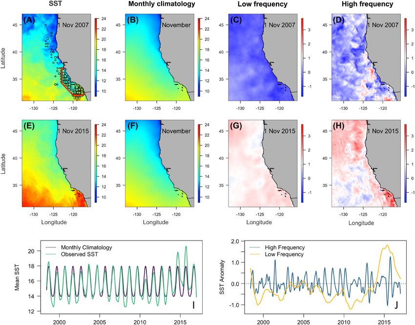
mesoscale features), interannual (e.g. due to large-scale cli-       Environmental data
mate modes like El Niño-Southern Oscillation) and multi-
decadal scales (e.g. due to decadal climate oscillations and         Environmental data (1998–2016) were sourced from a data-
secular climate change) (Checkley Jr and Barth 2009).                assimilative configuration of the Regional Ocean Modelling
These changes in the regional climate and oceanography               System (ROMS) that covers the CCS from 30 to 48°N and
can have pronounced ecological impacts; for example, a               from the coast to 134°W at 0.1° (~10 km) horizontal reso-
severe marine heatwave from 2014 to 2016, with positive              lution ( version
sea surface temperature anomalies up to 6°C (Bond et al.             2016a; Neveu et al. 2016; Fig. 1). Vertical structure in the
2015, Leising et al. 2015, Jacox et al. 2016), led to a broad        ROMS model is resolved by 42 terrain-following vertical
range of ecosystem impacts including species redistribut-            levels (Veneziani et al. 2009). Daily sea surface temperature
ing across the CCS (Cavole et al. 2016, Becker et al. 2018,          (SST; °C) and isothermal layer depth (ILD; m), defined as
Muhling et al. 2020).                                                the depth corresponding to a 0.5°C temperature difference
   Swordfish are a large highly migratory predator widely dis-       relative to the surface, were sourced from ROMS. Satellite-
tributed across the Pacific, Atlantic and Indian oceans (~50°N,      derived chlorophyll-a (Chl; mg m−3) was a 4 km 8-day com-
50°S). Swordfish exhibit extreme diel vertical migration, and        posite from GlobColour sourced from Copernicus Marine
in the CCS forage at depths up to 500 m during the day               Environment Monitoring Service and interpolated to the
and in surface waters at night (Sepulveda et al. 2010, 2018,         ROMS resolution (daily and 0.1° resolution). Environmental
Dewar et al. 2011). The CCS is an important foraging ground          covariates were selected based on published relationships of
for north Pacific swordfish, with some adults undertaking            swordfish distribution and catch in the CCS (Scales et al.
spawning migrations to tropical waters near Hawaii during            2017b, Brodie et al. 2018, Smith et al. 2020).
May–August (Grall et al. 1983) and other adults residing in              For each grid cell, three environmental covariates (SST,
the CCS year-round (Abecassis et al. 2012, Sepulveda et al.          ILD, Chl) were temporally decomposed into three compo-
2020). Within the CCS, swordfish are generally distributed           nent signals: 1) a monthly climatology; 2) a low-frequency
at higher latitudes in summer and lower latitudes in winter          component; 3) a high frequency component. The monthly
(Hanan et al. 1993, Sepulveda et al. 2018), with some indi-          climatology captures the mean historical seasonal cycle, with
viduals showing high site fidelity following extensive seasonal      conditions for each month averaged across all years (1998–
movements (Sepulveda et al. 2020). The presence and distri-          2016). Daily anomalies for each variable were calculated by
bution of swordfish in the CCS thus depend on a complex              subtracting the monthly climatology from the daily time
combination of movements across multiple scales, including           series at each grid point. The low frequency component was
large-scale spawning migrations, non-spawning seasonal lati-         calculated by smoothing the anomalies with a 12-month run-
tudinal movements, fine-scale foraging, diel vertical migra-         ning mean centered on each day in the time period (1998–
tion and site fidelity. As such, swordfish are an appropriate        2016). This low frequency component captures interannual
case study species to explore the sources of predictability in       variability in the oceanic environment. The high frequency
species distribution models.                                         component was the component remaining after subtracting
                                                                     the monthly climatology and low frequency components
Species data                                                         from the daily values. This high frequency component iso-
                                                                     lates sub-annual variability including ephemeral features such
Swordfish are available to U.S. fisheries in the CCS, and his-       as fronts and eddies. The monthly climatology, low-frequency
torically have largely been targeted with drift gillnet gear, in     and high-frequency components sum to the daily values of
contrast to longlines used in other large marine ecosystems          the observed environmental covariates.
(Hanan et al. 1993, Urbisci et al. 2016). The fishery operates           Our approach to decomposing environmental variables
primarily from September to January along the U.S. West              was designed with an eye toward assessing SDMs for fore-
Coast, deploying drift gillnet gear at night when swordfish          casting applications. In this sense, the monthly climatology
are shallower in the water column and susceptible to this            provides a baseline against which forecasts can be measured.
gear type. Gear will drift on average ~10 km during sets,            If the high and low frequency components do not apprecia-
so we consider the resolution of catch data to be approxi-           bly increase model performance relative to the monthly cli-
mately 0.1°. Swordfish catch data were obtained from the             matology, then a forecast is unnecessary. The low frequency
NOAA National Marine Fisheries Service observer program,             component isolates interannual variability (i.e. how a specific
which has placed observers on drift gillnet vessels since 1990       year differs from an ‘average’ year). Capturing interannual
(Caretta et al. 2004). Catch data were reported as the number        variability is the target of climate forecasts that are used as
of swordfish caught in each drift gillnet set, with multiple sets    the basis for SDM forecasts, so our analysis evaluates whether
per fishing trip, and set-level effort reported as duration (h) of   timescales of predictive skill in the climate forecasts align with
each set. Catch data for SDM training were temporally lim-           timescales of predictive skill in the SDM. Model performance
ited to 1998–2016 (n = 4162 sets, totaling 8788 swordfish            for interannual variability is also key to informing manage-
caught) to match the availability of satellite-derived chloro-       ment actions that are taken on an annual basis (e.g. seasonal
phyll-a from 1998, and fisheries data beyond 2016 not avail-         closures; Welch et al. 2019, Smith et al. 2020). While high
able for analysis.                                                   frequency environmental variability, including ephemeral

                                                                                                                                      3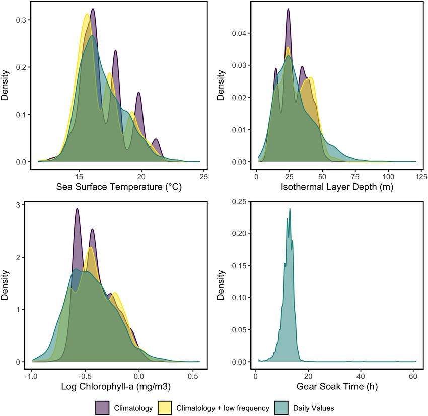
Figure 1. Map of the California Current System showing observed and decomposed sea surface temperature (SST) for two example days, 1
November 2007 (A–D), and 1 November 2015 (E–H). Swordfish catch locations aggregated to the nearest 0.5 degrees are shown, with the
red polygon indicating 95% of the catch data (core fishing zone; top left). Time-series plots (I and J) show the spatially-averaged observed
and decomposed sea surface temperature from 1998 to 2016, and were smoothed for illustrative purposes. Decomposition separated sea
surface temperature into three component parts: a monthly climatology, a low frequency signal capturing interannual variability, and a high
frequency signal capturing the remaining variability on sub-annual timescales.

features such as fronts and eddies, is commonly included               a negative binomial family and log link function, with fishing
when developing and predicting SDMs, in a forecasting sense            trip included as a random effect (using bs = ‘re’). Including
this component is unlikely to be predictable except at very            fishing trip as a random effect removed temporal autocorrela-
short lead times. Thus, if an SDM derives much of its skill            tion in the model residuals, according to the ‘acf ’ function in
from the high frequency component, it is likely to not be a            the stats R package. We did not consider swordfish popula-
good candidate for forecasts.                                          tion biomass in the North Pacific in our modelling approach
                                                                       as biomass has remained relatively constant across our study
Species distribution models                                            period (ISC 2018). Environmental covariates (SST, ILD,
                                                                       Chl) were included using a thin plate regression spline, with
A total of 4162 drift gillnet sets, totaling 8788 swordfish            the number of knots (which controls the degree of non-lin-
caught (mean catch of 2.11 swordfish per set) were used to             earity) not pre-specified. Gear soak time (h) was also included
build swordfish SDMs. Here we model swordfish catch per                as a smoother to account for variability in catch relating to
unit effort as a function of the environment. Swordfish catch          the duration of each set.
was modelled as a function of the environment using a gen-                 Three SDMs were built to partition the relative influence
eralized additive mixed model (GAMM), using the mgcv R                 of decomposed environmental covariates on model predic-
package (ver. 1.8-33; Wood 2017). GAMMs were fitted with               tive performance. The first SDM included only the monthly

4
climatologies of each environmental covariate. The second         discrimination, calibration and precision) were each averaged.
SDM included the sum of the monthly climatology and low           Second, models were trained on all data from 1998 to 2013,
frequency anomalies for each environmental covariate (i.e.        and tested against data from 2014 to 2016 when a severe
only the high frequency component was removed). The third         marine heatwave occurred in the CCS. This out-of-sample
SDM was built with the raw model output for each environ-         cross-validation approach tests how well models perform
mental covariate (i.e. including the monthly climatology, low     under novel environmental conditions (Muhling et al. 2020).
frequency and high frequency components). The three SDMs          The four measures of predictive performance described above
thus incrementally increased the temporal resolution of envi-     were then calculated. For all out-of-sample predictions, the
ronmental predictors and allowed us to partition the predic-      fishing trip random effect was excluded and soak time was
tive performance of SDMs into climatological, low frequency       fixed at 12 h (the mean of observed effort).
and high frequency environmental processes. We did not
assess the three decomposed environmental covariates indi-        Model evaluation: swordfish catch anomalies
vidually as the low and high frequency anomalies were not
individually capable of describing spatially-explicit swordfish   We then assessed the ability of the three SDMs to predict
catch. SST and ILD were correlated in the monthly clima-          swordfish catch anomalies in the core fishing zone, where
tology-only SDM and the interpretation of their response          95% of drift gillnet swordfish catch was observed from 1998
curves should be treated with caution. Environmental covari-      to 2016 (Fig. 1). We examined catch anomalies rather than
ates in the other two SDMs were not correlated.                   absolute catches to remove the influence of long-term average
                                                                  catch, and focus on the ability of models to predict changes
Model evaluation: mean catch and distribution                     in catch as a function of environmental change, a neces-
                                                                  sary step toward making accurate predictions under climate
The explanatory power and predictive performance of               change. For example, using anomalies we can assess whether
each swordfish SDM was evaluated using a series of met-           November in a given year has higher or lower catch than the
rics appropriate to the integer response variable to assess       average November, rather than whether more fish are gen-
model fit, bias and performance. Goodness-of-fit was com-         erally caught in November than December. While assessing
pared among models using Akaike’s information criterion,          model performance based on anomalies is standard practice
explained deviance (%) and r-squared. Model bias was              in climate and weather forecasting, it is less common in spe-
assessed using the slope and intercept of a linear regression     cies distribution modelling (Tommasi et al. 2017). However,
of observed and fitted abundance values. Model predictive         examining anomalies is a critical analytical step when predict-
performance was assessed using metrics of model accuracy,         ing climate change impacts, as the goal is to capture diver-
discrimination power, calibration and precision of predic-        gence from the climatological state. Here, examining catch
tions (Norberg et al. 2019). Specifically, accuracy measures      anomalies was an effective way to quantitatively assess the
the degree of proximity between the predicted and true            added value of including low and high frequency environ-
value. Discrimination power considers how well predictions        mental variability in swordfish catch models.
discern observed trends, but does not consider the absolute           To calculate swordfish catch anomalies, we first predicted
match between predicted and observed values. Calibration is       swordfish catch (number per 12 h set) in each model SDM
the statistical consistency between distributional predictions    for every day from 1998 to 2016. Predictions and observa-
and observed values, such as the proportion of observed val-      tions were limited to the core fishing zone (Fig. 1) where
ues that fall within a model’s confidence interval. Precision     95% of drift gillnet swordfish catch was observed during that
measures the width of the predictive distribution. For accu-      period. We then averaged observed and predicted swordfish
racy, calibration and precision, smaller values indicate better   catch in this core fishing zone for 1) each month in the fish-
performance. Model accuracy was determined by the root            ing season (September–January), and 2) across four spatial
mean square error between observed and predicted values.          resolutions (0.5°, 1°, 2°, and the entire core fishing zone).
Discrimination power was determined as the Spearman cor-          For both predicted and observed catch, catch anomalies were
relation coefficient between observed and predicted values.       created by first calculating a climatology of monthly sword-
Calibration was determined by finding the absolute differ-        fish catch (1998–2016), then finding the catch difference
ence between 0.5 and the proportion of predictions that fall      between each month and its monthly climatological value.
within the 50% prediction interval (i.e. the interval within          Predicted and observed anomalies for each month were
which 50% of future observations would fall) of each model        compared using two metrics. The first was Pearson correla-
(Norberg et al. 2019). Precision was determined by the stan-      tion coefficients between predicted and observed anomalies,
dard deviation of predictions that fall within the 50% predic-    with significance assessed using the test statistic, r. The sec-
tion interval (Norberg et al. 2019).                              ond was the probabilistic accuracy of the upper tercile (66%)
   These measures of model performance were assessed              of swordfish catch (Spillman and Hobday 2014). This met-
through two types of cross-validation. First, models were         ric calculates the proportion of a correct yes/no prediction
trained on a random subset of 75% of the data and tested          of swordfish catch anomalies, where a ‘correct yes’ is when
against the remaining 25%. This was repeated 10 times, and        predicted and observed catch anomalies both lie within the
the four measures of model predictive performance (accuracy,      upper tercile, and a ‘correct no’ is the opposite. Accuracy is

                                                                                                                                 5
then calculated as the sum of ‘correct yes’ and ‘correct no’, Supporting information). Given the persistence of this event,
divided by the total number of predictions (Spillman and its signal was most pronounced in the low-frequency time-
Hobday 2014, Tommasi et al. 2017). Probabilistic accuracy series, which exhibited anomalously warm water, low chloro-
ranges between 0 and 1, with values greater than 0.56 better phyll and shallow isothermal layer depths (Fig. 1, Supporting
than chance (Spillman and Hobday 2014). information).
Results Species distribution models
Decomposed environmental data Spatially-explicit predictions of swordfish catch in the core
fishing zone varied substantially depending on which scales
Decomposing environmental data into three temporal com- of decomposed environmental covariates were included. The
ponents (monthly climatology, low frequency and high fre- SDM using daily values highlighted more fine-scale oceano-
quency) highlighted both spatial and temporal trends in the graphic features relative to the SDM that included only the
structure of environmental variation. The monthly clima- monthly climatology (Fig. 2). The SDM that included both
tology revealed strong spatial gradients in ocean variables, the monthly climatology and low frequency components
including a cross-shore gradient in chlorophyll and a latitu- highlighted some of the same features as the daily values
dinal gradient in SST, while the low frequency signal showed model, with both of these models showing large differences
persistent and often widespread anomalies. In contrast, the in the distribution of swordfish catch between the two exam-
high frequency signal isolated ephemeral features such as ple years (2000 and 2015; Fig. 2). These differences amongst
fronts and eddies (Fig. 1). Time-series of all environmental SDMs emerge partly as a result of different ranges of envi-
covariates (SST, ILD, Chl) showed that the marine heatwave ronmental data available for model fitting (Fig. 3, Supporting
from 2014 to 2016 was distinct from other years (Fig. 1, information). SDMs built from the daily values see a larger
Figure 2. Predicted swordfish catch (number caught per 12 h set) from each species distribution model for two example days, 1 November
2007 (top row) and 2015 (bottom row).
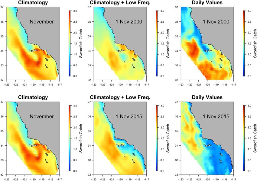
6Figure 3. Frequency distribution of environmental covariates at swordfish catch locations temporally decomposed into their component
parts (color). Covariates were used in species distribution modelling, with gear soak time consistent across all models so only one color is
shown.
range of environmental data than the two other SDMs, for Model evaluation: swordfish catch anomalies
which temporal smoothing reduces extreme values of each
predictor (e.g. deeper ILD, warmer SST and higher chl) Swordfish catch anomalies indicate whether more or less
(Fig. 3, Supporting information). swordfish are caught relative to the long-term average for
a given time and place (positive and negative anomalies,
respectively). While the SDM built on environmental cli-
Model evaluation: mean catch and distribution matologies had no ability to predict anomalous swordfish
catch, we found that the models including low and high
We found only minor differences in model fit and perfor- frequency environmental variability were able to accurately
mance among the three swordfish SDMs. Generally, there predict swordfish catch anomalies over multiple spatial scales
were incremental improvements in model fit, bias and per- (Fig. 4, Supporting information). Differences in performance
formance as the temporal resolution of decomposed environ- between the monthly climatology + low frequency SDM and
mental predictors increased from the climatological SDM to the daily values SDM were minor, with variation in per-
the climatological plus low frequency SDM to the daily val- formance attributed to the month and spatial resolution of
ues SDM (Table 1). However, there were no meaningful dif- predictions (Fig. 4). The first performance metric, Pearson
ferences among the SDMs for the four performance metrics correlation coefficient, indicates the discriminatory power of
(discrimination, accuracy, calibration and precision). This predictions. That is, when a large anomaly is observed do we
pattern generally held when cross-validating SDMs against also predict a large anomaly? Our results show that the dis-
marine heatwave years (2014–2016; Table 1). The minor dif- criminatory power was highest in the daily values model, and
ferences among SDMs indicate that most of the predictive peaked at a 2° spatial resolution. The second performance
performance of the models is derived from the monthly cli- metric, probabilistic accuracy, indicates how well we can pre-
matology of environmental covariates. dict an anomaly regardless of the magnitude of that anomaly.
7Table 1. Summary of species distribution model fit (AIC, % explained deviance and R2), bias (gradient and intercept) and model performance
(discrimination, accuracy, calibration, precision) metrics for each decomposed model (monthly climatology, monthly climatology and low
frequency, and daily values). Colors indicate the best performing model (green), to the worst performing model (red) and in between (yel-
low). Model performance metrics were completed for models trained on all years (1998–2016) and cross-validated 10 times using a random
75%/25% split, with mean (± SE) shown. Metrics were also completed for models trained on a subset of years (1998–2013) and tested on
marine heatwave years (2014–2016).
Monthly climatology Climatology + low frequency Daily values
Trained on 1998–2016
AIC 14 510 14 509 14 478
Explained deviance (%) 48.5 48.7 49.3
R2 0.37 0.376 0.373
Slope 1.587 1.569 1.488
Intercept −0.270 −0.200 −0.079
Discrimination: Mean correlation coefficient (SE) 0.352 (0.006) 0.336 (0.006) 0.334 (0.006)
Accuracy: Mean root mean square error (SE) 2.907 (0.05) 2.926 (0.05) 2.926 (0.05)
Calibration: proportion of predictions within 50% 0.297 (0.034) 0.370 (0.035) 0.288 (0.024)
prediction interval
Precision: SD of predictions within 50% prediction 0.516 (0.02) 0.537 (0.02) 0.495 (0.01)
interval
Trained on 1998–2013
AIC 13 759 13 746 13 713
Explained deviance (%) 49 50 50
R2 0.373 0.381 0.38
Gradient 1.629 1.592 1.508
Intercept −0.293 −0.211 −0.085
Discrimination: Mean correlation coefficient (SE) 0.219 0.288 0.248
Accuracy: Mean root mean square error (SE) 3.122 3.043 3.014
Calibration: |p < 0.05| 0.366 0.382 0.140
Precision: SD of predictions within 50% prediction 0.325 0.463 0.524
interval
Both the low and high frequency models had the same ability environmental and ecological scales of predictability. In con-
to differentiate the occurrence of an anomaly, and this was trast, higher frequency environmental variability (e.g. specific
consistent across the four spatial resolutions that were tested times and locations of oceanographic features such as eddies)
(Fig. 4). These results indicate that swordfish SDMs were not is not predictable on climate timescales, but its relatively
only capable of predicting anomalous catch, but that most small contribution to SDM predictive performance in our
of the predictability of anomalous catch came from the low- study suggests this lack of predictability may not be a hin-
frequency environmental component. drance to predicting and projecting species distributions.
Decomposing the environmental drivers of animal dis-
tributions allowed us to incrementally assess each compo-
Discussion nent’s role in predicting swordfish catch and distribution.
The environment will influence animal movements and
The redistribution of biodiversity as a response to climate behavior across multiple spatial and temporal scales, and
variability and change has driven the need for accurate and thus an animal’s observed location represents the integra-
precise predictions of animal distributions, but has also tion of multiple scales of variation. Animal migrations and
exposed the challenges and complexities of using correla- seasonal movements may be cued to the monthly climatol-
tive models to represent multiple, multi-scale, responses of ogy as it reflects long-term phenological patterns of resource
animals to their environment. Here, we temporally decom- availability (Bauer et al. 2011, Winkler et al. 2014), while
posed environmental information to better understand how finer-scale movements and behavior may be more closely
component signals influence the distributions of swordfish, linked to dynamic environmental cues that signal local prey
a highly mobile marine predator. We found that our abil- enhancement (Scales et al. 2014, Abrahms et al. 2018). By
ity to predict swordfish distribution and catch was driven partitioning temporal scales of environmental variability,
predominantly by a combination of climatological and low our results contribute to understanding the mechanisms
frequency environmental signals. When focusing on devia- that structure species responses to the environment at mul-
tions from historical mean swordfish catch due to anomalous tiple scales. Here, the monthly climatology of environ-
environmental conditions, the low frequency component mental covariates was likely a good predictor of swordfish
was the dominant source of predictive skill. This timescale distributions because swordfish exhibit seasonality and some
is consistent with the target timescales of climate forecasts degree of site fidelity in their movements (Sepulveda et al.
and projections, indicating a promising match between the 2020). The incremental improvement in model predictive
8Figure 4. Average observed swordfish catch (maps) and predictive performance for modeled swordfish catch anomalies, with predictions
averaged over four spatial resolutions (0.5°, 1°, 2° and the entire region). Anomaly correlation coefficients (middle column) and probabi-
listic accuracy (right column) are shown for each month for the daily values species distribution model (blue circles), the monthly climatol-
ogy plus low frequency model (yellow triangles), and the monthly climatological model (purple squares). Blue crosses and yellow stars
indicate significance of the correlation coefficients (p < 0.05). The horizontal black line at 0.56 indicates the minimum level of probabilistic
accuracy, with values below this no better than random. Correlation coefficients for the monthly climatology are 0 and not shown.
performance with the addition of the low-frequency com- longer-term environmental conditions. The spatial scale of
ponent reflects the high mobility of swordfish, which allows fisheries effort and ROMS data was ~10 km, so we were
them to move in response to local and interannual variabil- unable to resolve biological and environmental processes at
ity. However, we found that the addition of high frequency finer scales at which swordfish respond to their immediate
environmental variability to these broader scale signals did environment. Our decomposition approach systematically
not meaningfully improve predictability, although it did identified the temporal scales of swordfish predictability, but
increase SDM explanatory power. This may be because this approach would not be necessary if a swordfish SDMs
fine-scale swordfish distributions are driven by prey distri- purpose was to explain habitat use and historical distribu-
butions and foraging behavior at depth, and we therefore tion – as is the case in most SDM purposes (Araújo et al.
might not expect swordfish to respond to high frequency 2019). Under such purposes, using the daily values of envi-
(e.g. ephemeral) environmental features in surface waters. ronmental covariates would likely maximize the explanatory
In other words, our results suggest a swordfish was caught power of models (Scales et al. 2017a).
at a location not because of its immediate ‘here and now’ Our analysis adds to a growing body of literature that
environment, but rather due predominantly to broader and indicates that the utility of climatological information is
9becoming increasingly degraded given the accelerating pace species distribution modelling, assessing skill based on anom-
of global change and non-stationarity in ecosystem responses alies is common practice in climate and weather studies: for
(Zimmermann et al. 2009, Zurell et al. 2009, Scales et al. example, a model is not assessed by whether it can predict
2017a, Muhling et al. 2020). Indeed, much of the climate if summer is on average warmer than winter, but whether a
velocity literature argues that local environmental condi- given summer is warmer or colder than the average summer.
tions drive species movements and population range shifts These skill metrics are becoming more common in ecologi-
(Pinsky et al. 2013, Sunday et al. 2015, Brito-Morales et al. cal forecasting applications (Hobday et al. 2016). We suggest
2018). Here we show evidence that a combination of clima- that in a prediction context, the suite of SDM performance
tological and low-frequency environmental processes govern metrics should distinguish skill in predicting distribution
our ability to accurately predict the distribution and move- anomalies from skill in predicting climatological patterns.
ments of a highly mobile predator species. We might expect Much of the explanatory power in our SDM of swordfish
this combination of inter-annual and long-term timescales in the CCS came from the environmental monthly climatol-
of environmental variation to provide predictability of spe- ogy, but the monthly climatology itself cannot be used to
cies distributions for many mobile marine and terrestrial predict deviations from mean species distributions. Thus, the
species that exhibit spatial shifts in response to environmen- ability of low- and to a lesser degree high-frequency environ-
tal change. However, the low-frequency component of pre- mental variability to enable skillful predictions of anomalous
dictability may be less important for species with high site species distributions is a key result of our study; indeed, it
fidelity, particularly terrestrial species that are able to exploit indicates the feasibility of forecasting species distribution
microclimates in response to adverse environmental condi- changes on both short (seasonal) and long-term (climate
tions (e.g. thermal refugia; Pinsky et al. 2019). For species change) timescales. For swordfish specifically, we might
that can exploit microclimates, high frequency environmen- expect climate change to delay the arrival of cooler waters
tal variability (in addition to static variables, such as substrate to the southern California Bight and subsequently shift the
type) may play a larger role in predicting species distribution typical peak period of catch (Sep–Nov) to later in the win-
than seen here for the pelagic swordfish. However, we should ter season. The implications of such a shift for the fishery
acknowledge that the spatial scale being examined will have could be drastic without appropriate mitigation or adapta-
a large influence on the relative importance of component tion. For example, temporal shifts in key swordfish fishing
signals. For example, on a global scale a species distribution months may be impacted by poor weather (i.e. late winter
might be best predicted by long-term mean conditions, but and spring storms) and overlap with other seasonal fisher-
on a local scale (e.g. meters) the high frequency components ies (e.g. gear switching; Frawley et al. 2020) which would
should be more important in describing species distribu- likely have an economic impact on this fishery (Smith et al.
tions and habitat use. Testing our temporal decomposition 2020). Application of a seasonal forecasting product to pre-
approach on other species and on different spatial scales dict whether a swordfish fishing season will be typical or
would further help to elucidate the spatiotemporal scales of anomalous may help to improve the resilience and capacity
predictability in species distributions. of fishers in response to climate change. Our results show
The metrics of predictive performance that we used to the potential for a skillful seasonal forecast for this sword-
compare across abundance-based SDMs are well known and fish fishery, as the low-frequency temperature variability that
frequently used (Norberg et al. 2019), yet showed inconsis- drives swordfish distribution anomalies in the CCS has been
tent results and in certain cases indicated only minor differ- shown to be skillfully forecast by global climate prediction
ences across SDMs (Table 1). Such variability and minor systems (Jacox et al. 2019). Additionally, we demonstrate
improvement are consistent with similar studies that have a straightforward approach to decompose and evaluate the
compared SDMs built with climatological and extreme event drivers of ecological predictability which could be applied in
data (e.g. heatwaves and droughts; Morán-Ordóñez et al. other study systems as a precursor to ecological forecasting.
2018), and local weather data (Zimmermann et al. 2009). Ecological forecasting requires identifying a particular
Zimmermann et al. (2009) in particular noted that the pri- metric that is accurately predictable and relevant to the fore-
mary impact of including local weather conditions in SDMs cast end-user (Jacox et al. 2020). Our results indicate that
was a minimization of over- and underprediction, with only we could accurately predict swordfish catch anomalies dur-
modest improvements in area under the receiver operating ing a historical testing period, but the two metrics used to
characteristic curve (AUC) (a standard evaluation metric of assess predictive ability did not show consistent patterns
binomial SDMs). However, an important distinction should across SDMs or spatial resolution of catch anomalies. This
be made between the standard SDM performance metrics disparity is likely a function of how fisher behavior can influ-
(Table 1) and assessment of skill for predicting anomalous ence fisheries data. For example, when environmental con-
species distributions. The climatological environmental data ditions become more favorable for positive catch anomalies,
have by definition no ability to predict anomalous distribu- this doesn’t necessarily mean that fishing effort or catch will
tions. Since the goal of many prediction or projection analyses increase. Other factors, like spatiotemporal management
is to capture changes from the climatological state, it is criti- zones, historical fisher knowledge and weather can all impact
cal in this context to assess model skill for predicting anoma- where and when fishers fish (Frawley et al. 2020, Smith et al.
lies of species distribution and catch. While uncommon in 2020). In light of remaining uncertainties in swordfish
10distribution predictions, along with relevant scales for man- (supporting). Heather Welch: Data curation (supporting);
agement action, it may be more pragmatic to forecast species Writing – review and editing (supporting). Michael G.
distributions probabilistically (e.g. with tercile classification; Jacox: Formal analysis (supporting); Funding acquisition
Fig. 4) than deterministically (e.g. with exact values of habi- (lead); Methodology (supporting); Project administration
tat suitability or catch). It is important to understand these (lead); Writing – review and editing (supporting).
limitations of predictability for ecological forecasting, and
ongoing work could further explore predictability through
retrospective skill testing (Hobday et al. 2016, Brodie et al.
2017). References
Abecassis, M. et al. 2012. Modeling swordfish daytime vertical
Conclusion habitat in the North Pacific Ocean from pop-up archival tags.
– Mar. Ecol. Prog. Ser. 452: 219–236.
Understanding the factors that promote accurate prediction Abrahms, B. et al. 2018. Mesoscale activity facilitates energy gain
of species distributions in response to environmental change in a top predator. – Proc. R. Soc. B 285: 20181101.
is vital for informing climate-ready and proactive ecosystem Abrahms, B. et al. 2019a. Memory and resource tracking drive
management. Here, we identify the temporal scales of envi- blue whale migrations. – Proc. Natl Acad. Sci. USA 116:
ronmental variability that provide predictive skill for the dis- 5582–5587.
tribution of a mobile marine predator, distinguishing their Abrahms, B. et al. 2019b. Dynamic ensemble models to predict
ability to explain historical mean distributions from their distributions and anthropogenic risk exposure for highly mobile
ability to predict distribution anomalies. In doing so, we species. – Divers. Distrib. 25: 1182–1193.
Aikens, E. O. et al. 2017. The greenscape shapes surfing of
highlight how both long-term and interannual environmen-
resource waves in a large migratory herbivore. – Ecol. Lett.
tal variability help to structure the distributions of a mobile 20: 741–750.
marine predator. Understanding the scales that provide skill Araújo, M. B. et al. 2019. Standards for distribution models in
for predicting species responses to the environment gives biodiversity assessments. – Sci. Adv. 5: eaat4858.
confidence in our ability to accurately predict species redis- Bauer, S. et al. 2011. Cues and decision rules in animal migration.
tributions, and to know which responses are likely unpredict- – In: Milner-Guland, E. J. et al. (eds), Animal migration: a
able, under future climate change. synthesis. Oxford Univ. Press, pp. 68– 87.
Becker, E. A. et al. 2018. Predicting cetacean abundance and dis-
Data availability statement tribution in a changing climate. – Divers. Distrib. 25:
626–643.
NOAA fisheries observer data for the drift gillnet fishery is not Becker, E. A. et al. 2019. Predicting cetacean abundance and dis-
publicly available. Contact authors directly to request access. tribution in a changing climate. – Divers. Distrib. 25:
626–643.
Block, B. A. et al. 2011. Tracking apex marine predator movements
in a dynamic ocean. – Nature 475: 86–90.
Acknowledgements – We thank John Childers and Yuhong Gu for Boersma, P. D. and Rebstock, G. A. 2014. Climate change increases
assistance with the NMFS observer program data. reproductive failure in Magellanic penguins. – PLoS One 9:
Funding – Funding was provided by NOAA’s Modeling, Analysis, e85602.
Predictions and Projections MAPP Program (NA17OAR4310108); Bond, N. A. et al. 2015. Causes and impacts of the 2014 warm
NOAA’s Coastal and Ocean Climate Application COCA Program anomaly in the NE Pacific. – Geophys. Res. Lett. 42:
(NA17OAR4310268); the NOAA Fisheries Office of Science and 3414–3420.
Technology, and NOAA’s Integrated Ecosystem Assessment Program. Boustany, A. M. et al. 2010. Movements of Pacific bluefin tuna
Thunnus orientalis in the eastern North Pacific revealed with
Author contributions archival tags. – Progr. Oceanogr. 86: 94–104.
Brito-Morales, I. et al. 2018. Climate velocity can inform conserva-
Stephanie Brodie: Conceptualization (lead); Data cura- tion in a warming world. – Trends Ecol. Evol. 33: 441–457.
tion (lead); Formal analysis (lead); Investigation (lead); Brodie, S. J. et al. 2020. Tradeoffs in covariate selection for species
Methodology (lead); Visualization (lead); Writing – origi- distribution models: a methodological comparison. – Ecogra-
nal draft (lead); Writing – review and editing (lead). Briana phy 43: 11–24.
Abrahms: Writing – original draft (supporting); Writing Brodie, S. et al. 2017. Seasonal forecasting of dolphinfish distribu-
– review and editing (supporting). Steven J. Bograd: tion in eastern Australia to aid recreational fishers and manag-
Investigation (supporting); Writing – review and editing ers. – Deep Sea Res. Part II Top. Stud. Oceanogr. 140:
(supporting). Gemma Carroll: Investigation (support- 222–229.
Brodie, S. et al. 2018. Integrating dynamic subsurface habitat
ing); Writing – review and editing (supporting). Elliott
metrics into species distribution models. – Front. Mar. Sci. 5:
L. Hazen: Investigation (supporting); Writing – review 219.
and editing (supporting). Barbara A. Muhling: Writing Caretta, J. V. et al. 2004. Estimates of marine mammal, sea turtle
– review and editing (supporting). Mercedes Pozo Buil: and seabird mortality in the California drift gillnet fishery for
Writing – review and editing (supporting). James A. Smith: swordfish and thresher shark, 1996–2002. – Mar. Fish. Rev. 66:
Methodology (supporting); Writing – review and editing 21–30.
11Cavole, L. et al. 2016. Biological impacts of the 2013–2015 warm- Jacox, M. G. et al. 2020. Seasonal-to-interannual prediction of
water anomaly in the northeast Pacific winners, losers and the North American coastal marine ecosystems: forecast methods,
future. – Oceanography 29: 273–285. mechanisms of predictability and priority developments. –
Checkley Jr., D. M. and Barth, J. A. 2009. Patterns and processes Progr. Oceanogr. 183: 102307.
in the California Current System. – Progr. Oceanogr. 83: 49–64. Kharouba, H. M. et al. 2018. Global shifts in the phenological
Descamps, S. et al. 2015. Demographic effects of extreme weather synchrony of species interactions over recent decades. – Proc.
events: snow storms, breeding success and population growth Natl Acad. Sci. USA 115: 5211–5216.
rate in a long-lived A ntarctic seabird. – Ecol. Evol. 5: Leising, A. W. et al. 2015. State of the California Current
314–325. 2014–2015: impacts of the warm-water ‘Blob’. – Calif Coop
Dewar, H. et al. 2011. Movements and behaviors of swordfish in Oceanic Fish Investig Rep 56: 31–68.
the Atlantic and Pacific Oceans examined using pop-up satellite Morán-Ordóñez, A. et al. 2018. Modelling species responses to
archival tags. – Fish. Oceanogr. 20: 219–241. extreme weather provides new insights into constraints on range
Dietze, M. C. et al. 2018. Iterative near-term ecological forecasting: and likely climate change impacts for Australian mammals. –
needs, opportunities and challenges. – Proc. Natl Acad. Sci. Ecography 41: 308–320.
USA 115: 1424–1432. Mueller, T. et al. 2011. How landscape dynamics link individual-to
Edwards, M. and Richardson, A. J. 2004. Impact of climate change population-level movement patterns: a multispecies comparison
on marine pelagic phenology and trophic mismatch. – Nature of ungulate relocation data. – Global Ecol. Biogeogr. 20: 683–694.
430: 881–884. Muhling, B. A. et al. 2020. Predictability of species distributions
Elith, J. and Leathwick, J. R. 2009. Species distribution models: deteriorates under novel environmental conditions in the Cali-
ecological explanation and prediction across space and time. – fornia Current System. – Front. Mar. Sci. 7:589.
Annu. Rev. Ecol. Evol. Syst. 40: 677–697. Neveu, E. et al. 2016. An historical analysis of the California Cur-
Franklin, J. 2010. Moving beyond static species distribution mod- rent circulation using ROMS 4D-Var: system configuration and
els in support of conservation biogeography. – Divers. Distrib. diagnostics. – Ocean Model. Online 99: 133–151.
16: 321–330. Norberg, A. et al. 2019. A comprehensive evaluation of predictive
Frawley, T. H. et al. 2020. Changes to the structure and function performance of 33 species distribution models at species and
of an albacore fishery reveal shifting social–ecological realities community levels. – Ecol. Monogr. 89: e01370.
for Pacific Northwest fishermen. – Fish Fish. 22: 280–297. Parmesan, C. and Yohe, G. 2003. A globally coherent fingerprint
Grall, C. et al. 1983. Distribution, relative abundance and season- of climate change impacts across natural systems. – Nature 421:
ality of swordfish larvae. – Trans. Am. Fish. Soc. 112: 235–246. 37–42.
Guisan, A. and Thuiller, W. 2005. Predicting species distribution: Payne, M. R. et al. 2017. Lessons from the first generation of
offering more than simple habitat models. – Ecol. Lett. 8: marine ecological forecast products. – Front. Mar. Sci. 4: 289.
993–1009. Perry, A. L. et al. 2005. Climate change and distribution shifts in
Hanan, D. A. et al. 1993. The California drift gill net fishery for marine fishes. – Science 308: 1912–1915.
sharks and swordfish, 1981–1982 through 1990–1991. – State Pinsky, M. L. et al. 2013. Marine taxa track local climate velocities.
of California, Resources Agency, Dept of Fish and Game. – Science 341: 1239–1242.
Hazen, E. L. et al. 2013. Predicted habitat shifts of Pacific top pred- Pinsky, M. L. et al. 2019. Greater vulnerability to warming of
ators in a changing climate. – Nat. Clim. Change 3: 234–238. marine versus terrestrial ectotherms. – Nature 569: 108–111.
Hazen, E. L. et al. 2018. A dynamic ocean management tool to Poloczanska, E. S. et al. 2013. Global imprint of climate change on
reduce bycatch and support sustainable fisheries. – Sci. Adv. 4: marine life. – Nat. Clim. Change 3: 919–925.
eaar3001. Reside, A. E. et al. 2010. Weather, not climate, defines distributions
Hickey, B. M. 1979. The California Current system – hypotheses of vagile bird species. – PLoS One 5: e13569.
and facts. – Progr. Oceanogr. 8: 191–279. Robinson, N. M. et al. 2017. A systematic review of marine-based
Hobday, A. J. et al. 2016. Seasonal forecasting for decision support species distribution models (SDMs) with recommendations for
in marine fisheries and aquaculture. – Fish. Oceanogr. 25: 45–56. best practice. – Front. Mar. Sci. 4: 421.
Hobday, A. J. et al. 2018. A framework for combining seasonal Scales, K. L. et al. 2014. On the Front Line: frontal zones as prior-
forecasts and climate projections to aid risk management for ity at-sea conservation areas for mobile marine vertebrates. – J.
fisheries and aquaculture. – Front. Mar. Sci. 5: 137. Appl. Ecol. 51: 1575–1583.
Horton, T. W. et al. 2020. Multi-decadal humpback whale migra- Scales, K. L. et al. 2017a. Scale of inference: on the sensitivity of
tory route fidelity despite oceanographic and geomagnetic habitat models for wide-ranging marine predators to the resolu-
change. – Front. Mar. Sci. 7: 414. tion of environmental data. – Ecography 40: 210–220.
Huyer, A. 1983. Coastal upwelling in the California Current sys- Scales, K. L. et al. 2017b. Fit to predict? Eco-informatics for pre-
tem. – Progr. Oceanogr. 12: 259–284. dicting the catchability of a pelagic fish in near real time. – Ecol.
ISC 2018. ISC Billfish Working Group. Stock assessment for Appl. 27: 2313–2329.
swordfish Xiphias gladius in the Western and Central North Sepulveda, C. A. et al. 2010. Fine-scale movements of the swordfish
Pacific Ocean through 2016. – Western and central Pacific Fish- Xiphias gladius in the southern California Bight. – Fish. Ocean-
eries Commission, . ogr. 19: 279–289.
Jacox, M. G. et al. 2016. Impacts of the 2015–2016 El Niño on Sepulveda, C. A. et al. 2020. Insights into the horizontal move-
the California Current System: early assessment and compari- ments, migration patterns and stock affiliation of California
son to past events. – Geophys. Res. Lett. 43: 7072–7080. swordfish. – Fish. Oceanogr. 29: 152–168.
Jacox, M. G. et al. 2019. On the skill of seasonal sea surface tem- Sepulveda, C. A. et al. 2018. Movements and behaviors of sword-
perature forecasts in the California Current System and its con- fish Xiphias gladius in the United States Pacific Leatherback
nection to ENSO variability. – Clim. Dyn. 53: 7519–7533. Conservation Area. – Fish. Oceanogr. 27: 381–394.
12You can also read