Numerical integration schemes for the equations of motion, constants of motion, control of stability, accuracy - Ari Paavo Seitsonen - cecam
←
→
Page content transcription
If your browser does not render page correctly, please read the page content below
Numerical integration schemes for the equations of
 motion, constants of motion, control of stability,
                     accuracy

                 Ari Paavo Seitsonen
               École Normale Supérieure

            CECAM QM/MM School, Lausanne
                 April 8th -12th , 2019

     apsi                                  QM/MM 2019   1 / 53
Molecular dynamics

apsi                        QM/MM 2019   2 / 53
Molecular dynamics

   Propagation of Newton’s equation of motion (with discrete equations of
   motion)
                             FI = MI a = MI R̈I

   Alternative derivation from the Lagrange formalism:
                                 N
                              X  1
                    L RN , ṘN =     MI Ṙ2I − U RN ,

                                   2
                                   I=1

   U is the interaction potential between the particles. The Euler-Lagrange
   equation
                                   d ∂L       ∂L
                                            =
                                   dt ∂ ṘI   ∂RI

   Most common algorithm: Verlet algorithm (in a few variations)

        apsi                                                  QM/MM 2019   3 / 53
Verlet algorithm: Velocity Verlet
discretisation of Newton’s equation of motion
MI R̈I = FI
i) Propagate ionic positions RI (t) according to
2
(∆t)
RI (t + ∆t) = RI (t) + ∆t vI (t) + FI (t)
2MI
ii) Evaluate forces FI (t + ∆t) at RI (t + ∆t)
iii) Update velocities
∆t
vI (t + ∆t) = vI (t) + [FI (t) + FI (t + ∆t)]
2MI
apsi QM/MM 2019 4 / 53Velocity Verlet: Advantages
Other algorithms provides can have better short time stability and allow larger
time steps, but . . .
simple and efficient; needs only forces, no higher energy derivatives
still correct up to and including third order, (∆t)3
explicitly time reversible
sympletic: conserves volume in phase space
superior long time stability (energy conservation) of the Verlet algorithm
apsi QM/MM 2019 5 / 53Velocity Verlet: Choice of time step
The time step is in general chosen as large as possible . . .
“Possible” = stable dynamics = energy conserved; or, drift in energy
acceptable
Rule of thumb: 6-10 times smaller than the fastest period in the system;
otherwise sampling of that mode is impossible
Time step can be changed during simulation(!)
apsi QM/MM 2019 6 / 53Velocity Verlet: Choice of time step
AlCl3 dimer
Example of a good/bad choice of time step
Highest vibrational frequency 595 cm−1 ⇒ period T = 56 fs
Divergence between δt = 400..500 atu = 9.6-12.0 fs ≈ 1/5 T
apsi QM/MM 2019 7 / 53Equations of motion: Alternative derivation
Propagation methods
Define phase space vector Γ = (x, p) and commutator
∂A ∂H ∂A ∂H
{A, H} = −
∂x ∂p ∂p ∂x
Hamilton’s equations of motion:
dΓ
= {Γ, H}
dt
Define L̂ so that
i L̂Γ = {Γ, H}
Γ̇ = i L̂Γ ⇒
Γ(t) = ei L̂t Γ(0)
Such formalism has been used by Mark Tuckerman et al to derive new
integrators
apsi QM/MM 2019 8 / 53Tricks
Simulated annealing
Multiple time scales / RESPA
Periodic boundary conditions
Ewald summation
Thermodynamic integration
Cell lists etc
apsi QM/MM 2019 9 / 53Molecular dynamics: Summary
Molecular dynamics can be used to perform real-time dynamics in
atomistic systems
Maximum time step ∆t ≈ 1 fs (highest ionic frequency
2000 − 3000 cm−1 )
Temperature can be controlled via rescaling – (initial) equilibration – and
thermostats (e. g. Nosé-Hoover thermostat chains) for NVT ensemble
Constraints can be used to pose restrictions on the atoms
They can be used to direct reactions, however in complicated
(potential/free) energy landscapes they might not yield the correct
reaction path (in reasonable simulation time, at least)
Metadynamics looks like a promising method for finding reaction paths
and (potential/free) energy surfaces
apsi QM/MM 2019 10 / 53Ab initio molecular dynamics apsi QM/MM 2019 11 / 53
Realistic MD simulations

                          MI R̈I = −∇R E ({RJ })

   Classical molecular dynamics: E ({RJ }) given e. g. by pair potentials
   How about estimating E ({RJ }) directly from electronic structure
   method?
                                       dE
   What is needed is −∇R E ({RJ }) = − dRI

        apsi                                                  QM/MM 2019    12 / 53
Classical vs MD simulations
When is electronic structure needed explicitly, when is classical
treatment sufficient?
I Chemical reactions: Breaking and creation of chemical bonds
I Changing coordination
I Changing type of interaction
I Difficult chemistry of elements
Combination of both: QM/MM
apsi QM/MM 2019 13 / 53Born-Oppenheimer
molecular dynamics
apsi QM/MM 2019 14 / 53Born-Oppenheimer Ansatz
Separate the total wave function to quickly varying electronic and slowly
varying ionic wave function:
NBO
X
ΦBO ({ri } , {RI } ; t) = Ψ̃k ({ri } , {RI }) χ̃ ({RI } ; t)
k =0
Leads to a Schrödinger-like equation for the electrons and a Newton-like
equation for the ions (after some assumptions for the ionic wave
function):
He Ψ̃k ({ri } , {RI }) = e
E{RI}
Ψ̃k ({ri } , {RI })
MI R̈I = FI
Electrons always at the ground state when observed by the ions
Usually valid, however there are several cases when this Ansatz fails
apsi QM/MM 2019 15 / 53Born-Oppenheimer MD
Lagrangean
N
X 1
MI Ṙ2I − min EKS {ψi } , RN
LBO R, Ṙ =
2 {ψi }
I=1
equations of motion:
d
MI R̈I = −∇R EKS Ψ, RN = − min EKS {ψi } , RN
dRI {ψi }
If the right-hand side can be evaluated analytically it can be plugged
directly to the Verlet algorithm
apsi QM/MM 2019 16 / 53Forces in BOMD
What is needed is
d
min EKS {ψi } , RN
−
dRI {ψi }
with the constraint that the orbitals remains orthonormal; this is achieved
using Lagrange multipliers in the Lagrangean
X
EKS = EKS + Λij (hψi | ψj i − δij )
ij
Forces
dEKS ∂EKS ∂ X ∂ hψi |
∂EKS +
X X
= + Λij hψi | ψj i + Λij |ψj i
dRI ∂RI ∂RI ∂RI ∂ hψi |
ij ij j
When |ψi i optimal
∂EKS X ∂
FKS (RI ) = − + Λij hψi | ψj i
∂RI ∂RI
ij
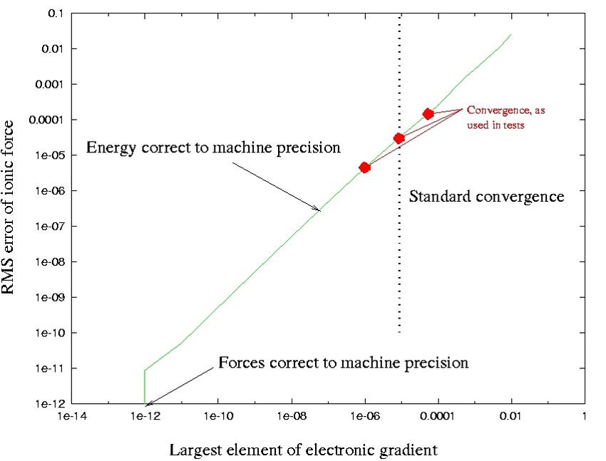
apsi QM/MM 2019 17 / 53BOMD: Error in forces
The error in the forces depends on the convergence criterion set for the
electronic structure in BOMD:
apsi QM/MM 2019 18 / 53BOMD: Observations
The energy needs to be minimal in order to estimate the forces
The accuracy of the forces depends on the level of self-consistency
Thus a competition between accuracy and computational cost
Constant of motion:
I NVE:
N
X 1
MI Ṙ2I + min EKS {ψi } , RN
2 {ψi }
I=1
I NVT:
N
X 1 1
2
MI Ṙ2I + min EKS {ψi } , RN + Qs ṡ2 + gkB T ln(s)
2s {ψi } 2
I=1
apsi QM/MM 2019 19 / 53Car-Parrinello method apsi QM/MM 2019 20 / 53
Car-Parrinello method
Roberto Car & Michele Parrinello, Physical Review Letters 55, 2471 (1985)
    They postulated Langangean
                                                M
                          n o                 X 1 D           E
                LCP {ψi } , ψ̇i ; R, Ṙ     =       µ ψ̇i | ψ̇i
                                                  2
                                                i=1

                                                −min{ψi } EKS {ψi } , RN


                                                    N
                                                    X 1
                                                +             MI Ṙ2I
                                                          2
                                                    I=1

    Reminder: EKS contains the Lagrange multipliers for orthonormality of
    orbitals
    Fictitious or fake dynamics of electrons
    µ = fictitious mass or inertia parametre
    Simultaneous dynamics of ions and electrons

         apsi                                                           QM/MM 2019   21 / 53
Car-Parrinello method: Equations of motion
Euler-Lagrange equations
d ∂LCP ∂LCP
D =
dt ∂ ψ̇ ∂ hψi |
i
d ∂LCP ∂LCP
D =
dt ∂ Ṙ ∂ hRI |
I
Equations of motion
∂EKS X
µψ̈i = − + Λij |ψj i
∂ hψi |
j
∂EKS X ∂
MI R̈I = − + Λij hψi | ψj i
∂RI ∂RI
ij
apsi QM/MM 2019 22 / 53Car-Parrinello method: Simultaneous dynamics
Unified Approach for Molecular Dynamics and Density-Functional
Theory
Electronic and ionic structure evolve simultaneously
Whereas in BOMD first the electronic structure is optimised, then the
ions are moved
apsi QM/MM 2019 23 / 53Car-Parrinello method: Constant of motion
Constant of motion
M N
X 1 D E X 1
Econserved = µ ψ̇i | ψ̇i + EKS {ψi } , RN + MI Ṙ2I
2 2
i=1 I=1
Note: instantaneous value of EKS {ψi } , RN , not minimum
Thus no need to optimise the orbitals at each step
apsi QM/MM 2019 24 / 53Magic Car-Parrinello method
Does the Car-Parrinello method yield physical results even if the orbitals
are not at the Born-Oppenheimer surface?
I Yes — provided that the electronic and ionic degrees of freedom
remain adiabatically separated and the electrons close to the
Born-Oppenheimer surface
I Why? — dynamics of the electrons is artificial, or unphysical and
thus has to average out during the time scale of ionic movement
Another way of viewing: The electrons are slightly above the BO surface
but remain there and average out the effects on the ions (to be
considered with care)
apsi QM/MM 2019 25 / 53Adiabatic separation
Pastore, Smargiassi & Buda, PRA 1991
Vibrational spectra of electrons and ions do not overlap:
Triangle = highest ionic frequency
apsi
Z ∞ XD E QM/MM 2019 26 / 53Adiabatic separation
Thus there’s no efficient mechanism for exchange of energies: The two
subsystems are adiabatically decoupled
Triangle = highest ionic frequency
Z ∞ XD E
e
f (ω) = cos (ωt) ψ̇i (t) ψ̇i (0) dt
t=0 i
apsi QM/MM 2019 27 / 53Constant of motion
Physical and conserved energy:
N
X 1
Ephysical = EKS {ψi } , RN + MI Ṙ2I
2
I=1
M N
X 1 D E X 1
Econserved = µ ψ̇i | ψ̇i + EKS {ψi } , RN + MI Ṙ2I
2 2
i=1 I=1
= Ekin,fict + Ephysical
PM D E
The difference, Ekin,fict = i=1 12 µ ψ̇i | ψ̇i , must thus correlate with the
changes in the physical energy
apsi QM/MM 2019 28 / 53Constant of motion: Conservation of energy
Model system: Two-atom Si-fcc
Energy components
Ekin,f
apsi QM/MM 2019 29 / 53Deviation from Born-Oppenheimer surface
Deviation of forces in CP dynamics from the true BO forces small
and/but oscillating
Fx (Si) Fx,CP (Si)-Fx,BO (Si)
apsi QM/MM 2019 30 / 53Control of adiabacity
Harmonic analysis: s
2 (εi − εj )
ωije =
µ
εi occupied, εj unoccupied (virtual) orbitals
Lowest frequency s
e Egap
ωmin ∝
µ
Highest frequency s
e Ecut
ωmax ∝
µ
Thus maximum possible time step
r
µ
(∆t e )max ∝
Ecut
apsi QM/MM 2019 31 / 53Control of adiabacity
Lowest frequency has to be well above ionic frequencies
s
e Egap
ωmin ∝
µ
Highest frequency limits the maximum possible time step
s r
e Ecut e µ
ωmax ∝ (∆t )max ∝
µ Ecut
If ∆t fixed and µ chosen
I too small: Electrons too light and adiabacity will be lost
I too large: Electrons too heavy, the slowest electronic motion starts
to overlap with the ionic frequencies and adiabacity will be lost
apsi QM/MM 2019 32 / 53Loss of adiabacity: Difficult cases
Vacancy in hot 64-atom Si cell
apsi QM/MM 2019 33 / 53Loss of adiabacity: Difficult cases
Sn2 : Degeneracy of HOMO and LUMO at short distances
apsi QM/MM 2019 34 / 53Analysis of adiabacity: Simplified model
Two-level, two-electron model
Wave function
θ θ
ψ= cos Φ1 + sin Φ2
2 2
θ is the electronic degree of freedom
Constant gap Opening-closing gap G
apsi QM/MM 2019 35 / 53Zero or small electronic gaps: Thermostatted
electrons
One way to (try to) overcome the problem in coupling of electronic and
ionic dynamics is to thermostat also the electrons [Blöchl & Parrinello,
PRB 1992]
Thus electrons cannot heat up; if they try to, thermostat will adsorb the
excess heat
Target fictitious kinetic energy Ekin,0 instead of temperature
“Mass” of thermostat to be selected appropriately:
I Too light: Adiabacity violated (electrons may heat up)
I Too heavy: Ions dragged excessively
Please remember: The conserved quantity changed
apsi QM/MM 2019 36 / 53Thermostat on electrons
Example: Aluminium
Dependence of the heat transfer on the choice of Ekin,0 in solid Al
apsi QM/MM 2019 37 / 53Thermostat on electrons: Does it help?
64 atoms of molten aluminium
(a): Without thermostat
(b): With thermostat
apsi QM/MM 2019 38 / 53Thermostat on electrons: Does it work?
Check: Radial pair correlation function
I Solid line: CP-MD with thermostat
I Dashed line: Calculations by Jacucci et al
apsi QM/MM 2019 39 / 53Rescaling of ionic masses
The fictitious electronic mass exerts an extra “mass” on the ions and
thereby modifies the equations of motion:
X ∂φi ∂φi
MI R̈I = FI + µ R̈I
∂r ∂r
i∈I
The new equations of motion:
(MI + dMI ) R̈I = FI
where
2 I
µE dMI =
3 kin
is an unphysical “mass”, or drag, due to the fictitious kinetics of the
electrons
Example: Vibrations in water molecule
mode harmonic BOMD 50 100 200 400 dM/M [%]
bend 1548 1543 1539 1535 1529 1514 0.95×10⁻³ µ
sym. 3515 3508 3494 3478 3449 3388 1.81×10⁻³ µ
asym. 3621 3616 3600 3585 3556 3498 1.71×10⁻³ µ
apsi QM/MM 2019 40 / 53Orthonormality constraints
Equations of motion
∂EKS X
µψ̈i = − + Λij |ψj i
∂ hψi |
j
In principle differential equations, however after discretisation difference
equations (Verlet algorithm)
Therefore the algorithm for the constraints Λij depends on the integration
method
apsi QM/MM 2019 41 / 53Orthonormality constraints: RATTLE
Define
∆t 2 p ∆t 2 v
Xij = Λ Yij = Λ C wf coefficients
2µ ij 2µ ij
Equations of type
1
XX† + XB + B† X† = I − A Q + Q†
Y=
2
∗
P
A, B, Q of type Aij = G cGi cGj
Solve iteratively:
1h i
X(n+1) = I − A + X(n) (I − B) + (I − B) X(n) − X(n) X(n)
2
apsi QM/MM 2019 42 / 53CP tricks apsi QM/MM 2019 43 / 53
Car-Parrinello method for structural optimisation:
Simulated annealing
   In larger molecules or crystals the structural optimisation might be
   difficult, especially the closer to the minimum one is
   CPMD can be used to perform the optimisation by simulated annealing:
   Rescaling the (atomic and possibly also electronic) velocities:

                                    Ṙ0I = αṘI

   Easy to incorporate into the velocity Verlet algorithm
   Optimised structure when all velocities (temperature) are ≈ 0
     I   Check by calculating the ionic forces
   The ionic masses are “unphysical”: Select to “flatten” the vibrational
   spectrum (e. g. high mass on hydrogens)
   Faster convergence due to the “global” optimisation

         apsi                                                  QM/MM 2019   44 / 53
Basis set dependent mass
µ can be chosen to be dependent on the basis set:
µ
0 , H (G, G) ≤ α
µ (G) =
1
(µ/α) G2 + V (G, G) , H (G, G) < α
2
Kind of “pre-conditioning” of the equation of motion
Allows for larger time step
However, leads to much larger corrections on the ionic frequencies and
no analytical formula can be used
apsi QM/MM 2019 45 / 53CP & BO apsi QM/MM 2019 46 / 53
Car-Parrinello vs Born-Oppenheimer dynamics
 Born-Oppenheimer MD                Car-Parrinello MD
 Exactly on BO surface              Always slightly off BO surface

 ∆t ≈ ionic time scales,            ∆t  ionic time scales,
 maximum time step possible         (much) shorter time step necessary

 Expensive minimisation             Orthogonalisation only,
 at each MD step                    less expensive per MD step

 Not stable against deviations      Stable against deviations
 from BO surface                    from BO surface
 ⇒ Energy/temperature drift,
 thermostatting of ions necessary

 Same machinery in zero-gap         Thermostatting of electrons
 systems                            to prevent energy exchange

 Many applications in solids        Used in liquids, ...

               apsi                                                      QM/MM 2019   47 / 53
CP vs BO
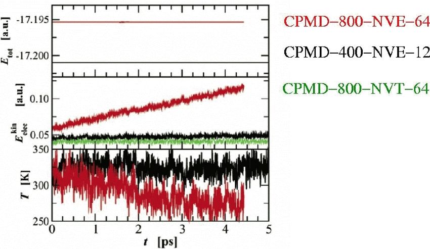
apsi QM/MM 2019 48 / 53CP vs BO: Stability
apsi QM/MM 2019 49 / 53BO: Error in forces
The error in the forces depends on the convergence criterion set for the
electronic structure in BOMD:
apsi QM/MM 2019 50 / 53CP vs BO: Liquid water
Effect of µ: Too large value leads to loss of adiabacity
Thermostatting the electrons recovers the correct behaviour
apsi QM/MM 2019 51 / 53CP vs BO: Liquid water: Results
The radial distribution functions are correct and independent of the
method used
apsi QM/MM 2019 52 / 53Car-Parrinello method: Summary
Car-Parrinello method can yield very stable dynamical trajectories,
provided the electrons and ions are adiabatically decoupled
The method is best suited for e. g. liquids and large molecules with an
electronic gap
The speed of the method is comparable or faster than using
Born-Oppenheimer dynamics — and still more accurate (i. e. stable)
apsi QM/MM 2019 53 / 53You can also read