Numerical investigation of effects of incisor angle on production of sibilant /s/ - Nature
←
→
Page content transcription
If your browser does not render page correctly, please read the page content below
www.nature.com/scientificreports
OPEN Numerical investigation of effects
of incisor angle on production
of sibilant /s/
HsuehJui Lu1,2, Tsukasa Yoshinaga3, ChungGang Li1,2*, Kazunori Nozaki4, Akiyoshi Iida3 &
Makoto Tsubokura1,2
The effects of the inclination angle of the incisor on the speech production of the fricative consonant
/s/ was investigated using an implicit compressible flow solver. The hierarchical structure grid was
applied to reduce the grid generation time for the vocal tract geometry. The airflow and sound during
the pronunciation of /s/ were simulated using the adaptively switched time stepping scheme, and the
angle of the incisor in the vocal tract was changed from normal position up to 30°. The results showed
that increasing the incisor angle affected the flow configuration and moved the location of the high
turbulence intensity region thereby decreased the amplitudes of the sound in the frequency range
from 8 to 12 kHz. Performing the Fourier transform on the velocity fluctuation, we found that the
position of large magnitudes of the velocity at 10 kHz shifted toward the lip outlet when the incisor
angle was increased. In addition, separate acoustic simulations showed that the shift in the potential
sound source position decreased the far-field sound amplitudes above 8 kHz. These results provide the
underlying insights necessary to design dental prostheses for the production of sibilant fricatives.
Fricative consonants are speech sounds that are produced via turbulent flow in the vocal tract. It is known that
the central incisor position and angle affect speech production, especially that of the fricative consonant /s/ 1–5.
During the articulation of /s/, a constricted flow channel (sibilant groove) is formed between the tongue tip and
the upper incisors. Because the /s/ sound is generated by the turbulent jet flow leaving the c onstriction6, inac-
curate formation of the constriction results in speech production difficulties for /s/.
Runte et al.1 constructed a maxillary denture, and the inclination angle of the central incisor was changed
within the range of − 30° to + 30° to investigate the influence of the angle on the production of /s/. Meanwhile,
the jaw movement during the phonation of /s/ was measured to observe the closest oral tract space with the hori-
zontal and vertical overlap of the incisors7. Hamlet et al.8 measured the tongue movement with a contact sensor
and showed the effects of dental prostheses on the timing and duration of the constriction formation of sibilant
fricatives. However, because the /s/ sound is generated by jet flow in the oral tract, the detailed mechanisms of
the effects of dental prostheses on the observed sound changes are unclear.
The production mechanisms in the absence of articulatory dysfunction have been investigated by modeling
the vocal tract geometry. Shadle9 proposed a simplified vocal tract model for fricative consonants and investigated
the effects of teeth-like obstacle positions on the generated sounds. In addition, numerical flow simulations were
applied to a simplified model and the effects of geometrical differences on the turbulent jet flow and its sound
sources were e xamined10,11.
To further investigate the airflow associated with the production of /s/ and its source characteristics in an
actual oral tract, a vocal tract replica was constructed from computational tomography (CT) images and the
flow and sound generated in the replica were measured using a microphone and an anemometer12. A numerical
flow simulation of a realistic vocal tract geometry revealed that the aeroacoustic sound source is located near
the upper and lower incisor s urfaces13.
Recently, both turbulent flow for /s/ and the sound generated by the vocal tract geometry were predicted via
numerical simulations using high-performance computing resources14–17. These simulations revealed that the
sound source is located downstream of the upper and lower incisors and that the acoustic characteristics of /s/ are
1
Computational Fluid Dynamics Laboratory, Department of Computational Science, Graduate School of
System Informatics, Kobe University, 1‑1 Rokkodai, Nada‑ku, Kobe 657‑8501, Japan. 2Complex Phenomena
Unified Simulation Research Team, RIKEN, Advanced Institute for Computational Science, Kobe 650‑0047,
Japan. 3Toyohashi University of Technology, 1‑1 Hibarigaoka, Tempaku‑cho, Toyohashi, Aichi 441‑8580,
Japan. 4Osaka University Dental Hospital, 1‑1 Yamadaoka, Suita, Osaka 565‑0871, Japan. *email: cgli@
aquamarine.kobe-u.ac.jp
Scientific Reports | (2021) 11:16720 | https://doi.org/10.1038/s41598-021-96173-2 1
Vol.:(0123456789)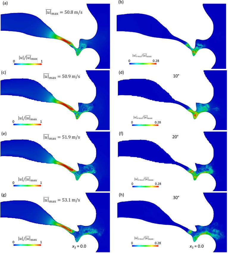
www.nature.com/scientificreports/
formed by the geometry downstream of the constriction. However, the effects of geometrical differences resulting
from dental prosthesis, e.g., the incisor positions and angles, on the flow and sound generation are still unclear.
Therefore, in this study, we conducted numerical flow simulations of the vocal tract geometry of /s/ at dif-
ferent incisor angles to examine the origin of sound changes using the inclination angles of the incisor reported
by Runte1. To explore the cause of the sound changes, both the airflow for /s/ and the sound in the vocal tract
geometry were predicted using numerical simulations solving the three-dimensional compressible Navier–Stokes
equation18–20. One difficulty with numerical flow simulations is maintaining high-quality computational grids
for the complex flow channel in the vocal tract geometry. To reduce the grid generation time for the vocal tract
geometry, we applied the hierarchical structure grid21 in the simulations. By further developing the proposed
methodology, this simulation technology will enable us to predict the effects of dental prostheses on the produc-
tion of sibilant fricatives for patients prior to prosthetic surgery.
Methods
Vocal tract geometry. To simulate the phenomena involved in the pronunciation of /s/, the geometry
of a vocal tract replica was constructed from CT images12. The subject was a 32-year-old Japanese male who
self-reported no speech disorders with a normal dentition of angle class I, without inter-teeth spacing. The CT
images were taken while the subject sustained the pronunciation of /s/ for 9.6 s without vowel context, and
the image resolution was 0.1 × 0.1 × 0.1 mm3. The surfaces of the vocal tract geometry were extracted based on
brightness values using the software itk-SNAP22. Since the resolution of the CT scan is 0.1 mm and the tips of
the incisors were slightly smoothed through the vocal tract extraction from the CT scan, we have confirmed that
the extracted vocal tract geometry reproduced the subject’s pronunciation of /s/ up to 14 kHz by constructing an
oral replica12. The ethics committee of the graduate school of Osaka University certified this study (H26-E39).
Figure 1a shows the vocal tract geometry, including the throat, tongue, hard palate, incisors, and lips. The x1
is defined as the anterior–posterior direction; the x2 is defined as the inferior–superior direction; x3 is defined
as the transverse direction. The initial inclination angle of the incisor to the maxillary plane was 108° for this
subject. For the inclined cases, the variation from + 10° to + 30° was resulted in 118° to 138° based on this origi-
nal incisor angle, and the region of the inclination incisor is marked in red color (− 10 mm < x3 < 10 mm). The
geometries from the top and side views are shown in Fig. 1b,c, respectively. We confirmed that the exclusion of
the upstream vocal tract geometry on the simulation of /s/ was negligible for the main acoustic characteristics
of /s/14. According to R unte1, by comparing the sound of /s/ generated by the human subject with the subject’s
vocal tract replica made of plaster using a 3D printer, the frequency characteristics of /s/ were produced up to
16 kHz with the maximum discrepancy of 8 dB. It indicates that the solid wall condition is valid to investigate
the sound mechanisms.
To investigate the effect of the inclination angle of the upper incisor, the incisor position
(− 17.7 mm < x1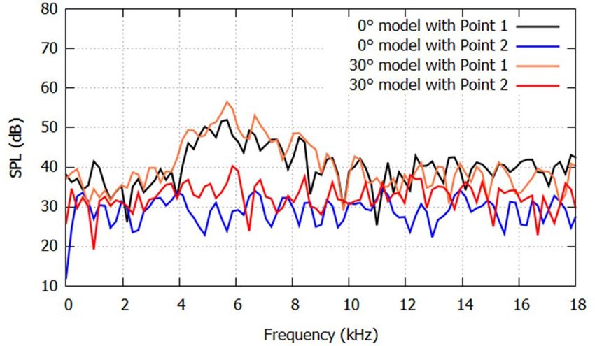
www.nature.com/scientificreports/
Figure 1. (a) Vocal tract geometry for pronouncing /s/. (b) Top and (c) side views of the vocal tract.
∂ui ∂uj 2
Aij = + − (∇ · u)δij . (5)
∂xj ∂xi 3
The pressure P follows the ideal gas equation:
P = ρRT. (6)
The dynamic viscosity µ and thermal conductivity k are based on Sutherland’s law:
3
T 2 T0 + 110
µ(T) = µ0 , (7)
T0 T + 110
µ(T)γ R
k(T) = , (8)
(γ − 1) Pr
where ρ0 = 1.1842 kg/m3, µ0 = 1.85 10−5 N∙s/m2, T0 = 298.06 K, γ = 1.4, R = 287 J/kg, and the Prandtl number
(Pr) is 0.71.
To solve the three-dimensional compressible flow governed by Eq. (1), we applied the following numeri-
cal framework. The second-order-accurate implicit lower–upper symmetric Gauss–Seidel scheme (LUSGS) is
adopted for time integration. The Roe scheme with a preconditioning method and dual time stepping is applied,
and the discretized form of Eq. (1) with artificial time step Δτ is
k+1 k k+1 n n−1
Up − Up
3U − 4U + U 1 k+1 k+1
Ŵ + + F 1
1
− F 1
1
�τ 2�t �x1 i+ 2 ,j,k i− 2 ,j,k
(9)
1 k+1 k+1 1
k+1 k+1
+ F 2
1
− F 2
1
+ F 3 i,j,k+1/2 − F 3 i,j,k−1/2 = 0,
�x2 i,j+ 2 ,k i,j− 2 ,k �x3 ( ) ( )
where Г is the preconditioning matrix proposed by Weiss and S mith23, Up is the primitive form [P, u1, u2, u3, T],
τ is artificial time and t is physical times, the superscripts k and n are the iteration numbers in artificial time step
and the proceeding step of real time, respectively. The quantities associated with the artificial time term of the
(k + 1)th iteration are transferred approximately to quantities of the (n + 1)th time step in real time when the
term ∂Up /∂τ converges to zero. Then, Eq. (9) will be reduced to the original Navier–Stokes equation including
the transient term.
Finally, Eq. (1) can be rearranged as
I 3
+ Ŵ −1 M + Ŵ −1 (δx1 Akp + δx2 Bpk + δx3 Cpk ) �Up = Ŵ −1 Rk , (10)
�τ 2�t
w here M = ∂U/∂Up , Akp = ∂F1k /∂Up , Bpk = ∂F2k /∂Up , Cpk = ∂F3k /∂Up are t he f lux Jacobi an,
k k k
Rk = −(3U k − 4U n + U n−1 )/(2�t) − (δx1 F 1 + δx2 F 2 + δx3 F 3 ), and δxi is the central-difference operator.
24
To accelerate the convergence speed, Lian et al. proposed the solution-limited time stepping (SLTS) method
by adaptively adjusting the CFL number and determine Δτ in the governing equation. When adopting LUSGS
method, the estimation value ΔQest defined as
k k
|�Qest = −�τ M −1 − 3U k − 4U n + U n−1 /(2�t) − δx1 F 1 + δx2 F 2 , (11)
and ΔQref is defined as
Scientific Reports | (2021) 11:16720 | https://doi.org/10.1038/s41598-021-96173-2 3
Vol.:(0123456789)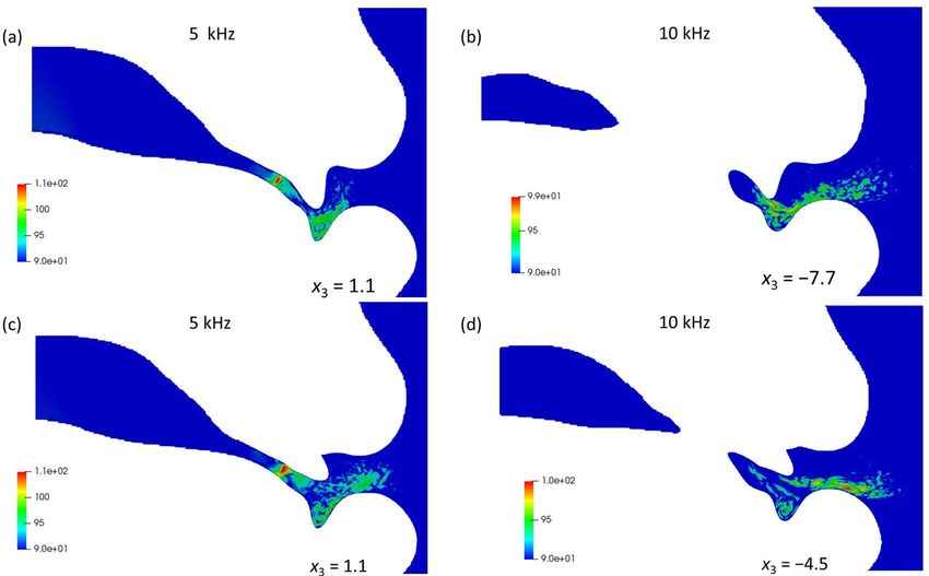
www.nature.com/scientificreports/
Figure 2. Vocal tract geometry with the incisor angle increased from the original position (0°) to 30°: (a)
original geometry with 0°; (b) modified geometry with 30°; and (c) modified geometry with the incisor angle
ranging from 0° to 30°.
� 2
u22 , �Psur , Pglobal × 10�−9
� � �
α1 × max 0.5
��× ρ u1 +
α2 × max u2 + u2 �, �Psur ×c , Vglobal × 10−9
�� 1 2 γP
(12)
�
��Qref = ,
�
α3 × max u2 + u2 , �Psur ×c , Vglobal × 10−9
�
1 2 γP
α4 × T
where ΔPsur is the maximum difference between the pressure at surrounding points and Pglobal, Vglobal denotes the
global value that ensures the reference values are always greater than 0, c is the speed of sound, and γ is the heat
capacity ratio. Equation (12) provide a criterion for determining whether the calculation is stable or not. The
factor [α1 α2 α3 α4] is the coefficient of the maximum allowable fractional change according to L ian24. Under the
SLTS method, the larger physical time step and the faster speed of convergence can be achieved. However, because
of the Newton linearization error of the term ∂Up /∂τ , SLTS method is not suitable for aeroacoustic simulations
even when the convergence criteria are satisfied. Hence, we applied the adaptively switched time stepping scheme
(ASTS)25 to reduce the computational cost and maintain the accuracy in the aeroacoustic simulation.
In the calculation of Rk on the right-hand side of Eq. (10), the terms involving Fi in Eq. (3) can be divided
into an inviscid term Finviscid, and a viscous term Fviscous, as shown below:
ρui
ρui u1 + pδi1
Finviscid = ρui u2 + pδi2 , (13)
ρu u + pδ
i 3 i3
(ρe + p)ui
0
µAi1
Fviscous = − µAi2 . (14)
µAi3
∂T
µAij uj + ∂x i
When employed the Roe scheme in Eq. (14), Finciscid term will be discretized into
1
Finviscid,i+1/2 = [FR (U) + FL (U)] + Fd , (15)
2
where Fd is the Roe dissipation term, which is composed of jumps of properties of work fluids. For the recon-
struction of FR and FL, the fifth-order monotone upstream-centered scheme for conservation laws (MUSCL)26
without a limiter function to prevent turbulent fluctuations from attenuating. Aside from the inviscid term, the
derivative terms in Aij in the viscous term of Eq. (3) are calculated using the second-order central difference. The
detail of the current framework can be found in previous study18–20.
Computational conditions. To simulate the complex geometry, e.g., a realistic human oral cavity, the
immersed boundary method with the hierarchical structure grid21 was applied for the grid spacing. As the grid
configuration, the computational domain is divided according to the hierarchical structure system proposed by
Nakahashi21. Using a hierarchical structure grid can shorten the working time required to build computational
grids and simultaneously provide better load balancing and higher performance for parallel computations.
After testing the space resolution, the minimum grid size was set as 0.05 mm around the upper incisors
to keep the accuracy of the immersed boundary around the turbulent region. To simulate the sound waves
Scientific Reports | (2021) 11:16720 | https://doi.org/10.1038/s41598-021-96173-2 4
Vol:.(1234567890)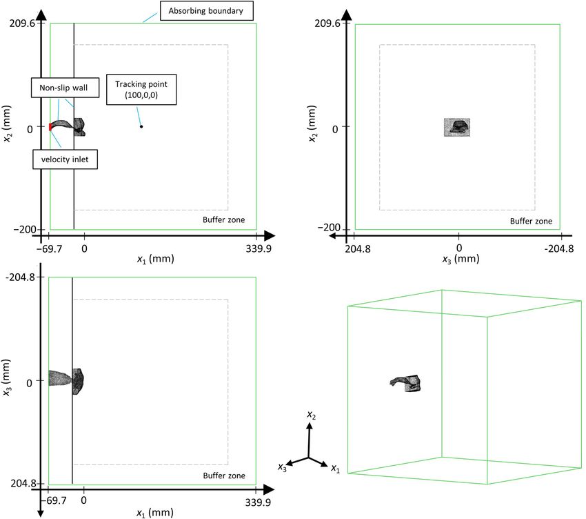
www.nature.com/scientificreports/
propagating through the lip outlet, the far-field region was set outside of the vocal tract model. The total grid
numbers of the 0–30° cases were 8.7 × 10⁷, 7.2 × 10⁷, 7.8 × 10⁷, and 6.7 × 10⁷, respectively.
The three-view diagram of overall computational domain with the boundary condition and tracking point
for the current model are shown in Fig. 3. The inlet was set to a uniform velocity condition to simulate the
pronunciation of /s/. The uniform inlet velocity was set to 1.5 m/s, which resulted in−a physiological flow rate
of 330 c m3/s 12. The Reynolds number was 5632, based on the maximum velocity (|u|max = 50.8 m/s ) inside
the oral cavity in the original geometry. To keep the flow in the computational domain from being polluted by
reflecting pressure waves, an absorbing boundary condition was used as the outlet condition. The absorbing
boundary condition used in the current study is based on JB Freund27 and extend by L i20 which is adjusted for
the low flow speed simulation. The time step was set to 10−6 s, so that the CFL number was 7.8, which fulfilled
the condition for the ASTS m ethod26. The physical time of the performed simulations was 0.015 s and required
parallel computing with 1152 cores on 32 nodes for 30 h. Table 1 summarizes the computational parameters for
the simulations. Fast Fourier transform (FFT) using the Hann window was applied to the waveforms sampled
100 mm from the lip outlet (x1 = 100 mm) to analyze the far-field sound spectrum. The FFT sampling frequency
was 50 kHz with 256 points averaged five times. The sound pressure level (SPL) was calculated based on the
reference pressure Pref = 20 × 10−6 Pa. In addition to the sound spectrum, the magnitudes of the velocity fluctua-
tions at each frequency were calculated via FFT on each grid to identify the highest contribution position for
the potential sound source23.
Results and discussion
To ascertain the accuracy of the simulation in the present framework, the result was compared with experimental
measurements. The acoustic pressure was collected 100 mm from the lip outlet (x1 = 100 mm), and the frequency
spectra of the sound was calculated via FFT, as shown in Fig. 4a. We have confirmed that the velocity magnitude
around the tracking point is small enough to be neglected, which is less than 0.05 m/s. In the experiment, the
vocal tract replica was constructed using a 3D printer (Objet30Pro, Stratasys, USA; accuracy: ± 0.1 mm) and a
constant flow was input to the model using a compressor (YC-4RS, Yaezaki, Tokyo, Japan). The sound generated
by the model was measured using a microphone (type 4939, Bruel & Kjaer, Nærum, Denmark) at a distance of
x1 = 100 mm in an anechoic chamber (with a volume of 8.1 m3). The pronunciation of /s/ was recorded with an
actual subject for 18 times of utterances. The subject sustained /s/ for 3 s without vowel context, and before the
signal was calculated via FFT, some portions of signals after the onset and before the offset of /s/ are removed.
Therefore, inclusion of the effect of the onset and offset was avoided.
The sibilant sound is characterized as a broadband noise above 4 kHz. At a frequency of 3 kHz, SPL rapidly
increased, and the first characteristic peak reached around 5 kHz. This result shows good agreement with the
measurements for the actual subject and oral replica, and the same characteristics of sibilant /s/ sound was
observed by Runte1. Accordingly, this result suggests that the present framework of the direct aeroacoustic
computation can provide aeroacoustic predictions with reasonable accuracies.
To investigate the effects of the incisor angle, the incisor angle was varied from 0° to 30°; the far-field SPL
spectra for these angles are shown in Fig. 4b. According to Runte1, the changes of incisor angle of denture led to
a different noise band range. In this study, amplitudes from 8 to 12 kHz were decreased by the increase of incisor
angle. This means that the upper boundary frequency of noise was decreased and the noise band range became
smaller with the inclined incisors. While the noise band range of 0° was approximately 4 kHz to 12 kHz, the noise
band range of 30° was 4 kHz to 8 kHz. This result is consistent with that found by Runte1. Besides, according to
Snow28, general audible frequency range for male and female speech are up to 7 kHz, and 9 kHz, respectively,
and the characteristic peak of the sibilant sound at around 4 kHz was observed for all teeth angles. Therefore,
the sounds generated by all the cases can be characterized and recognized as sibilant fricative /s/. However, the
decreasing amplitudes in the frequency range 8 kHz to 12 kHz might affect−the recognition of the sound.
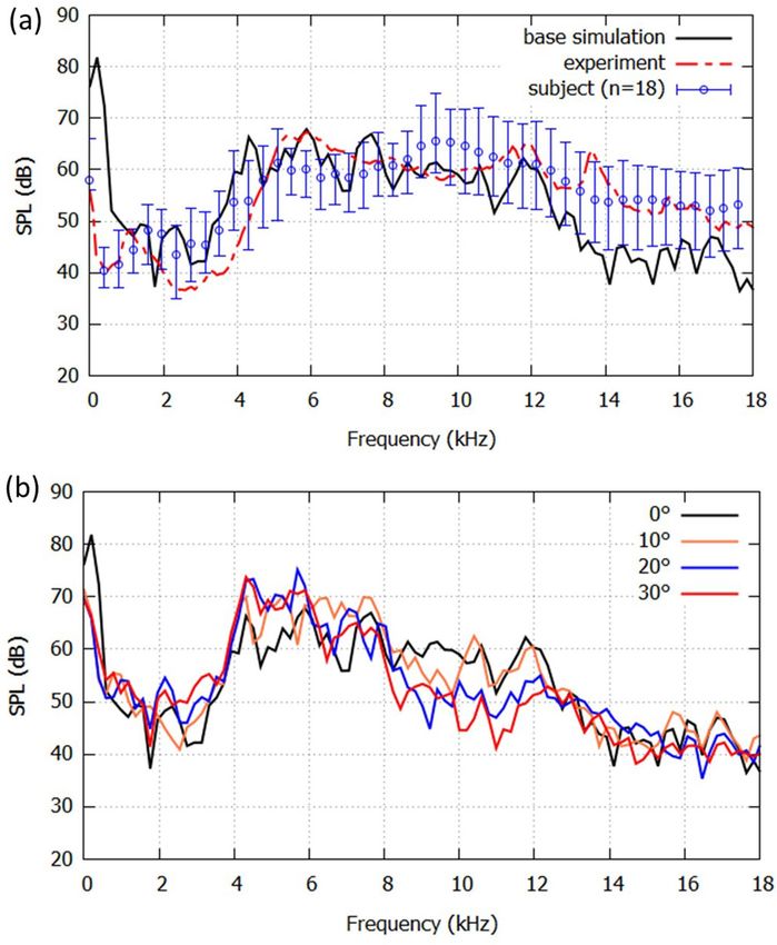
Figure 5 shows the normalized instantaneous
− velocity magnitude |u|/|u|max and root mean square (RMS)
value of the velocity fluctuations |u|rms /|u|max from the 0° to 30° models on the mid-sagittal plane (x3 = 0). As
shown in Fig. 5a,c,e,g, the instantaneous velocities of all cases are accelerated at the narrow channel between the
tongue and the hard palate (the sibilant groove) (− 25 mm < x1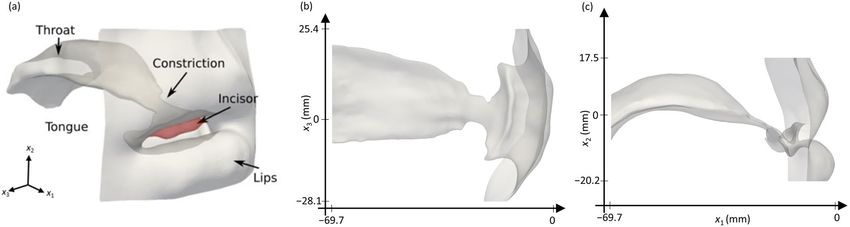
www.nature.com/scientificreports/
Figure 3. The three-view diagram of overall computational domain of the current model.
emerged at this position. Conversely, the maximum value at 10 kHz appeared at the cavity between the teeth
and the lower lip, which is at the position (49.1, − 8.4, − 7.7). This corresponds to the exit of the jet flow being the
gap between the teeth. The magnitudes of the velocity fluctuations for the 30° model at 5 kHz (x3 = 1.1 mm) and
10 kHz (x3 = − 4.5 mm) are shown in Fig. 6c,d. The maximum value for 5 kHz appeared at the exit of the sibilant
groove, which is the same as the position for the 0° model at 5 kHz. These results indicate that the velocity fluc-
tuations downstream of the constriction formed the characteristic peak at 5 kHz for both the 0° and 30° models.
Conversely, at 10 kHz, the jet flow of the 30° model passed along the surface of the incisor and the maximum
value of the velocity fluctuations appeared above the lower lip, which was at the position (58.5, − 7.7, − 4.5).
To determine the relationship between the positions of the velocity fluctuations, i.e., the assumed aeroacoustic
sound sources, and the far-field SPL spectra, instead of the base simulation with constant velocity inlet from the
throat, the acoustic simulations with acoustic monopole sources were conducted for the 0° and 30° cases. In the
previous acoustic studies, monopole to quadrupole sound sources were used to emulate the sound generated
by the turbulent fl ow29,30. Therefore, for the simplicity, the monopole sources composed of white noise were
applied in the current study at Point 1 (49.1, − 8.4, − 7.7) and Point 2 (58.5, − 7.7, − 4.5), which corresponded to
the positions of maximum velocity fluctuations at 10 kHz for both models.
A comparison of the far-field sound spectra in Fig. 7 shows an obvious amplitude difference between the two
sound source positions in the frequency range of 4–8 kHz. When the acoustic source is located at Point 1, SPL
shows the characteristics of the sibilant sound for both the 0° and 30° models. Conversely, SPL generated by the
sound source at Point 2 consisted of a broad noise with amplitudes lower than those generated at Point 1. This is
because the acoustic source at Point 1 was located inside the modeled vocal tract geometry and the sound wave
was resonated by the front oral cavity. The distance from the glosso-palatal constriction to anterior lip surface
Scientific Reports | (2021) 11:16720 | https://doi.org/10.1038/s41598-021-96173-2 6
Vol:.(1234567890)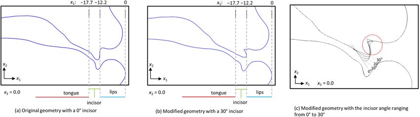
www.nature.com/scientificreports/
Size of the largest cell (mm) 1.6
Size of the smallest cell (mm) 0.05
Computational domain (mm3) 409.6 × 409.6 × 409.6
Inlet velocity (m/s) 1.5
Re 5632
Time step (s) 10−6
Physical time (s) 0.015
Table 1. Computational parameters of the 0° model.
Figure 4. (a) Sound pressure level (SPL) spectrum of the base simulation (0°, solid black line) and
measurements of the printed replica (dashed red line) and the average value of an actual subject for 18
recordings (blue circles). The error bars denote the range for 18 repeated recordings. (b) The predicted SPL
spectra with incisor angles from 0° to 30°.
was 1.39 cm, which was close to the quarter of wavelength around 6 kHz. Therefore, SPL around 6 kHz was larger
and the sound generated by Point 1 still had the characteristics of the sibilant sound in the far field. In contrast,
because the acoustic source at Point 2 was located almost entirely outside of the vocal tract, the source did not
Scientific Reports | (2021) 11:16720 | https://doi.org/10.1038/s41598-021-96173-2 7
Vol.:(0123456789)www.nature.com/scientificreports/
Figure 5. (a,c,e,g) Normalized instantaneous velocity magnitude and (b,d,f,h) root mean square (RMS) of the
velocity fluctuations at t = 0.015 s for the (a,b) 0°, (c,d) 10°, (e,f) 20°, and (g,h) 30° models.
couple strongly with the resonator, and no significant sound could be caught in the entire frequency range at the
far-field. For this reason, the far-field SPL around 10 kHz was smaller in the 30° case. Consequently, the shift in
the aeroacoustic source position affected the resonance of the sound waves and influenced the far-field SPLs of /s/.
These findings and the framework of the current simulation model can clarify the effects of geometrical dif-
ferences resulting from dental prosthesis, e.g., the incisor positions and angles, on the flow as well as the sound
generation. Besides, it can be used to help design dental prostheses at the same time predict the outcomes of
surgical procedures for the production of sibilant fricatives.
Conclusions
To investigate the effect of the inclination angle of the incisor on the speech production of the sibilant /s/,
numerical flow simulations of a vocal tract geometry with different incisor angles was conducted. On the basis
of the far-field SPL spectrum, increasing the incisor angle from 0° to 30° had no influence on the characteristic
peak of the sibilant sound at 4 kHz. However, increasing the incisor angle reduced the amplitude of the sound
in the frequency range from 8 to 12 kHz. In the flow field, the turbulence intensity kept the same level and the
maximum velocity occurred at the sibilant groove in all cases, while the high RMS value region moved from
the cavity between the teeth and the lower lip to the tip of the lower lip when the inclination angle increased.
Scientific Reports | (2021) 11:16720 | https://doi.org/10.1038/s41598-021-96173-2 8
Vol:.(1234567890)www.nature.com/scientificreports/
Figure 6. Fast Fourier transforms of the velocity fluctuations at (a,c) 5 kHz and (b,d) 10 kHz for the (a,b) 0°
and (c,d) 30° models.
Figure 7. SPL spectra for the 0° and 30° models predicted for the monopole acoustic sources at Point 1
(0.049, − 0.0084, − 0.0077) and Point 2 (0.0585, − 0.0077, − 0.0045).
By conducting acoustic simulations with a monopole source at the potential sound source positions of the 0°
and 30° cases, we found that the acoustic source position affects the resonance of the sound wave and influences
the far-field SPL spectrum. Specifically, if the sound source position was located closer to the exit of the vocal
tract, i.e., the lips, the source didn’t couple strongly with the resonator, and no significant frequency could be
caught at far-field. Because the flow channel downstream of the sibilant groove became wider when the incisor
angle was increasing from 0° to 30°, the large velocity fluctuation region was shifted and the amplitude of the
far-field sound around 10 kHz was reduced. Consequently, the slight change of the geometry affected less to the
turbulent intensity, but changed the flow configuration and shifted the position of the potential sound source,
Scientific Reports | (2021) 11:16720 | https://doi.org/10.1038/s41598-021-96173-2 9
Vol.:(0123456789)www.nature.com/scientificreports/
thereby influenced the performance on the acoustics field. These results provide the underlying insights neces-
sary to design dental prostheses for the production of sibilant fricatives.
Data availability
The datasets generated during and/or analysed during the current study are available from the corresponding
author on reasonable request.
Received: 9 March 2021; Accepted: 2 August 2021
References
1. Runte, C. et al. The influence of maxillary central incisor position in complete dentures on /s/ sound production. J. Prosthet. Dent.
85(5), 485 (2001).
2. Lee, A. S., Whitehill, T. L., Ciocca, V. & Samman, N. Acoustic and perceptual analysis of the sibilant sound /s/ before and after
orthognathic surgery. J. Oral Maxillofac. Surg. 60(4), 364 (2002).
3. Liu, R. et al. Association of incisal overlaps with /s/ sound and mandibular speech movement characteristics. Am. J. Orthod.
Dentofacial Orthop. 155(6), 851 (2019).
4. Fonteyne, E. et al. Speech evaluation during maxillary mini-dental implant overdenture treatment: A prospective study. J. Oral
Rehabil. 46(12), 1151 (2019).
5. Hu, S., Wan, J., Duan, L. & Chen, J. Influence of pontic design on speech with an anterior fixed dental prosthesis: A clinical study
and finite element analysis. J. Prosthet. Dent. https://doi.org/10.1016/j.prosdent.2020.06.040 (2020).
6. Stevens, K. N. Airflow and turbulence noise for fricative and stop consonants: Static considerations. J. Acoust. Soc. Am. 50(4B),
1180 (1971).
7. Burnett, C. A. & Clifford, T. J. Closest speaking space during the production of sibilant sounds and its value in establishing the
vertical dimension of occlusion. J. Dent. Res. 72(6), 964 (1993).
8. Hamlet, S. L., Cullison, B. L. & Stone, M. L. Physiological control of sibilant duration: Insights afforded by speech compensation
to dental prostheses. J. Acoust. Soc. Am. 65(5), 1276 (1979).
9. Shadle, C. H. The acoustics of fricative consonants, Ph.D. Thesis, Massachusetts Institute of Technology (1985).
10. Van Hirtum, A., Grandchamp, X., Pelorson, X., Nozaki, K. & Shimojo, S. Les and “in vitro” experimental validation of flow around
a teeth-shaped obstacle. Int. J. Appl. Mech. 2(02), 265 (2010).
11. Cisonni, J., Nozaki, K., Van Hirtum, A., Grandchamp, X. & Wada, S. Numerical simulation of the influence of the orifice aperture
on the flow around a teeth-shaped obstacle. Fluid Dyn. Res. 45(2), 025505 (2013).
12. Nozaki, K., Yoshinaga, T. & Wada, S. Sibilant /s/ simulator based on computed tomography images and dental casts. J. Dent. Res.
93(2), 207 (2014).
13. Nozaki, K. Numerical simulation of sibilant [s] using the real geometry of a human vocal tract. In High Performance Computing
on Vector Systems 2010 (eds Resch, M. et al.) 137–148 (Springer, 2010).
14. Yoshinaga, T., Nozaki, K. & Wada, S. Experimental and numerical investigation of the sound generation mechanisms of sibilant
fricatives using a simplified vocal tract model. Phys. Fluids 30(3), 035104 (2018).
15. Pont, A., Guasch, O., Baiges, J., Codina, R. & Van Hirtum, A. Computational aeroacoustics to identify sound sources in the genera-
tion of sibilant /s/. Int. J. Numer. Method Biol. 35(1), e3153 (2019).
16. Yoshinaga, T., Nozaki, K. & Wada, S. Aeroacoustic analysis on individual characteristics in sibilant fricative production. J. Acoust.
Soc. Am. 146(2), 1239 (2019).
17. Yoshinaga, T., Nozaki, K. & Iida, A. Hysteresis of aeroacoustic sound generation in the articulation of [s]. Phys. Fluids 32, 105114
(2020).
18. Li, C. G. & Tsubokura, M. An implicit turbulence model for low-Mach Roe scheme using truncated Navier-Stokes equations. J.
Comput. Phys. 345, 462 (2017).
19. Li, C. G. A compressible solver for the laminar–turbulent transition in natural convection with high temperature differences using
implicit large eddy simulation. Int. Commun. Heat Mass Transf. 117, 104721 (2020).
20. Li, C. G., Tsubokura, M., Fu, W. S., Jansson, N. & Wang, W. H. Compressible direct numerical simulation with a hybrid boundary
condition of transitional phenomena in natural convection. Int. J. Heat Mass Transf. 90, 654–664 (2015).
21. Nakahashi, K. Building-cube method for flow problems with broadband characteristic length. In Computational Fluid Dynamics
2002 (eds Armfield, S. W. et al.) 77–81 (Springer, 2003).
22. Lighthill, M. J. On sound generated aerodynamically I. General theory. Proc. R. Soc. Lond. Ser. A Math. Phys. Sci. 211(1107), 564
(1952).
23. Weiss, J. M. & Smith, W. A. Preconditioning applied to variable and constant density flows. AIAA J. 33, 2050–2057 (1995).
24. Lian, C., Xia, G. & Merkle, C. L. Solution-limited time stepping to enhance reliability in CFD applications. J. Comput. Phys. 228,
4836–4857 (2009).
25. Li, C. G., Lu, H. & Tsubokura, M. An adaptive time stepping scheme for aeroacoustic computations. In International Conference
on Flow Dynamics 2019/11 (Japan, Sendai, 2019).
26. Kim, K. H. & Kim, C. Accurate, efficient and monotonic numerical methods for multi-dimensional compressible flows Part II:
Multi-dimensional limiting process. J. Comput. Phys. 208, 570–615 (2005).
27. Freund, J. B. Proposed inflow/outflow boundary condition for direct computation of aerodynamic sound. AIAA J. 35(4), 740–742
(1997).
28. Snow, W. B. Audible frequency ranges of music, speech and noise. Bell Syst. Tech. J. 10(4), 616 (1931).
29. Yoshinaga, T., Van Hirtum, A., Nozaki, K. & Wada, S. Acoustic modeling of fricative/s/for an oral tract with rectangular cross-
sections. J. Sound Vib. 476, 115337 (2020).
30. Pont, A., Guasch, O. & Arnela, M. Finite element generation of sibilants /s/ and /z/ using random distributions of Kirchhoff vortices.
Int. J. Numer. Methods Biomed. Eng. 36(2), e3302 (2020).
Acknowledgements
This work was supported by the RIKEN Junior Research Associate Program, JSPS KAKENHI (Grant Numbers:
JP19H04124, JP19H03976 and JP20H01265) and JST CREST (Grant Number: JPMJCR20H7).
Author contributions
H.L., T.Y., C.G. L., K.N., A.I. and M.Ts. designed the project. M.T. and A.I. managed the project. T.Y. and K.N.
prepared the experimental setups. T.Y. performed the experiments. K.N. organized the subject measurements.
Scientific Reports | (2021) 11:16720 | https://doi.org/10.1038/s41598-021-96173-2 10
Vol:.(1234567890)www.nature.com/scientificreports/
H.J.L. and C.G.L. conducted the numerical simulations and analyzed the data. The paper was mainly written by
H.J.L., incorporating all authors’ comments.
Competing interests
The authors declare no competing interests.
Additional information
Correspondence and requests for materials should be addressed to C.L.
Reprints and permissions information is available at www.nature.com/reprints.
Publisher’s note Springer Nature remains neutral with regard to jurisdictional claims in published maps and
institutional affiliations.
Open Access This article is licensed under a Creative Commons Attribution 4.0 International
License, which permits use, sharing, adaptation, distribution and reproduction in any medium or
format, as long as you give appropriate credit to the original author(s) and the source, provide a link to the
Creative Commons licence, and indicate if changes were made. The images or other third party material in this
article are included in the article’s Creative Commons licence, unless indicated otherwise in a credit line to the
material. If material is not included in the article’s Creative Commons licence and your intended use is not
permitted by statutory regulation or exceeds the permitted use, you will need to obtain permission directly from
the copyright holder. To view a copy of this licence, visit http://creativecommons.org/licenses/by/4.0/.
© The Author(s) 2021
Scientific Reports | (2021) 11:16720 | https://doi.org/10.1038/s41598-021-96173-2 11
Vol.:(0123456789)You can also read