On the theory of charge transport and entropic effects in solvated molecular junctions
←
→
Page content transcription
If your browser does not render page correctly, please read the page content below
On the theory of charge transport and entropic effects in solvated molecular
                                                  junctions
                                                           Jakub K. Sowa1 and Rudolph A. Marcus2
                                                           1)
                                                            Department of Materials, University of Oxford, OX1 3PH Oxford, UK.a)
                                                           2)
                                                            Noyes Laboratory of Chemical Physics, California Institute of Technology, Pasadena, CA 91125,
                                                           USAb)
                                                           Experimental studies on single-molecule junctions are typically in need of a simple theoretical approach that
                                                           can reproduce or be fitted to experimentally measured transport data. In this context, the single-level variant
arXiv:2102.04637v1 [physics.chem-ph] 9 Feb 2021

                                                           of the Landauer approach is most commonly used but methods based on Marcus theory are also gaining in
                                                           popularity. Recently, a generalized theory unifying these two approaches has also been developed. In the
                                                           present work, we extend this theory so that it includes entropic effects (which can be important when polar sol-
                                                           vents are involved, but are likely minor for solid-state systems). We investigate the temperature-dependence
                                                           of the electric current and compare it to the behavior predicted by the Landauer and the conventional Marcus
                                                           theory. We argue that this generalized theory provides a simple yet effective framework for understanding
                                                           charge transport through molecular junctions. Furthermore, we explore the role of the entropic effects in dif-
                                                           ferent transport regimes and suggest experimental criteria for detecting them in solvated molecular junctions.
                                                           Lastly, in order to account for nuclear tunnelling effects, we also demonstrate how lifetime broadening can be
                                                           introduced into the Marcus-Levich-Dogonadze-Jortner-type description of electron transport.

                                                  I.   INTRODUCTION                                                been repeatedly demonstrated that this non-interacting
                                                                                                                   approach fails in the resonant regime where the effects
                                                     Following a series of experimental breakthroughs that         of electron-vibrational and electron-electron interactions
                                                  took place around the turn of the millennium,1–6 the field       become important.22–25 Following the early work of Ul-
                                                  of molecular electronics has seen two decades of rapid ex-       strup, Kuznetsov and coworkers,26–29 as well as more re-
                                                  perimental and theoretical development. From the tech-           cent studies by Migliore and Nitzan,30,31 Marcus theory
                                                  nological perspective, the focus has been largely put on         has also become a popular framework to describe charge
                                                  proof-of-principle experiments. It has been shown, for in-       transport through molecular junctions at relatively high
                                                  stance, that electronic devices based on molecular junc-         temperatures. This theory has been successfully ap-
                                                  tions can act as transistors,2,7,8 rectifiers,9–11 spintronic    plied in the resonant transport regime.24,32,33 As we shall
                                                  devices12–14 or thermoelectric materials.15,16 These ex-         demonstrate, due to the lack of lifetime broadening in
                                                  perimental studies were performed in a multitude of de-          the conventional Marcus theory, it may fail to correctly
                                                  vice geometries and on a plethora of molecular struc-            describe charge transport in the off-resonant regime. Re-
                                                  tures. Currently, however, progress beyond such proto-           cently, however, a relatively simple theory (which we shall
                                                  typical devices is also slowly being made. It has been           refer to as the generalized theory) unifying the Marcus
                                                  demonstrated, for example, that it is possible to con-           and Landauer descriptions of charge transport has been
                                                  struct molecular diode devices based on self-assembled           developed34 (see also Refs. 35 and 36). In the present
                                                  molecular monolayers which can achieve rectification ra-         paper, we modify it so as to include entropic effects in
                                                  tios comparable to those of conventional rectifiers.17 Re-       the case of polar solvents. We also provide an intuitive
                                                  producibility of the molecular junctions continues, nev-         derivation of this theory and apply it to study the trans-
                                                  ertheless, to be a problem.                                      port behavior of molecular junctions.
                                                     In order to understand the experimentally-observed
                                                  transport behavior, it is necessary to resort (at least
                                                  on a qualitative level) to a particular transport theory,
                                                  many of which have been developed over the last few                 Besides its perturbative nature (with respect to the
                                                  decades. The off-resonant transport regime (where the            molecule-lead interactions), the conventional Marcus
                                                  molecular energy levels lie outside of the bias window)          theory also treats the vibrational degrees of freedom
                                                  is nowadays almost universally described using the non-          classically.37 Consequently, it fails to capture the ef-
                                                  interacting Landauer approach,18 which includes a use            fects of nuclear tunnelling which can still play an im-
                                                  of a transmission coefficient,19 with the results typically      portant role in overall charge transport characteristics,
                                                  yielding a good match between the observed and theo-             even at around room temperature when high frequency
                                                  retically predicted behavior.20,21 Simultaneously, it has        vibrations are involved, particularly in the ‘inverted’
                                                                                                                   region.38,39 This inverted region has been recently ob-
                                                                                                                   served experimentally in charge transport through molec-
                                                                                                                   ular junctions.32,40 Therefore, in the last part of this
                                                  a) Current  address: Department of Chemistry, Rice University,   work, we demonstrate how lifetime broadening can be in-
                                                  Houston, TX 77005, USA.; Electronic mail: jakub.sowa@rice.edu    corporated into the Marcus-Levich-Dogonadze-Jortner-
                                                  b) Electronic mail: ram@caltech.edu
                                                                                                                   type description of molecular conduction.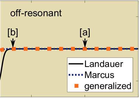
2
II. THEORY approximation.30,41 We will assume that each of the leads
has a constant density of states [̺l (ǫ) = const. where
We are interested in molecular junctions comprising a l = L, R] and that the electronic coupling between the
molecular system weakly coupled to two metallic elec- molecular energy level and a continuum of energy levels
trodes. At zero bias the molecular system within the in the leads is also constant (Vl = const. where Vl is the
junction is found in the N charge state. As the bias is molecule-lead coupling matrix element).
increased, the charging of the molecule – populating the The populations of the N (PN ) and N + 1 (PN +1 )
N + 1 (or N − 1) charge state – will eventually become charge states can be found by considering the following
possible. For simplicity, we assume that each of the two pair of rate equations:
considered charge states is non-degenerate, and ignore
any excited electronic states. Then, the molecular sys- dPN
= −(kL + kR )PN + (k̄L + k̄R )PN +1 , (1)
tem in question can be modelled as a single energy level dt
with energy ε0 which corresponds to the chemical poten- dPN +1
= −(k̄L + k̄R )PN +1 + (kL + kR )PN , (2)
tial for the charging of the molecular system. We note dt
that, generally, in the presence of electron-vibrational in-
teractions and molecule-lead coupling, the position of the where kl and k̄l are the rates of electron hopping on and
molecular energy level will be renormalized as compared off the molecular structure at the l interface, respectively,
to its gas-phase value. Since, experimentally, the position as denoted in Fig. 1. In the steady-state limit, dPN /dt =
of the molecular level is typically an empirical parameter, dPN +1 /dt = 0, it has the solution
here we simply absorb all these renormalizations into ε0 .
k̄L + k̄R
PN = , (3)
(a) kL + kR + k̄L + k̄R
kL kR
and PN +1 = 1 − PN . The current through the junc-
tion can be determined by considering either the left or
the right molecule-lead interface. Considering, for in-
stance, the left interface, the current through the junc-
tion is given by:
kL kR
I = e kL PN − k̄L PN +1 , (4)
(b) which gives the well-known expression:29,30
K+()
kL k̄R − kR k̄L
I=e . (5)
0 kL + kR + k̄L + k̄R
L
R Although in this work we shall consider a non-degenerate
electronic level, the (spin) degeneracy of the electronic
level in question can be relatively easily introduced into
fL() fR( ) this model, see for instance Ref.24 .
K-() The rates of electron transfers in Eq. (5) are given
by:34,42,43
Z ∞
2 dǫ
kl = Γl fl (ǫ)K+ (ǫ) , (6)
~ −∞ 2π
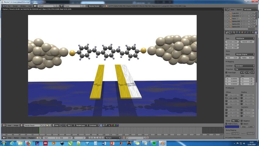
FIG. 1. (a) Artistic impression of a single-molecule junction. Z ∞
The effective rates of electron transfer on and off the molecular 2 dǫ
k̄l = Γl [1 − fl (ǫ)]K− (ǫ) , (7)
system are denoted by kL , kR and k̄L , k̄R , respectively. (b) ~ −∞ 2π
Schematic illustration of the rate-equation model considered
here; fl (ǫ) denotes the Fermi distribution in the lead l. K± (ǫ) where fl (ǫ) = 1/[exp((ǫ − µl )/kB T ) + 1] is the Fermi
are the molecular densities of states. distribution, µl is the chemical potential of the lead l,
and Γl is the strength of the molecule-lead interaction:
In this work it will be sufficient to model charge trans-
port through the junction using a rate equation ap- Γl = 2π|Vl |2 ̺l , (8)
proach. As schematically shown in Fig. 1, charge trans-
port through the weakly-coupled single-molecule junc- where ̺l is the (constant) density of states in the lead l
tion can be modelled as a series of electron transfers (we make use of this wide-band approximation through-
taking place at the left (L) and right (R) electrode. out). K± (ǫ) are the molecular densities of states for the
In what follows, we will work within the wide-band relevant processes. As we shall demonstrate in Section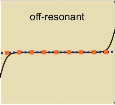
3

II A, they are given by                                          as it is done within the Marcus theory49 (although a num-
            Z ∞                                                  ber of ways to include nuclear tunnelling in a Marcus-
                          1                                      type description have been developed34,50,51 ). Later, we
   K± (ǫ) =       dE √         ×
              −∞       4πλk BT                                   will also assume that the nuclear degrees of freedom are
          [λ ± (E − T ∆S ◦ − ǫ)]2                                thermalized at all times. [We note that methods ac-

                                          Γ
  exp −                                             , (9)        counting for non-equilibrium vibrational effects in charge
                   4λkB T           (E − ε0 )2 + Γ2
                                                                 transfer and transport (while treating the vibrational en-
where λ is the classical reorganisation energy, Γ is the life-   vironment classically) have also been developed.52–54 ] In
time broadening, Γ = (ΓL + ΓR )/2, and ∆S ◦ the entropy          the classical limit, FWCD is therefore given by:37,39,47,48
change associated with the considered heterogeneous
electron transfer (∆S ◦ typically takes negative values                                           [λ + (∆E − T ∆S ◦ )]2

                                                                                   1
when charged species are produced in a polar solvent).             FCWD = √               exp −                             ,
                                                                                 4πλkB T                   4λkB T
The entropic effects, which will be discussed below, arise                                                                (11)
from the presence of the T ∆S ◦ term in Eq. (9) and,             where λ is the reorganisation energy, and ∆E and ∆S ◦
physically, stem predominantly from the changes in the           are the energy and entropy differences between the ‘prod-
solvent librational-rotational frequencies of the solvent        ucts’ and the ‘reactants’ of the considered process, re-
which depend on the charge on the electroactive molecule         spectively.
in the junction (an effect omitted in all ‘spin-boson’ treat-       Here, we wish to account for the fact that due to the
ments of electron transfer).37 We note that the entropic         coupling to metallic leads, the state corresponding to the
effects are therefore not accounted for in descriptions of       ‘products’ has a finite lifetime (i.e. is lifetime-broadened,
molecular conduction which treat the nuclear environ-            see Fig. 2). We therefore assume that the electronic state
ment quantum-mechanically. It is well-known however              corresponding to the ‘products’ comprises a continuum
that they can play a significant role in electron transfer       of states with the molecular density of states ρ(E) such
reactions in polar solvent environments.37,44,45                 that:
   What is the physical meaning of the Eqs. (6) and (7)?                              Z ∞
The overall rate of electron transfer from the lead onto
                                                                                           dE ρ(E) = 1 .                  (12)
the molecule (kl ) can be understood as a sum of the rates                            −∞
for all the possible electron transfers from the continuum
of donor states (the population of each of which is deter-          Then, the rate of electron transfer (between the single
mined by the Fermi-Dirac distribution), and conversely           considered metallic band and the molecular energy level)
for the rate of an electron transfer off the molecular sys-      is given by the integral:
tem (k̄l ). Γl in Eq. (8), in units of ~, is the well-known                  Z ∞
Golden Rule rate constant for electron transfer from the                ET             2π
                                                                       k =         dE      |Vl |2 FCWD(E) ρ(E) ,       (13)
electronic state of the molecule into the electronic states                    −∞       ~
of the lead, evaluated at the same energy. By microscopic
reversibility the rate constant for the isoenergetic reverse     where the FCWD(E) is given by:
step has the same value.
                                                                                                 [λ + (E − T ∆S ◦ − ǫ)]2

                                                                                    1
                                                                 FCWD(E) = √               exp −                           .
                                                                                 4πλkB T                 4λkB T
A.   Expression for the rate constant                                                                                (14)
                                                                   In order to determine ρ(E), let us consider the wave-
   In this section, we provide an intuitive derivation for       function ψ(t) for the molecular energy level. It can be
the molecular densities of states K± (ǫ) from the perspec-       written (in units of ~) as:
tive of the classical theory of electron transfer. For more
rigorous derivation we refer the reader to our earlier work            ψ(t) = θ(t) [exp(−iε0 t)] [exp(−Γt)] ψ(0) ,       (15)
in Ref. 34 (leading, however, to the omission of the en-
tropic term in Eq. (9)).                                         where θ(t) is the Heaviside step function, Γ/~ is the life-
   Let us consider a (non-adiabatic) electron transfer be-       time (decay constant) for the state in question, and we
tween a single band in a metallic lead l (with electro-          assume that ψ(0) is normalized. In the energy space, the
chemical potential ǫ) and the molecular level in question        corresponding function can be obtained by means of a
(with energy ε0 ). According to the conventional theory          Fourier transform:
of non-adiabatic electron transfer, the rate constant of                  Z ∞
this process is given by39,46–48                                  φ(E) =        dt ψ(t) exp(iEt) = ψ(0)/(Γ + i(E − ε0 )) .
                                                                            −∞
                         2π
                 k ET =     |Vl |2 FCWD ,            (10)                                                            (16)
                          ~                                      The probability density ρ(E) is proportional to |φ(E)|2 ,
where Vl is the coupling matrix element and FCWD is the          i.e.
Franck-Condon-weighted density of states. In what fol-
lows, we shall treat the vibrational dynamics classically                           ρ(E) = C 2 |φ(E)|2 ,                 (17)
4
Gaussian function becomes
E
[λ ± (E − T ∆S ◦ − ǫ)]2
1
√ exp − → δ(E − ǫ) ,
EM - 4πλkB T 4λkB T
(20)
EM + ‡ and Eq. (9) simplifies to
Γ
K± (ǫ) = , (21)
nuclear configuration (ǫ − ε0 )2 + Γ2
FIG. 2. Schematic illustration of the origins of the generalized where the molecular densities of states are identical for
theory. Parabolas describe the free energies of the reactants an electron transfer on and off the molecular system (mi-
and products (of the considered electron transfer) as a func- croscopic reversibility). Inserting Eq. (21) into Eq. (5)
tion of the nuclear coordinate. Molecule-lead coupling results allows us to reduce the expression for electric current to
in broadening of the parabola corresponding to the N + 1 the usual Landauer (Landauer-Büttiker) approach.55–59
charge state (M− ). Note that the shading does not show the It becomes:
dramatic effect that the Lorentzian tails can have on K± (ǫ).
e ∞ dǫ
Z
I= (fL (ǫ) − fR (ǫ)) T (ǫ) , (22)
~ −∞ 2π
where C is the normalisation factor. Since |ψ(0)|2 = 1,
we obtain where T (ǫ) is the transmission function, here given by a
Breit-Wigner resonance:60
Γ
ρ(E) = . (18)
π[(E − ε0 )2 + Γ2 ] ΓL ΓR
T (ǫ) = . (23)
(ǫ − ε0 )2 + Γ2
The electron-transfer rate given in Eq. (13) therefore
becomes Furthermore, it is instructive to consider the Landauer
Z ∞ approach in the limit of zero temperature and for a con-
2π 1 stant transmission function T (ǫ) = T . Then, Eq. (22)
k ET = dE |Vl |2 √ ×
−∞ ~ 4πλkB T becomes:
[λ + (E − T ∆S ◦ − ǫ)]2
Γ e e2
exp − . I= (µL − µR )T = Vb T . (24)
4λkB T π[(E − ε0 )2 + Γ2 ] h h
(19)
Introducing an additional factor of two to account for
The overall (effective) rate of electron transfer from the the spin degeneracy of the considered level, we recover
metallic electrode and onto the molecular level (or vice the celebrated Landauer formula for the electronic con-
versa) is simply a sum of the rates of individual electron ductance:
transfers weighted by the Fermi distribution and the lead
dI 2e2
density of states, as described by Eqs. (6) and (7). From G= = T , (25)
Eq. (19) we therefore obtain the expression for K± (ǫ) dVb h
given in Eq. (9). This result constitutes the basis of what
where T can vary between 0 and 1.55,61 For complete-
we will refer to as a generalized theory (which shall be
ness, an alternative derivation of Eq. (25) is given in the
discussed in greater detail in Section II C).
Appendix A.
Next,
√ we consider Eq. (9) in the limit when
Γ/ 4λkB T → 0, that is when the width of the Lorentzian
B. Landauer and Marcus limits
profile is negligible compared to that of the Gaussian pro-
file. Then,
In this section we will demonstrate that the conven-
tional Landauer and Marcus theories can be obtained as Γ
→ π δ(E − ε0 ) , (26)
the limiting cases of the generalized theory. As can be (E − ε0 )2 + Γ2
seen in Eq. (9), K± (ǫ) in the generalized theory is given
by a convolution of the Lorentzian and Gaussian profiles. and K± (ǫ) in Eq. (9) take the familiar form:
Let us first consider
√ the case of vanishing reorganisation
[λ ± (ε0 − T ∆S ◦ − ǫ)]2
r
energy. Then, 4λkB T /Γ → 0, i.e. the Gaussian pro- π
K± (ǫ) = exp − .
file in Eq. (9) becomes very narrow as compared to the 4λkB T 4λkB T
Lorentzian. We also know that with vanishing reorgani- (27)
zation energy the −T ∆S ◦ term also vanishes since the Together with Eqs. (6) and (7), Eq. (27) consti-
time is too short for the changes in polar solvent configu- tutes Marcus (Marcus-Levich-Dogonadze-Hush-Chidsey-
rations to contribute. In this limit, therefore, the relevant Gerischer) theory of transport.30,37,42,49,62,635
As was previously discussed,63 Landauer and Marcus
20
theories describe the opposite limits of charge transport K±( -ε0)
mechanism. The former describes transport as a coherent
K (eV-1)
process. In the latter, meanwhile, it is assumed that
before and following an electron transfer (from one of 10
K-( -ε0) K+( -ε0)
the metallic leads) the vibrational environment relaxes
and the charge density localizes on the molecular system
(until it tunnels out into the metallic lead).64
0
-1 -0.5 0 0.5 1
C. Back to the generalized approach - ε0 (eV)
Here, we return to the generalized theory derived in
Section II A which, as we have shown above, unifies the
conventional Marcus and Landauer theories of molecular FIG. 3. Molecular densities of states K± (ǫ) as present in the
conduction. (We note that the performance of our gen- (i) Landauer approach [solid thick line], (ii) Marcus theory
eralized theory is yet to be validated in the intermediate [solid lines], and (iii) generalized theory [dashed lines]. K± (ǫ)
were calculated for instructive values of λ = 0.3 eV and Γ = 50
regime, between the Landauer and Marcus limits, by a
meV at T = 300 K. For simplicity, we also set ∆S ◦ = 0.
detailed comparison with exact quantum-mechanical cal-
culation or experiment.) As can be clearly seen in Eq. (9),
the molecular densities of states K± (ǫ) in the generalized
theory are given by a Voigt function (a convolution of a this approach in various transport regimes, and compare
Gaussian and a Lorentzian).65 it to that predicted by the conventional Landauer and
It is instructive to consider Eq. (9) far away from res- Marcus approaches.
onance, i.e. when |ǫ − ε0 | ≫ λ, kB T, Γ. In this limit, the
Lorentzian and Gaussian profiles in Eq. (9) are centered
very far apart from each other (on the E-axis) so that the D. Some general remarks
wings of the Lorentzian are virtually constant over the
width of the Gaussian profile. Consequently, the inte-
gral in Eq. (9) returns simply the value of the Lorentzian In summary, charge transport through a weakly-
profile (far away from the resonance). Therefore, as we coupled molecular junction (modelled as a single elec-
also more rigorously show in Appendix B, far away from tronic level) can be described as a series of electron trans-
resonance the K± (ǫ) in Eq. (9) can be approximated as: fers with the molecular densities of states taking a form
of a Lorentzian (Landauer approach), Gaussian (Marcus
Γ theory), and Voigt functions (generalized theory), as in
K± (ǫ) ≈ . (28)
(ǫ − ε0 )2 Fig. 3. We note that within all of these approaches71
This is a significant result for several reasons. Firstly, we Z ∞
dǫ
note that far from resonance K± (ǫ) are independent of 2 K± (ǫ) = 1 , (29)
temperature. Furthermore, in the limit of |ǫ − ε0 | ≫ Γ, −∞ 2π
the same expression can be obtained from the Landauer
expression for K± (ǫ) given in Eq. (21). Therefore, the so that at very high bias kL = ΓL /~, k̄R = ΓR /~, and
generalized theory coincides with the Landauer approach kR = k̄L = 0, or vice versa. Therefore, in the limit of
not only for vanishing reorganisation energy (as we have very high bias voltage, we obtain the well-known value
previously discussed) but also far away from resonance: of electric current:
in the deep off-resonant regime an interacting system can
be approximated as a non-interacting one. This result e ΓL ΓR
I= , (30)
is in agreement with a multitude of experimental stud- ~ ΓL + ΓR
ies which, as discussed above, successfully modelled off-
resonant transport using the Landauer approach. Off- which is independent of the chosen theoretical approach
resonant charge transport is often the mechanism of con- (and so also of the strength of the vibrational coupling).
duction through molecular junctions especially at rela- We again stress that all the theories discussed here as-
tively low bias voltage and it is possible that it may also sume the presence of only a single molecular electronic
account for the long-range electron transport observed energy level (in each of the two considered charge states).
through DNA-based systems.66–69 They are therefore valid (in their presented form) at suf-
In our previous work, we have studied the IV char- ficiently low bias voltages such that the excited electronic
acteristics and the thermoelectric response predicted by states can be disregarded, and far away from the remain-
the generalized theory.34,70 Here, we will explore the ing charge degeneracy points (where populating charge
temperature-dependence of electric current predicted by states other than N and N + 1 becomes possible).6
E. Single-barrier model lower values of current as the molecular energy level en-
ters the bias window. This is fundamentally an exam-
In the above, the molecular system within the junc- ple of a Franck-Condon blockade.80,81 Furthermore, due
tion was effectively modelled as a well potential with two to relatively small Γ, the Marcus and generalized the-
tunnelling barriers – one at each of the molecule-lead in- ory predict seemingly very similar behavior. As we shall
terfaces. It is also worth to mention another relatively demonstrate (vide infra), the differences between these
simple theoretical model which is somewhat complemen- approaches become appreciable in the off-resonant trans-
tary to what has been discussed here. Namely, it is port regime.
possible to approximately model the molecular junction
as a single (typically trapezoidal) tunnelling barrier,72–75 (a) α = 0.5
and obtain the current-voltage characteristics using the 10 -7
Simmons model.76 Within this approach, no additional
1 resonant
charge density can localise on the molecule. It does not
Current (A)
therefore account for the reorganisation of the vibrational
environment associated with the charging of the molecule 0
in the junction and is typically justified only in a deep
off-resonant regime. This approach has been success- -1
fully used to account for the observed charged transport
through molecular system with high-lying molecular en- -2 -1 0 1 2
ergy levels.72–75 Bias Voltage (V)
(b) α = 0.9
III. COMPARISON OF THE CONDUCTION THEORIES -7
10
In this section, we explore the temperature-dependence Current (A) 1 resonant
of the electric current as predicted by the three ap-
proaches described above. We first calculate the IV char- 0 [c]
acteristics for the energy level lying at ε0 = 0.5 eV above
the Fermi levels of the unbiased leads. Where appropri- [d]
ate, we set λ = 0.3 eV (c.f. Ref.24 ), assume relatively -1
weak and symmetric molecule-lead coupling: ΓL = ΓR =
-2 -1 0 1 2
1 meV and, for simplicity, set T ∆S ◦ = 0. Experimen-
Bias Voltage (V)
tally, values of lifetime broadening from less than 1 µeV
up to a few hundred meV have been observed.24,25,77,78
FIG. 4. IV characteristics calculated using the Landauer,
This large spread in the observed Γ stems most likely Marcus and generalized approaches for: (a) α = 0.5, and (b)
from variations in the nature of molecule-lead contacts α = 0.9. We set the position of the molecular level above the
(the electronic coupling is typically assumed to decay ex- Fermi level of the unbiased leads ε0 = 0.5 eV, ΓL = ΓR = 1
ponentially with distance) as well as in the densities of meV, λ = 0.3 eV (in Marcus and generalized approaches), and
states in the metallic electrodes (which depend on the ex- T = 300 K. The shaded area marks the off-resonant regime
act atomic structure of the metallic tips). The chemical (when the molecular level lies outside of the bias window).
potentials of the leads are determined by the applied bias Note that Marcus and generalized theory curves appear to
voltage Vb : µL = −|e|αVb and µR = |e|(1−α)Vb . The pa- closely overlap in the resonant transport regime.
rameter α accounts for how the potential difference is dis-
tributed between the left and right electrodes (and varies We now turn to examine the temperature dependence
between 0 and 1), see Ref.79 for a detailed discussion. In of the electric current as predicted by the three ap-
particular if α = 0.5, the bias voltage is applied symmet- proaches considered here. This is done in Fig. 5 which
rically resulting in a symmetric IV curve. Otherwise, shows the electric current as a function of temperature
the bias is applied asymmetrically giving rise to current (on an Arrhenius plot) for different values of the bias volt-
rectification (asymmetrical IV characteristics).17,78 age. We consider current at four different bias voltages
We begin by calculating the IV characteristics for [as marked by arrows in Fig. 4(b)], initially disregarding
α = 0.5 and α = 0.9 in Fig. 4(a) and (b), respectively. the entropic effects (∆S o = 0).
All of them exhibit the expected behavior (for a single- Within the Landauer approach, the temperature de-
level model): region of suppressed current at low bias pendence of the electric current stems solely from the
voltage (where the molecular energy level is found out- temperature dependence of the Fermi distributions in the
side of the bias window) followed by a rise in current and leads. Consequently, the electric current is almost inde-
an eventual plateau in the deep resonant regime. In the pendent of temperature when the molecular energy level
presence of electron-vibrational interactions (i.e. within lies far away from the bias window [Fig. 5(a)], increases
the Marcus and generalized approaches), we can observe with temperature in the case of near-resonant transport7
(a) Vb = +1 V (b) b = -0.4 V
-3 -2.5
-4
ε0 0 -3
-5
μL
μR
ln|I( A)|
A)|
-3.5
-6 μR
logln|I(
-7
10
-4
log10
μL
-8
Landauer Landauer
-4.5
-9 Marcus Marcus
generalized generalized
-10 -5
3 3.5 4 3 3.5 4
-3
1/T (K-1) 10 1/T (K-1) 10 -3
(c) b = -0.8 V (d) b = -1.2 V
-0.8 μL -0.9
μL λ -0.9
0 λ
0 -0.91
-1
A)|
A)|
-1.1 μR
μR -0.92
logln|I(
logln|I(
-1.2
10
10
-1.3
Landauer -0.93 Landauer
-1.4 Marcus Marcus
generalized generalized
-1.5 -0.94
3 3.5 4 3 3.5 4
1/T (K-1) 10 -3 1/T (K-1) 10 -3
FIG. 5. Arrhenius plots of electric current [log 10 (I) vs. 1/T ] at bias voltage Vb = {1, −0.4, −0.8, −1.2} V as a function of
temperature. Other parameters as in Fig. 4(b): α = 0.9, ΓL = ΓR = 1 meV, λ = 0.3 eV. Left panels schematically show the
relative positions of the molecular energy level and the chemical potentials of the leads (for clarity, broadening of the Fermi
distributions in the leads is not shown).
[Fig. 5(b)], and decreases with increasing temperature states K± (ǫ) leads to a modest decrease in current with
in the resonant transport regime [Figs. 5(c) and (d)] al- increasing temperature [Fig. 5(d)].
though this effect can be relatively modest. Finally, we consider the generalized theory. Within
In contrast, within the Marcus approach, the this approach, the temperature dependence of electric
temperature-dependence is determined by both the tem- current once again stems from the broadening of the
perature dependence of the Fermi distributions in the Fermi distributions as well as temperature dependence
leads and that of the Marcus rates in Eq. (27). The of the electron transfer rates. The temperature depen-
latter contribution typically dominates and usually ex- dence of K± (ǫ) given in Eq. (9) is, however, rather non-
hibits an exponential dependence on inverse tempera- trivial. In the deep off-resonant regime [Fig. 5(a)], elec-
ture. Indeed, we observe an Arrhenius-type behavior tric current is virtually independent of temperature and
in the far off-resonant scenario [Fig. 5(a)]: electric cur- takes values similar to those predicted by the Landauer
rent depends exponentially on inverse temperature and is approach, see discussion in Section II C. In the near-
greatly suppressed, as compared to that predicted by the resonant case [Fig. 5(b)], electric current generally in-
Landauer theory. The same is true in the near-resonant creases with increasing temperature although in a non-
case [Fig. 5(b)]. In the resonant regime, the electric cur- linear fashion different from what is predicted by both the
rent increases (in an Arrhenius-type fashion) with tem- Landauer and Marcus transport theories. Conversely, in
perature as long as the chemical potential of the left lead the resonant regime the predictions of the generalized
satisfies µL < ε0 + λ [Fig. 5(c)].63 In the deep resonant theory closely coincide with those of the conventional
regime (for µL > ε0 + λ), broadening of both the Fermi Marcus theory.
distributions in the leads and the molecular densities of These results illustrate the fact that both the Lan-8
dauer and Marcus theories can be used to describe charge (a)
transport through molecular junctions in their respective
regimes of applicability. As discussed above, these differ-
ent regimes may even correspond to different ranges of T = 250 K,
bias voltage for the same molecular junction. T = 350 K,
T = 250 K,
T = 350 K,
IV. ENTROPIC EFFECTS
We next investigate the role of entropic effects
in molecular conduction. In accordance with previ- (b) Generalized theory (c) Marcus theory
ous experimental studies of electron transfer in polar
solvents,82–84 we set ∆S o = −40 J K−1 mol−1 (which
corresponds to roughly -0.41 meV K−1 ) unless stated oth-
erwise. First, in Fig. 6(a), using our generalized theory,
we calculate the IV characteristics obtained for ∆S o = 0
and −40 J K−1 mol−1 and at different temperatures. The
current steps, present in the IV characteristics when the
molecular energy level falls into the bias window, are sig-
nificantly shifted for non-zero ∆S o . Furthermore, in the
presence of entropic effects, the magnitudes of those shifts
are increasing with temperature, while for ∆S o = 0 in-
creasing temperature leads solely to the broadening of
the IV characteristics. In the resonant (high-current)
region, qualitatively identical behavior is also predicted
by the conventional Marcus theory (not shown). FIG. 6. (a) IV characteristics calculated at different temper-
The origin of both of these effects can be under- atures for ∆S o = −40 and 0 J K−1 mol−1 . Other parameters
stood using Eq. (9): the inclusion of entropic effects as in Fig. 5. (b, c) Temperature dependence of the electric
corresponds to an effective (and temperature-dependent) current at Vb = +0.5 V calculated using the (b) generalized
renormalization of the position of the molecular energy and (c) conventional Marcus theory.
level. For negative ∆S o , this results in a shift of the
current step toward higher values of bias voltage (shift
in the opposite direction will be observed in the case of
transport through a level found below the Fermi level
of the unbiased leads). From Eqs. (9) and (27), it can
be inferred that strong entropic effects should be ex- teractions). In the presence of negative ∆S o , we observe
pected when λ + (ε0 − ǫ) = 0. It can be indeed seen lower values of electric current through the junction (once
in Fig. 6(a) that inclusion of negative ∆S o leads to a again due to the temperature-dependent shift of the effec-
negative temperature coefficient of the current (decreas- tive position of the molecular level). The electric current
ing current with increasing temperature) in the resonant predicted by the generalized theory [Fig. 6(b)] exhibits
regime. Analogous negative temperature coefficient has only fairly weak temperature dependence, in accordance
been seen experimentally in charge recombination elec- with previous discussion. In the case of non-zero ∆S o ,
tron transfer reactions in polar liquids when the intrinsic the current very unusually decreases with increasing T
barrier to reaction is small and has been discussed in as the temperature dependence is dominated by the en-
the literature.37,45 The decrease of electric current with tropic effect. This can again be explained by the effective
increasing temperature can occur when ∆S o is negative renormalization of the position of the molecular level by
and the molecular energy level is found above the Fermi the entropic term. On the other hand, within the conven-
levels of the unbiased leads or when ∆S o is positive and tional Marcus theory [Fig. 6(c)], we once again observe
the and the molecular energy level is found below the Arrhenius-type characteristics. Unlike the magnitude of
Fermi levels of the electrodes. We also note that the the current, its temperature-dependent behavior is not
qualitative behavior of the electric current in the reso- significantly affected by the entropic effects.
nant regime (as a function of temperature) could be used
to experimentally determine the sign of ∆S o . In summary, entropic effects (of a realistic magnitude)
In Figs. 6(b) and (c), we further consider the tem- can result in an unusual temperature-dependent behav-
perature dependence of the electric current in the off- ior of the electric current. Negative temperature coef-
resonant regime using the generalized and conventional ficient in particular may serve as an indication of this
Marcus theory, respectively (we do not consider here the phenomenon in experimental studies on solvated molec-
Landauer theory since it disregards the environmental in- ular junctions.9
V. MARCUS-LEVICH-DOGONADZE-JORTNER 8
DESCRIPTION gMLDJ
6 generalized
K (eV-1)
Thus far, the entire vibrational environment was 4
treated classically. It is well-known, however, that K-( -ε0) K+( -ε0)
2
the high-temperature assumption of Marcus theory is
generally not valid at around room temperature for 0
the high-frequency molecular modes. These modes -2 -1 0 1 2
should be treated quantum-mechanically in order to (eV)
obtain a qualitative agreement with the experimental
studies.85,86 This need motivated Jortner and cowork- FIG. 7. Molecular densities of states K± (ǫ) calculated for
ers to develop an extension of the classical Marcus Γ = 5 meV, λout = 150 meV, D = 1.9, ω0 = 190 meV
theory, known as the Marcus-Levich-Dogonadze-Jortner (gMLDJ), and λ = λout +Dω0 (generalized theory) at T = 300
theory.47,51 Within this approach, molecular vibrational K. For simplicity, ∆S ◦ = 0.
environment is divided into two components: the low-
frequency part typically associated with the outer-sphere
environment, and the high frequency part represented are given by:
by a single effective mode of frequency ω0 . This ef- ∞ Z ∞
Dm
r
fective high-frequency mode typically represents molec- π X
K± (ǫ) = e−D × dE
ular vibrational modes corresponding to carbon-carbon 4λout kB T m=0 m! −∞
and carbon-oxygen double-bond stretches (ubiquitous to
[(λout + mω0 ) ± (E − T ∆S ◦ − ǫ)]2
most organic structures) and has a frequency of roughly Γ
exp − × .
190 meV (∼ 1500 cm−1 ). Then, the rate of electron 4λout kB T (E − ε0 )2 + Γ2
transfer is given by Eq. (10) with the Franck-Condon- (33)
weighted density of states51
This constitutes what we shall refer to as the generalized
Marcus-Levich-Dogonadze-Jortner (gMLDJ) theory.
∞ In Fig. 7, we plot the molecular densities of states
1 X Dm K± (ǫ) obtained using the generalized Marcus and gener-
FCWD = √ e−D
4πλout kB T m=0 m! alized MLDJ approaches. The latter clearly shows a set
[∆E − T ∆S ◦ + λout + mω0 ]2
of equidistant peaks separated by ω0 which correspond to
exp − , (31) the excitations of the (effective) high-frequency molecular
4λout kB T
mode. Since this high-frequency vibrational mode con-
stitutes a somewhat phenomenological description of the
inner-sphere environment (which in reality comprises a
where λout is the outer-sphere reorganisation energy. D
set of vibrational modes), the presence of these equally-
is the Huang-Rhys parameter for the coupling to the ef-
spaced conductance peaks is an artefact of the Marcus-
fective high-frequency vibrational mode
Levich-Dogonadze-Jortner approach. Furthermore, the
Marcus-Levich-Dogonadze-Jortner approach predicts a
λin much larger magnitude of K± (ǫ) (as compared to the
D= , (32) classical Marcus rates) for both smaller and larger values
ω0 of |ǫ − ε0 |, a direct result of incorporating nuclear tun-
nelling in the Marcus-Levich-Dogonadze-Jortner theory.
All these aspects of Marcus-Levich-Dogonadze-Jortner
where λin is the corresponding reorganisation energy.
theory have long been well-understood.38 We note that
Marcus-Levich-Dogonadze-Jortner theory (in its original
nuclear tunneling is much more important in the inverted
formulation as well as its multi-mode extension) has be-
regime than in the normal regime.
come the most commonly used way to introduce nuclear
tunnelling into the description of electron transfer.38 We In an analogy to what was discussed in Section II B,
recall that in the conventional Levich-Dogonadze and all by setting λout = λin = 0 in the gMLDJ theory we again
similar quantum mechanical treatments the medium in recover the Landauer description of transport. Once
which the charges exist do not contain a ∆S o term be- again, lifetime broadening again becomes especially rel-
cause of the assumptions tacitly made in treating the evant in off-resonant regime of transport. Qualitatively,
environment quantum mechanically. the behavior which is predicted by this approach in the
off-resonant regime will coincide with that of the gen-
It is also possible to adapt this theory in the transport eralized theory: inclusion of lifetime broadening will
setting considered here and incorporate lifetime broaden- result in increased electric current and its very weak
ing into this framework. Using Eq. (13) and the FCWD temperature dependence, c.f. Section III. Finally, we
factor given in Eq. (31), the relevant densities of states note that lifetime broadening can also be introduced in10
the multi-mode extension of Marcus-Levich-Dogonadze- Appendix A: Alternative derivation of the Landauer formula
Jortner theory (where it would normally be necessary to
calculate the Huang-Rhys factor for each of the molecu-
lar modes).47,51 This modification would lead, however, To derive the Landauer formula for the electronic con-
to an even more complicated expression and we see lit- ductance, let us consider a one-dimensional wire connect-
tle advantage in using such an approach in practical ap- ing two electronic reservoirs with electrochemical poten-
plications (as opposed to, for instance, the generalized- tials µL and µR , respectively. If the length of the wire is
quantum-master-equation result of Ref. 34). given by L, then the electric current through the consid-
ered system is (at zero temperature) given by:
v
I = e n+ , (A1)
VI. CONCLUDING REMARKS L
where v is the velocity of the charge carriers within the
In this work, we first focused on the recently-derived wire and n+ is the number of states for electrons propa-
generalized theory. We have presented an intuitive gating from left to right within the bias window (i.e. be-
derivation of this approach, showed how entropic effects tween µL and µR ). Assuming that the wire possess a
can be incorporated into that formalism, and demon- (quasi-)continuum of states, we can write
strated how the conventional Landauer and Marcus ap-
proaches can be obtained as limiting cases of this more dn+ v
I = e (µL − µR ) . (A2)
general approach. We have further demonstrated that dµ L
(for relatively weak molecule-lead coupling) the predic-
Here, dn+ /dµ is the density of states in the wire for elec-
tions of the generalized theory coincide very well with
trons moving from left to right.
those of Landauer and Marcus theories in the off-resonant
Let us assume that the considered wire can be de-
and resonant regime, respectively. Consequently, we
scribed with a square-well potential, Then the energies
believe that the generalized theory correctly describes
of the electronic levels are:
transport properties of molecular junctions across the en-
tire experimentally-accessible domain (i.e. in both the n2 h2
E= , (A3)
resonant and off-resonant regime; provided the high- 8mL2
temperature assumption of Marcus theory is justified).
where m is the mass of the charge carrier. Then, the
We have also studied the influence and identified exper-
density of states becomes
imental signatures of entropic effects in the molecular
electronic conduction in different transport regimes. Fi- dn+ 1 2L −1
nally, in Section V, we have shown how lifetime broad- =2× × v , (A4)
dµ 2 h
ening can be introduced into Marcus-Levich-Dogonadze-
Jortner theory. The theory presented here can be also where the factor of 2 accounts for the spin of the elec-
extended beyond the single-level model and thus intro- trons, while the factor of 1/2 accounts for the fact that
duce lifetime-broadening effects into the rate-equation we are interested only in the states corresponding to elec-
descriptions30 of multi-level molecular junctions.87 Our trons propagating from left to right. Inserting Eq. (A4)
hope is that this work will inspire a wide use of the the- into Eq. (A2), the current is given by:
ory described here in experimental studies on molecular 2e 2e2
junctions as well as stimulate empirical exploration of I= (µL − µR ) = Vb , (A5)
entropic effects in these systems. h h
giving the conductance Landauer expression for the con-
ductance for a perfectly-transmitting channel:
ACKNOWLEDGMENTS 2e2
G= . (A6)
h
JKS thanks Hertford College, Oxford for financial If the transmission through the wire is less than 1, the
support, and L. MacGregor for carefully reading the conductance can be expressed using Eq. (25).
manuscript. RAM thanks the Office of the Naval Re-
search and the Army Research Office for their support of
this research. Appendix B: Generalized theory far away from resonance
First, we note that Eq. (9) can be equivalently written
DATA AVAILABILITY STATEMENT as:34
(Γ − iν± )2
r
π Γ − iν±
K± (ǫ) = Re exp erfc √ ,
The data that supports the findings of this study are 4λkB T 4λkB T 4λkB T
available within the article itself. (B1)11
where ν± = λ ∓ (ǫ − ε0 + T ∆S ◦ ), Γ is again the lifetime which inserting the definition of x becomes,
broadening, and erfc(x) denotes a complementary √ error
function. Let us consider here the limit of Γ ≪ 4λkB T Γ
K± (ǫ) ≈ 2 . (B11)
and define ν±
Finally, setting
p
x :=ν± / 4λkB T ; (B2)
p
y :=Γ/ 4λkB T . (B3) ν± = [λ ∓ (ǫ − ε0 + T ∆S ◦ )]2 ≈ (ǫ − ε0 )2 , (B12)
Then, the molecular densities of states can be written as gives Eq. (28) in the main body of this work.
r 1 M. A. Reed, C. Zhou, C. Muller, T. Burgin, and J. Tour, Science
π 278, 252 (1997).
K± (ǫ) = Re[w(x + iy)] , (B4)
4λkB T 2 H. Park, J. Park, A. K. Lim, E. H. Anderson, A. P. Alivisatos,
and P. L. McEuen, Nature 407, 57 (2000).
3 J. Park, A. N. Pasupathy, J. I. Goldsmith, C. Chang, Y. Yaish,
where w(x + iy) is the Faddeeva function [the real part
of which (up to a factor) is the Voigt function], J. R. Petta, M. Rinkoski, J. P. Sethna, H. D. Abruña, P. L.
McEuen, et al., Nature 417, 722 (2002).
4 W. Liang, M. P. Shores, M. Bockrath, J. R. Long, and H. Park,
w(x + iy) = exp[(y − ix)2 ] erfc[y − ix] . (B5) Nature 417, 725 (2002).
5 X. Cui, A. Primak, X. Zarate, J. Tomfohr, O. Sankey, A. Moore,
We can now take the limit y ≪ 1 where Eq. (B5) can T. Moore, D. Gust, G. Harris, and S. Lindsay, Science 294, 571
be approximated [by considering the Taylor expansion of (2001).
6 C. Kergueris, J.-P. Bourgoin, S. Palacin, D. Estève, C. Urbina,
w(x + iy) around y = 0] as:88
M. Magoga, and C. Joachim, Phys. Rev. B 59, 12505 (1999).
7 M. L. Perrin, E. Burzurı́, and H. S. van der Zant, Chem. Soc.
2 2y
w(x + iy) ≈ e−x (1 − 2ixy)[1 + erf(ix)] − √ , (B6) Rev. 44, 902 (2015).
π 8 P. Gehring, J. K. Sowa, J. Cremers, Q. Wu, H. Sadeghi, Y. Sheng,
J. H. Warner, C. J. Lambert, G. A. D. Briggs, and J. A. Mol,
where erf(x) denotes the error function. Substituting ACS Nano 11, 5325 (2017).
9 M. Elbing, R. Ochs, M. Koentopp, M. Fischer, C. von Hänisch,
Eq. (B6) to Eq. (B4) gives (after some rearrangements):
F. Weigend, F. Evers, H. B. Weber, and M. Mayor, Proc. Natl.
Acad. Sci. U.S.A. 102, 8815 (2005).
[λ ∓ (ǫ − ε0 + T ∆S ◦ )]2
r
π 10 I. Dı́ez-Pérez, J. Hihath, Y. Lee, L. Yu, L. Adamska, M. A.
K± (ǫ) ≈ exp − Kozhushner, I. I. Oleynik, and N. Tao, Nat. Chem. 1, 635 (2009).
4λkB T 4λkB T 11 M. L. Perrin, E. Galán, R. Eelkema, J. M. Thijssen, F. Grozema,
λ ∓ (ǫ − ε0 + T ∆S ◦ )
Γ and H. S. van der Zant, Nanoscale 8, 8919 (2016).
+ √ 12 C. Iacovita, M. Rastei, B. Heinrich, T. Brumme, J. Kortus,
λkB T 4λkB T
L. Limot, and J. Bucher, Phys. Rev. Lett. 101, 116602 (2008).
λ ∓ (ǫ − ε0 + T ∆S ◦ )
1 13 S. Sanvito, Chem. Soc. Rev. 40, 3336 (2011).
D √ − , (B7) 14 L. Bogani and W. Wernsdorfer, Nat. Mater. 7, 179 (2008).
4λkB T 2
15 P. Reddy, S.-Y. Jang, R. A. Segalman, and A. Majumdar, Sci-
where D(x) denotes a Dawson function. We note here ence 315, 1568 (2007).
16 L. Cui, R. Miao, C. Jiang, E. Meyhofer, and P. Reddy, J. Chem.
that the first term on the right-hand side of Eq. (B7) is Phys. 146, 092201 (2017).
simply the Marcus rate from Eq. (27), so that the cor- 17 X. Chen, M. Roemer, L. Yuan, W. Du, D. Thompson, E. del
rection to the conventional Marcus rate is proportional Barco, and C. A. Nijhuis, Nat. Nanotechnol. 12, 797 (2017).
18 A. Nitzan, Annu. Rev. Phys. Chem. 52, 681 (2001).
to Γ. Since Eq. (B1) was derived for the case of weak 19 V. B. Engelkes, J. M. Beebe, and C. D. Frisbie, J. Am. Chem.
molecule-lead coupling,34 the (mathematical) validity of
Soc. 126, 14287 (2004).
Eq. (B7) typically coincides with the (physical) validity 20 S. M. Lindsay and M. A. Ratner, Adv. Mater. 19, 23 (2007).
of the generalized Marcus theory. 21 C. Jin, M. Strange, T. Markussen, G. C. Solomon, and K. S.
Next, we consider Eq. (B7) in the limit of large |ǫ − ε0 |, Thygesen, J. Chem. Phys. 139, 184307 (2013).
22 D. Secker, S. Wagner, S. Ballmann, R. Härtle, M. Thoss, and
|ǫ − ε0 | ≫ λ, kB T, Γ, T ∆S ◦ . (B8) H. B. Weber, Phys. Rev. Lett. 106, 136807 (2011).
23 E. Burzurı́, J. O. Island, R. Dı́az-Torres, A. Fursina, A. González-
Campo, O. Roubeau, S. J. Teat, N. Aliaga-Alcalde, E. Ruiz, and
Firstly, we note that the first term on the right-hand H. S. J. van der Zant, ACS Nano 10, 2521 (2016).
side of Eq. (B7) vanishes. Secondly, using the definition 24 J. O. Thomas, B. Limburg, J. K. Sowa, K. Willick, J. Baugh,
of x from Eq. (B2), we note that for large x, the Dawson G. A. D. Briggs, E. M. Gauger, H. L. Anderson, and J. A. Mol,
function can be approximated as: Nat. Commun. 10, 1 (2019).
25 E.-D. Fung, D. Gelbwaser, J. Taylor, J. Low, J. Xia, I. Davy-
1 1 denko, L. M. Campos, S. Marder, U. Peskin, and L. Venkatara-
D(x) ≈ + . (B9) man, Nano Lett. 19, 2555 (2019).
2x 4x3 26 E. P. Friis, Y. I. Kharkats, A. M. Kuznetsov, and J. Ulstrup, J.
Phys. Chem. A 102, 7851 (1998).
Then, 27 A. M. Kuznetsov and J. Ulstrup, J. Phys. Chem. A 104, 11531
(2000).
Γ 1 1 1 28 A. M. Kuznetsov and J. Ulstrup, J. Chem. Phys. 116, 2149
K± (ǫ) ≈ x + − , (B10)
λkB T 2x 4x3 2 (2002).12
29 J. Zhang, A. M. Kuznetsov, I. G. Medvedev, Q. Chi, T. Albrecht, 63 A. Migliore, P. Schiff, and A. Nitzan, Phys. Chem. Chem. Phys.
P. S. Jensen, and J. Ulstrup, Chem. Rev. 108, 2737 (2008). 14, 13746 (2012).
30 A. Migliore and A. Nitzan, ACS Nano 5, 6669 (2011). 64 It is interesting to note that a Gaussian profile is sometimes in-
31 A. Migliore and A. Nitzan, J. Am. Chem. Soc. 135, 9420 (2013). troduced ad hoc into the Landauer framework in order to explain
32 L. Yuan, L. Wang, A. R. Garrigues, L. Jiang, H. V. Annadata, the experimentally-observed behavior.17 .
M. A. Antonana, E. Barco, and C. A. Nijhuis, Nat. Nanotechnol. 65 B. H. Armstrong, J. Quant. Spectrosc. Radiat. Transf. 7, 61
13, 322 (2018). (1967).
33 C. Jia, A. Migliore, N. Xin, S. Huang, J. Wang, Q. Yang, 66 D. N. Beratan, R. Naaman, and D. H. Waldeck, Current Opinion
S. Wang, H. Chen, D. Wang, B. Feng, et al., Science 352, 1443 in Electrochemistry 4, 175 (2017).
(2016). 67 H. Kim, M. Kilgour, and D. Segal, The Journal of Physical
34 J. K. Sowa, J. A. Mol, G. A. D. Briggs, and E. M. Gauger, J. Chemistry C 120, 23951 (2016).
Chem. Phys. 149, 154112 (2018). 68 E. Wierzbinski, R. Venkatramani, K. L. Davis, S. Bezer, J. Kong,
35 J. K. Sowa, N. Lambert, T. Seideman, and E. M. Gauger, J. Y. Xing, E. Borguet, C. Achim, D. N. Beratan, and D. H.
Chem. Phys. 152, 064103 (2020). Waldeck, ACS Nano 7, 5391 (2013).
36 J. Liu and D. Segal, Phys. Rev. B 101, 155407 (2020). 69 P. Dauphin-Ducharme, N. Arroyo-Currás, and K. W. Plaxco, J.
37 R. A. Marcus and N. Sutin, Biochim. Biophys. Acta 811, 265 Am. Chem. Soc. 141, 1304 (2019).
(1985). 70 J. K. Sowa, J. A. Mol, and E. M. Gauger, J. Phys. Chem. C
38 P. F. Barbara, T. J. Meyer, and M. A. Ratner, J. Phys. Chem. 123, 4103 (2019).
100, 13148 (1996). 71 Naturally, this does not hold for the approximation of K (ǫ)
±
39 V. May and O. Kühn, Charge and energy transfer dynamics in
given in Eq. (28) which is valid only on the part of the energy
molecular systems (John Wiley & Sons, 2008). domain.
40 H. Kang, G. D. Kong, S. E. Byeon, S. Yang, J. W. Kim, and 72 S. H. Choi, B. Kim, and C. D. Frisbie, Science 320, 1482 (2008).
H. J. Yoon, J. Phys. Chem. Lett. 11, 8597 (2020). 73 J. M. Beebe, B. Kim, J. W. Gadzuk, C. D. Frisbie, and J. G.
41 M. Galperin, A. Nitzan, and M. A. Ratner, Phys. Rev. B 73,
Kushmerick, Phys. Rev. Lett. 97, 026801 (2006).
045314 (2006). 74 W. Wang, T. Lee, and M. A. Reed, Phys. Rev. B 68, 035416
42 C. E. Chidsey, Science 251, 919 (1991).
(2003).
43 H. Gerischer, Surf. Sci. 18, 97 (1969). 75 D. J. Wold and C. D. Frisbie, J. Am. Chem. Soc. 123, 5549
44 R. Marcus and N. Sutin, Comments Inorg. Chem. 5, 119 (1986).
(2001).
45 R. A. Marcus and N. Sutin, Inorg. Chem. 14, 213 (1975). 76 J. G. Simmons, J. Appl. Phys. 34, 1793 (1963).
46 R. P. Van Duyne and S. F. Fischer, Chem. Phys. 5, 183 (1974). 77 R. Frisenda and H. S. J. van der Zant, Phys. Rev. Lett. 117,
47 J. Ulstrup and J. Jortner, J. Chem. Phys. 63, 4358 (1975).
126804 (2016).
48 N. R. Kestner, J. Logan, and J. Jortner, J. Phys. Chem. 78, 78 B. Capozzi, J. Xia, O. Adak, E. J. Dell, Z.-F. Liu, J. C. Tay-
2148 (1974). lor, J. B. Neaton, L. M. Campos, and L. Venkataraman, Nat.
49 R. A. Marcus, J. Chem. Phys. 24, 966 (1956).
Nanotechnol. 10, 522 (2015).
50 J. J. Hopfield, Proc. Natl. Acad. Sci. U.S.A. 71, 3640 (1974). 79 S. Datta, W. Tian, S. Hong, R. Reifenberger, J. I. Henderson,
51 J. Jortner, J. Chem. Phys. 64, 4860 (1976).
and C. P. Kubiak, Phys. Rev. Lett. 79, 2530 (1997).
52 H. Sumi and R. Marcus, J. Chem. Phys. 84, 4894 (1986). 80 J. Koch and F. von Oppen, Phys. Rev. Lett. 94, 206804 (2005).
53 W. Dou, C. Schinabeck, M. Thoss, and J. E. Subotnik, J. Chem. 81 K. H. Bevan, A. Roy-Gobeil, Y. Miyahara, and P. Grutter, J.
Phys. 148, 102317 (2018). Chem. Phys. 149, 104109 (2018).
54 H. Kirchberg, M. Thorwart, and A. Nitzan, J. Phys. Chem. Lett. 82 G. Marrosu, F. Rodante, A. Trazza, and L. Greci, Thermochim-
11, 1729 (2020). ica acta 168, 59 (1990).
55 R. Landauer, IBM J. Res. Dev. 1, 223 (1957). 83 K. Komaguchi, Y. Hatsusegawa, A. Kitani, and K. Sasaki, Bull.
56 Y. Imry and R. Landauer, Rev. Mod. Phys. 71, S306 (1999).
Chem. Soc. Jpn. 64, 2686 (1991).
57 N. A. Zimbovskaya, Transport properties of molecular junctions, 84 M. Svaan and V. D. Parker, Acta Chem. Scand. B 38, 759 (1984).
Vol. 254 (Springer, 2013). 85 J. R. Miller, J. V. Beitz, and R. K. Huddleston, J. Am. Chem.
58 A. Nitzan, Chemical dynamics in condensed phases: relaxation,
Soc. 106, 5057 (1984).
transfer and reactions in condensed molecular systems (Oxford 86 G. L. Closs, L. T. Calcaterra, N. J. Green, K. W. Penfield, and
University Press, 2006). J. R. Miller, J. Phys. Chem. 90, 3673 (1986).
59 M. Esposito and M. Galperin, Phys. Rev. B 79, 205303 (2009). 87 However, an ad hoc replacement of the molecule-lead hopping
60 G. Breit and E. Wigner, Phys. Rev. 49, 519 (1936).
rates (in the conventional rate equation or quantum master equa-
61 R. Landauer, J. Phys.: Condens. Matter 1, 8099 (1989).
tion approaches) with the expressions developed here will yield a
62 S. Gosavi and R. A. Marcus, J. Phys. Chem. B 104, 2067 (2000).
theory that does not recover the exact Landauer result for molec-
ular systems with more than one site.
88 S. M. Abrarov and B. M. Quine, J. Math. Res. 7, 44 (2015).You can also read