Parametrization of a lake water dynamics model MLake in the ISBA-CTRIP land surface system (SURFEX v8.1) - GMD
←
→
Page content transcription
If your browser does not render page correctly, please read the page content below
Geosci. Model Dev., 14, 1309–1344, 2021
https://doi.org/10.5194/gmd-14-1309-2021
© Author(s) 2021. This work is distributed under
the Creative Commons Attribution 4.0 License.
Parametrization of a lake water dynamics model MLake in the
ISBA-CTRIP land surface system (SURFEX v8.1)
Thibault Guinaldo1 , Simon Munier1 , Patrick Le Moigne1 , Aaron Boone1 , Bertrand Decharme1 , Margarita Choulga2 ,
and Delphine J. Leroux1
1 Centre National de Recherches Météorologiques, Université de Toulouse, Météo-France, CNRS, Toulouse, France
2 Research Department, European Centre for Medium-Range Weather Forecasts (ECMWF), Reading, RG2 9AX, UK
Correspondence: Thibault Guinaldo (thibault.guinaldo@meteo.fr)
Received: 4 September 2020 – Discussion started: 10 November 2020
Revised: 28 January 2021 – Accepted: 1 February 2021 – Published: 10 March 2021
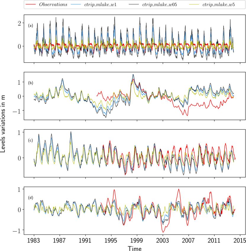
Abstract. Lakes are of fundamental importance in the Earth sensitivity to the width of the lake outlet. Regarding lake
system as they support essential environmental and eco- level variations, results indicate a good agreement between
nomic services, such as freshwater supply. Streamflow vari- observations and simulations with a mean correlation of 0.56
ability and temporal evolution are impacted by the presence (ranging from 0.07 to 0.92) which is linked to the capabil-
of lakes in the river network; therefore, any change in the ity of the model to retrieve seasonal variations. Discrepan-
lake state can induce a modification of the regional hydro- cies in the results are mainly explained by the anthropiza-
logical regime. Despite the importance of the impact of lakes tion of the selected lakes, which introduces high-frequency
on hydrological fluxes and the water balance, a representa- variations in both streamflows and lake levels that degraded
tion of the mass budget is generally not included in climate the scores. Anthropization effects are prevalent in most of
models and global-scale hydrological modeling platforms. the lakes studied, but they are predominant for Lake Victo-
The goal of this study is to introduce a new lake mass mod- ria and are the main cause for relatively low statistical scores
ule, MLake (Mass-Lake model), into the river-routing model for the Nile River However, results on the Angara and the
CTRIP to resolve the specific mass balance of open-water Neva rivers also depend on the inherent gap of ISBA-CTRIP
bodies. Based on the inherent CTRIP parameters, the devel- process representation, which relies on further development
opment of the non-calibrated MLake model was introduced such as the partitioned energy budget between the snow and
to examine the influence of such hydrological buffer areas on the canopy over a boreal zone. The study is a first step to-
global-scale river-routing performance. wards a global coupled land system that will help to qualita-
In the current study, an offline evaluation was performed tively assess the evolution of future global water resources,
for four river networks using a set of state-of-the-art quality leading to improvements in flood risk and drought forecast-
atmospheric forcings and a combination of in situ and satel- ing.
lite measurements for river discharge and lake level observa-
tions. The results reveal a general improvement in CTRIP-
simulated discharge and its variability, while also generating
realistic lake level variations. MLake produces more realistic 1 Introduction
streamflows both in terms of daily and seasonal correlation.
Excluding the specific case of Lake Victoria having low per- Only 2.5 % of the total water mass of the planet is defined as
formances, the mean skill score of Kling–Gupta efficiency fresh water, and only a very small fraction is directly acces-
(KGE) is 0.41 while the normalized information contribution sible for human consumption (Oki and Kanae, 2006). Lakes
(NIC) shows a mean improvement of 0.56 (ranging from 0.15 are of fundamental importance to ensure freshwater supply
to 0.94). Streamflow results are spatially scale-dependent, to the 800 million people that have insufficient safe drinking
with better scores associated with larger lakes and increased water, according to the World Health Organization (WHO,
2010; Marsily et al., 2018). Depending on the definition of
Published by Copernicus Publications on behalf of the European Geosciences Union.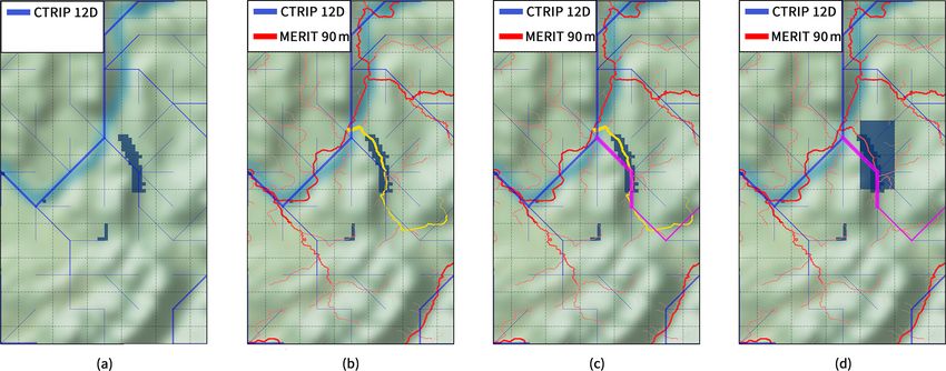
1310                                            T. Guinaldo et al.: Parametrization of a lake water dynamics model MLake

the surface-area-based lower limit, the total number of lakes      cipitation (Pujol et al., 2011; Thiery et al., 2015; Koseki
on Earth ranges from 117 million to 300 million, which rep-        and Mooney, 2019). For example, Bowling and Lettenmaier
resents 3.7 % of the non-glaciated land surfaces (Lehner and       (2010) showed that arctic lakes influence spring peak flow
Döll, 2004; Verpoorter et al., 2014). However, lake density        by storing up to 80 % of the snowmelt water, and simula-
is not evenly distributed on the surface of the globe. Regions     tions over the arctic regions demonstrated a 5 % increase in
like Scandinavia and northern Canada contain the majority          annual mean evapotranspiration over the Great Lakes region
of these water bodies (Downing et al., 2006).                      Mishra et al. (2010). These open-water bodies are large reser-
   Where present, lakes play a triple role in the Earth system,    voirs that generally have peak storage in spring and gradually
affecting the energy and the water budgets of the general cir-     release these volumes to sustain summer low flows. Lake
culation model (GCM) and inducing a modification of the lo-        hydrological effects are size dependent, result in a damp-
cal climate and hydrology (Bonan, 1995; Mishra et al., 2010;       ing of flood waves in terms of magnitude and temporally
Krinner et al., 2012).                                             shift the variability (Spence, 2006). Water dynamics inherent
   First, they influence the atmospheric boundary layer as op-     to lakes are driven by their water balance and consequently
posed to riparian land in terms of surface energy storage.         by their level variations. These key variables affect most of
In addition, lakes influence the freshwater flux variability,      the internal lake processes and control their interactions with
which in the end interacts with the local (Sauvage et al.,         other hydrological components. Historical and projected lake
2018) and global ocean circulation (Rahmstorf, 1995). More-        level drops or increases have been documented (Rodell et al.,
over, the inclusion of the representation of lake fluxes into      2018; Wurtsbaugh et al., 2017) and have led to modifications
numerical weather prediction models can lead to the reduc-         of internal processes such as lake mixing regimes and re-
tion of forecast errors (Balsamo et al., 2012).                    gional water availability (Vörösmarty et al., 2010; Woolway
   Second, as sentinels of climate change, lakes must be seen      et al., 2020).
not only as water reservoirs but also as a major ecological           Lakes have long been considered as a discontinuity within
levers. They reduce the adverse biodiversity footprint caused      the river network, but there is a general agreement now that
by climate change by acting as carbon sinks (Williamson            consideration of the rivers and lakes as a continuum is re-
et al., 2009; Jenny et al., 2020). Multiple studies have demon-    quired (Jones, 2010). Therefore, lakes must be taken into ac-
strated the climate influence on lake surface temperatures         count in global climate change impact studies as populations
(Wagner et al., 2012; Palmer et al., 2014; Sharma et al., 2015;    depend on their inherent ecosystem services (e.g., drinking
O’Reilly et al., 2015). This is important since surface tem-       water, fishing, tourism and leisure. Schallenberg et al., 2013).
perature impacts the lake ecosystem and drives the inherent        Multiple studies have expressed the regional (Ogutu-Ohwayo
lake heat budget and thus the lake mixing regimes (Woolway         et al., 1997; Smith et al., 2015; Zhang et al., 2016) and global
and Merchant, 2019). The large majority of lakes are located       (Janse et al., 2015; Goudie, 2018) threat impacting lakes, and
at high latitudes, which is where air temperatures have risen      they reveal the direct and indirect influence of human ac-
more than the global average over the last century (Hartmann       tivities on biodiversity. The global interest in lakes has led
et al., 2013). This change retroactively affects the regional      the scientific community to make an effort to warn society
climate characterized by a warming effect in autumn and            about the rapid degradation of large lakes worldwide (Jenny
winter and a cooling effect in spring (Martynov et al., 2012;      et al., 2020). Models are frequently used as the basis for
Samuelsson et al., 2010; Le Moigne et al., 2016). Global cli-      prediction, but development of land surface models (Noil-
mate change also constitutes a great environmental threat:         han and Planton, 1989; Krinner et al., 2005; Balsamo et al.,
volumes of several lakes, among which are the Great Salt           2009) and river-routing models intended for large-scale ap-
Lake (USA), Lake Chad (Chad, Cameroon) and Lake Ur-                plications (Vörösmarty et al., 1989; Hunger and Döll, 2008)
mia (Iran), have shrunk significantly and lead to local and re-    have been generally focused on overland flow, groundwater
gional health disasters (Wurtsbaugh et al., 2017; Gross, 2017;     representation and river routing, with less attention on lateral
Pham-Duc et al., 2020). Increasing surface temperature and         fluxes (Davison et al., 2016). Among these, there was a lack
human pressure on lakes reduces freshwater supply and its          of consideration of lake water mass dynamics (Gronewold
quality, disrupting in turn the biological and physical equi-      et al., 2020) because of both the coarse resolution of global
librium through contaminant pollution or reduced freshwater        models and the associated increased computational costs.
storage (Williams, 1996; Cai et al., 2016; Eriksen et al., 2013;   Global climate models (GCMs) usually consider lake energy
Codling et al., 2018; Rodell et al., 2018).                        budget without giving much importance to river–lake con-
   Third, lakes interact with the regional-scale water fluxes      nectivity, even if key regions in climate studies such as Scan-
by increasing the potential over-lake evaporation and lower-       dinavia and northern North America are mainly dependent on
ing the inter-annual and seasonal variability of downstream        this. Global hydrological models (GHMs) usually represent
discharge (Mishra et al., 2010; Bowling and Lettenmaier,           lakes as large rivers with modified characteristics in order to
2010; Cardille et al., 2004). As a secondary moisture source       retrieve the correct downstream river discharge. To address
they can influence regional-scale climate (Krinner, 2003;          the comprehensive outcomes resulting from long-term water
Dutra et al., 2010; Samuelsson et al., 2010) and local pre-

Geosci. Model Dev., 14, 1309–1344, 2021                                            https://doi.org/10.5194/gmd-14-1309-2021
T. Guinaldo et al.: Parametrization of a lake water dynamics model MLake                                                       1311

Table 1. Land surface model integrating a mass balance lake           scribed in detail in Decharme et al. (2019), CTRIP is now
parametrization.                                                      one of the only global model representing the joint effect of
                                                                      floodplains and groundwater on the surface water and energy
 Model name                       Reference                           budget in a climate model. However, the representation of
 Community land model             Oleson et al. (2010)                lakes in the model is limited to the energy budget computa-
 Variable infiltration capacity   Bowling and Lettenmaier             tion by the bulk model FLake (Mironov, 2008), which does
                                  (2010), Mishra et al. (2010)        not take lake mass fluxes into consideration.
 LISFLOOD                         Burek et al. (2013), Zajac et al.      The purpose of the study is to implement lake processes in
                                  (2017)                              the CTRIP river-routing model. This paper will examine the
 MESH                             Pietroniro et al. (2007)            impact of introducing this non-calibrated lake model MLake
                                                                      (Mass-Lake model) at the global scale on river discharge. It
                                                                      will also assess the performance of retrieving correct water
                                                                      storage variations by comparing observed and simulated lake
cycle evolution, GHMs need to characterize every key com-             level variations. To do so, MLake has been implemented in
ponent interacting with each other (Gronewold et al., 2020).          the more recent CTRIP river-routing model at a resolution of
   In recent years many studies have focused on anthro-               1/12◦ , which is the upper limit in resolution for the physical
pogenic open waters (Hanasaki et al., 2006; Haddeland et al.,         processes in the current CTRIP model (otherwise, changes to
2006; Gao et al., 2012), with less attention devoted to the           the module formulation and introduction of hydrodynamic
understanding of natural lake global influence on the global          processes would likely be necessary). Within the system,
water cycle. All of this advocates for a realistic representa-        ISBA simulates runoff and drainage in response to atmo-
tion of lake mass balance in climate studies in order to study        spheric forcing, while CTRIP, the river-routing model, trans-
their role in the global water budget in addition to flood risk       fers water through the hydrographic network of the resolved
management, drought predictions and in helping stakehold-             watersheds. Note that there are challenges to evaluating such
ers to implement realistic policies in water resource manage-         a new model, since global lake datasets remain scarce or in-
ment. To our knowledge, only a few models consider specific           complete. This is mainly explained by the extensive detailed
processes driving lake mass balance (Table 1). These models           field measurements required, such as bathymetry profiling,
have been used for improving flood forecasting (Zajac et al.,         and the associated costs (Hollister and Milstead, 2010). This
2017), assessing the impact of lakes on river streamflows             study tries to overcome these limitations by using inherent
(Huziy and Sushama, 2017), and understanding the impact               CTRIP parameters like the river channel width at the lake
of open-water bodies in the regional water cycle (Bowling             outlet, which obviously leads to uncertainties. Sensitivity
and Lettenmaier, 2010). The main outcome of these stud-               tests are done by prescribing different outlet width configura-
ies is the necessity of implementing lakes in a hydrological          tions and then studying their impact on both the river stream-
model, as they affect both the regional and global water trans-       flow and the lake level amplitude and variability for multiple
fer. Nonetheless, even the latest research efforts remain at a        study sites.
coarse resolution, which limits the number of lakes that can
be represented. These models are often calibrated in order
to retrieve local water patterns, which limits their ability to       2     Modeling framework
implement such schemes at the global scale. Finally, to our
knowledge, no mass balance lake models are effectively inte-          2.1    ISBA-CTRIP system
grated within the land surface system for use in climate mod-
eling and global hydrological applications.                           The ISBA-CTRIP system (https://www.umr-cnrm.fr/spip.
   As one of the contributors to the Intergovernmental Panel          php?article1092; last access: 1 September 2020; Decharme
on Climate Change (IPCC), Météo-France’s Centre National              et al., 2019) simulates the surface energy and water bud-
de Recherche Météorologiques (CNRM) is in charge of                   gets for large-scale climate and hydrological applications. A
the development of the climate model called CNRM-CM                   schematic of this coupled model is shown in Fig. 1. Spatially
(CNRM-Climate Model), the sixth version of which has been             distributed, this model has been evaluated globally in offline
released (Voldoire et al., 2019). This climate model contains         mode (i.e., decoupled from the atmosphere and forced at the
an improved representation of the coupled thermal and hy-             upper boundary using an optimal blend of observations and
drological processes of the land surface called ISBA-CTRIP            numerical weather prediction output) using two sets of at-
(Decharme et al., 2019). This system is based on the coupling         mospheric forcings against in situ measurements and satel-
between the Interaction-Sol-Biosphère-Atmosphère (ISBA)               lite products. The most significant results show improve-
land surface model (Noilhan and Planton, 1989) and the                ments in the river discharge simulations, the snowpack repre-
CNRM version of the Total Runoff Integrating Pathways                 sentation and the land surface evapotranspiration (Decharme
(CTRIP) river-routing model (Oki and Sud, 1998; Decharme              et al., 2019). Recently, the updated version of ISBA-CTRIP,
and Douville, 2007). Thanks to recent developments de-                considering improvements such as wildfires and land cover

https://doi.org/10.5194/gmd-14-1309-2021                                                Geosci. Model Dev., 14, 1309–1344, 2021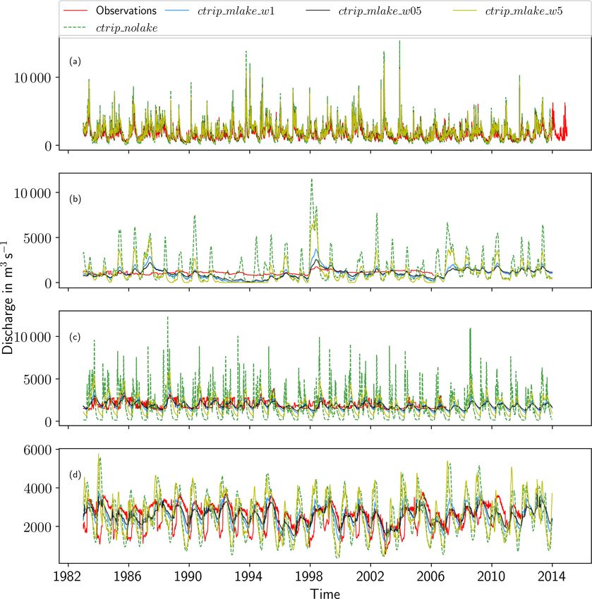
1312                                            T. Guinaldo et al.: Parametrization of a lake water dynamics model MLake

Figure 1. Scheme representing the models in the CNRM Climate Model 6 and the processes integrated in CTRIP, adapted from Decharme
et al. (2019). The processes represented by the CTRIP model are delimited by the blue domain.

changes (Séférian et al., 2019), has also shown a better rep-      land processes in SURFEX comes from the global land cover
resentation of global-scale carbon pools and fluxes (Delire        database ECOCLIMAP-II, which dynamically renders the
et al., 2020).                                                     type of vegetation and its cover at the chosen spatial reso-
   Originally the land surface model ISBA simulated sev-           lution of the model for a given application (Masson et al.,
eral key land surface variables, such as surface runoff or         2013; Faroux et al., 2013).
soil moisture, in response to atmospheric forcings based on           ECOCLIMAP-II is a 1 km resolution land use and land
a force-restore approach. This scheme represents land pro-         cover database based on satellite products designed for op-
cesses as a single soil–vegetation–snow continuum, limiting        erational and research numerical weather prediction, cli-
the prediction of root layer droughts and the heterogeneity        mate modeling, hydrological forecasting, and in land sur-
of soil properties. Currently, the diffusive version of ISBA       face numerical studies within the SURFEX surface model-
is used for hydrological and climate modeling applications.        ing platform (Le Moigne et al., 2009). ECOCLIMAP-II de-
It explicitly resolves both the one-dimensional Fourier and        tails whether a pixel contains one of the four different type
Darcy laws for subsurface thermal and mass fluxes, and it ac-      of covers (lake, town, land or ocean), and it distinguishes
counts for the hydraulic and the thermal properties of soil that   hundreds of plant functional types, representing a large va-
is now discretized in 14 layers, resulting in a total depth of     riety of ecosystems (Faroux et al., 2013). SURFEX further
12 m. In addition, the scheme can include the effects of soil      aggregates the initial covers into upwards of 20 patches that
organics on the thermal and hydrological properties of the         correspond to different land covers or plant functional types.
soil. The snow is simulated using a multi-layer snow model         The orography is extracted and upscaled from the 90 m res-
based on the work of Boone and Etchevers (2001) with recent        olution Shuttle Radar Topography Mission to a 1 km resolu-
improvements in physics and increased vertical resolution as       tion (Werner, 2001). The ECOCLIMAP-II lake cover scheme
described in Decharme et al. (2016).                               provides binary information on the presence (or lack thereof)
   ISBA is fully integrated within the surface modeling plat-      of a lake in the pixel. No other information is provided, and
form SURFEX (v8.1) (Masson et al., 2013; Le Moigne et al.,         thus lake cover information is completed with the Global
2020) developed at the CNRM in order to bring all the mod-         Lake DataBase (GLDB, Kourzeneva et al., 2012; Choulga
els related to the surface parametrization into one unique         et al., 2014), which has gridded in situ and estimated lake
software platform. SURFEX allows studies to be performed           mean depth at 1 km resolution globally. This global database
in offline mode or fully coupled to an atmospheric model,          has been developed to gather lake information and retrieve
de facto extending its applicability range from local hydro-       mean depth information for numerical weather prediction.
logical to large-scale climate studies. The distinction of such    It already serves as input for correcting land cover used by

Geosci. Model Dev., 14, 1309–1344, 2021                                            https://doi.org/10.5194/gmd-14-1309-2021
T. Guinaldo et al.: Parametrization of a lake water dynamics model MLake                                                    1313

SURFEX for approximately 15 000 lakes on a 1 km resolu-           order SNdownstream attribution follows the following rule:
tion grid. However, a dataset threshold is introduced on lake
detection and set at a surface area of 1 km2 that limits the      SNdownstream = max(SNi,upstream ) + 1, i ∈ [1, N ],          (1)
number of lakes considered in our calculations. In this re-       where SNi,upstream represents the sequence number of the up-
search, we used continuous mean depth field recently devel-       stream river, i, and SNdownstream is the sequence number of
oped at ECMWF (Choulga et al., 2019) to ease aggregation          the downstream river.
technique from 1 km to 1/12◦ .                                       The main motivation for the integration of new processes
   Streamflow routing is simulated using CTRIP (Fig. 1),          in CTRIP is to both simulate river discharge and to enable
which integrates a dynamic computation of river flows based       the quantification of the impact of climate change on drought
on a kinematic wave approximation that is solved using Man-       and flood risk over the entire globe. It is also a valuable tool
ning’s roughness equation as a friction energy dissipation        that gives estimates of global water resources in the context
term that is dependent on the characteristics of the river sec-   of global depletion. Regarding the global water budget, the
tion. CTRIP is fully coupled to SURFEX and considers the          ISBA-CTRIP model improves the simulations of both peak
interaction between the rivers, the atmosphere and the soil       discharges and baseflow, in addition to global terrestrial wa-
through the input of CTRIP, which then computes the river         ter storage variations. However, Decharme et al. (2019) ad-
discharge, water table evolution and surface flooded frac-        dressed the need to increase the resolution in order to avoid a
tion. Moreover, it explicitly accounts for groundwater pro-       sub-grid parameterization and in order to consider the water
cesses with the integration of a two-dimensional diffusive        dynamics more precisely. Originally used at a resolution of
aquifer scheme connected to rivers and a parameterization         1◦ , then down-scaled at 0.5◦ , ongoing improvements permit
of the capillary fluxes within the soil (Vergnes et al., 2014).   the model to run at its current resolution: 1/12◦ (approxi-
Descriptions of the parameterization of flooding processes        mately 6–8 km at midlatitudes). This resolution guarantees
can be found in Decharme et al. (2019). The coupling of           a better discretization of surface and subsurface processes
ISBA and CTRIP is made through the OASIS3-MCT cou-                without the need to implement additional river hydrodynamic
pler (Voldoire et al., 2017), where ISBA provides surface         processes. The river network at 1/12◦ has been derived by
runoff and drainage estimates, which are then transformed         applying the Dominant River Tracing algorithm (DRT; Wu
by CTRIP in river discharge, water table height or flood-         et al., 2012) on the high-resolution river network (3 arcsec) of
plain fraction. In addition to the fully coupled configuration,   MERIT HYDRO (Yamazaki et al., 2019). CTRIP parameters
CTRIP can be used in an offline configuration forced by the       describing river properties and floodplain and aquifer charac-
runoff and drainage coming from ISBA (or other land surface       teristics have been derived following the same methodology
model) simulations and without feedbacks between the water        as for the 0.5◦ version of CTRIP (for details see Decharme
bodies and the soil processes. Further details on the physical    et al., 2019).
processes are presented in Decharme et al. (2019).
   In this study, we refer to CTRIP as a global-scale model,      2.2   Flake: a lake energy balance model
meaning that it is a 1/12◦ resolution model applied to areas
ranging from large basins to a domain covering the entire         Lake evaporation is simulated using the FLake model
globe.                                                            (Mironov, 2008). When considered together with the precipi-
   Each CTRIP pixel represents a unique rectangular river         tation, an estimation of water mass exchange by the lake with
section with its own characteristics. As shown in Fig. 2, in-     the atmosphere can be made. FLake is a bulk model capable
stead of working directly with grid cell, each river section      of simulating the lake energy budget within the lake and at
is integrated as a node in the network and all nodes are la-      the lake–atmosphere interface (Mironov et al., 2010). FLake
belled sequentially. Their number defines the position of the     is designed mainly for use in numerical weather prediction
river section in the network for each hydrographic basin. The     and climate studies, where it helps in determining the ver-
scheme increasingly iterates on this number and ensures all       tical lake temperature structure, the mixing conditions, and
the upstream masses have been updated before the numeri-          the retroaction with the local and regional climate (Balsamo
cal computation on a designated node of the network starts.       et al., 2012; Le Moigne et al., 2016; Salgado and Le Moigne,
This numerical solution framework assures the computation         2010). FLake is based on a numerical solution of a two-layer
of river discharge is performed starting from the upstream        parametric evolution of the temperature profile and the inte-
cells and then progressing to the downstream cells of the wa-     gral budgets of heat and kinetic energy. The mixed layer is
tershed. In every basin, the head-water cells have the low-       characterized by a uniform temperature and an entrainment
est sequence order, i.e., one, which is incremented for each      equation that estimates the layer depth. Below this first layer,
downstream cell. The general rules of attribution consider        the vertical temperature profile is parameterized in order to
that a node can receive water from multiple affluents but can     represent the thermocline shape based on a self-similarity
not have multiple downstream sections. Considering the case       concept (Kitaigorodsky and Miropolsky, 1970). This model
of an affluent with multiple upstream nodes and in order to       uses external parameters, of which the most important are the
avoid conflicts at the confluence, the downstream sequence        lake mean depth and the extinction coefficient (set to 0.5 m−1

https://doi.org/10.5194/gmd-14-1309-2021                                            Geosci. Model Dev., 14, 1309–1344, 2021
1314                                             T. Guinaldo et al.: Parametrization of a lake water dynamics model MLake

Figure 2. Graphical representation of the CTRIP algorithm. (a) Spatially distributed network representation for CTRIP only. (b) The same
for CTRIP-MLake.

following Le Moigne et al., 2016). The numerical solution             e.g., Finland. For example, estimated lake mean depth in all
is based on the evolution of four lake prognostic variables,          boreal zones is based on geological method taking into ac-
i.e., the surface temperature, the lake bottom temperature,           count a tectonic plate map and geological maps (Choulga
the thickness of the mixed layer, and the shape factor, and           et al., 2014). The geological method assumes that lakes of
one parameter, i.e., the mean lake depth. An extensive de-            the same origin and region should have the same morpholog-
scription of the model can be found in Mironov (2008).                ical parameters, e.g., mean depth. In our study small lakes
                                                                      tend to be aggregated as a unique larger lake that might not
2.3     MLake: a global scale mass balance lake model                 represent the local morphology. These anomalies can mod-
                                                                      ify the local hydrology; however, considering the scale of the
2.3.1    Generation of a global lake mask                             current study, these effects are limited or even can be filtered
                                                                      by averaging.
Before implementing the numerical representation of lake
dynamics into the CTRIP model, lakes need to be introduced            2.3.2   Integration of lakes in the river-routing model
in the river network at 1/12◦ . However, the ECOCLIMAP-II                     (RRM)
provides binary information of the lake detection at 1/120◦ ,
meaning the information needs to be upscaled to the CTRIP             At the model resolution of CTRIP, a unique river stretch is at-
resolution. The method is based on a recursive aggregation of         tributed to each grid cell. Replacing a river pixel with a lake
neighboring lake pixels, which depends on the GLDB mean               follows the same logic as water transfer, which is dependent
depth. In other words, for every pixel at 1/120◦ , the algo-          on the riparian topography and its location within the water-
rithm scans the surrounding pixels and aggregates those that          shed. However, integrating a lake which can cover more than
are connected and have the same mean depth. Each aggre-               one grid cell in the CTRIP river networks is not straightfor-
gated lake is then identified with a unique number used fur-          ward. Huziy and Sushama (2017) proposed a distinction be-
ther when attributing inherent parameters and variables.              tween local lakes, covering at least 60 % of a grid cell, and
   This method is developed for large lake identification but         global lakes, which can cover several grid cells. This distinc-
struggles in the regions with a high density of small lakes,          tion brings some dynamic limitations as a local lake can only

Geosci. Model Dev., 14, 1309–1344, 2021                                                 https://doi.org/10.5194/gmd-14-1309-2021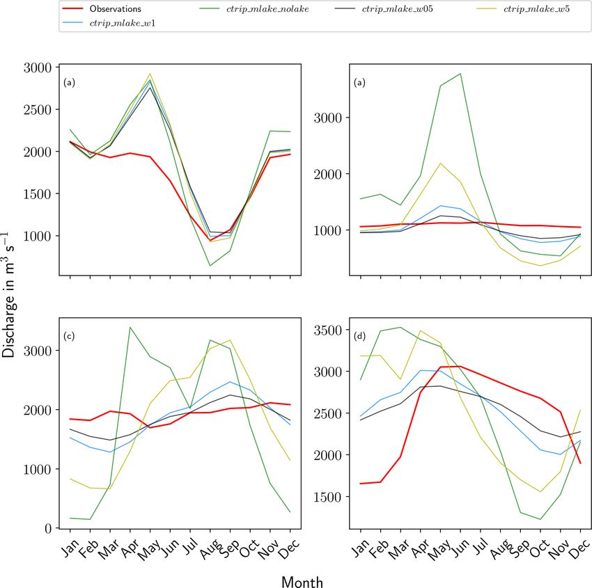
T. Guinaldo et al.: Parametrization of a lake water dynamics model MLake 1315
Figure 3. Procedure for the integration of a lake in the CTRIP river network at 1/12◦ resolution. An example is given for Lake Bourget
(France). Panel (a) presents Lake Bourget at a 1/120◦ resolution and the CTRIP river network at a 1/12◦ resolution. Panel (b) shows the
identification of the river stretch from the MERIT HYDRO river network covered by the lake pixels. Panel (c) presents the selected river
stretch in the CTRIP 1/12◦ . Panel (d) shows the lake network mask at a 1/12◦ resolution resulting from the recursive identification using
MERIT HYDRO.
are located on a pixel. At the 1/12◦ , a lake can cover a small
fraction of the pixel while being actually part of another
watershed. This is the case for the Lake Bourget (France,
Fig. 3a), where a river that flows on another watershed con-
tains most of the runoff of the pixel while the lake only cap-
tured a small amount of water that is part of the lake wa-
tershed. The other issues concern the location of the lake in
the river network and which river stretch is actually a part
of lake. In some regions, the river stretch can be large and
thus the streamflow time response remains slow, which can
be close to the response time of a lake. Consequently, finding
a compromise between the lake spatial extension at different
resolutions and the actual lake water dynamic is important.
The approach used herein to resolve this issue is to replace
a river section with a lake pixel (corresponding to a unique
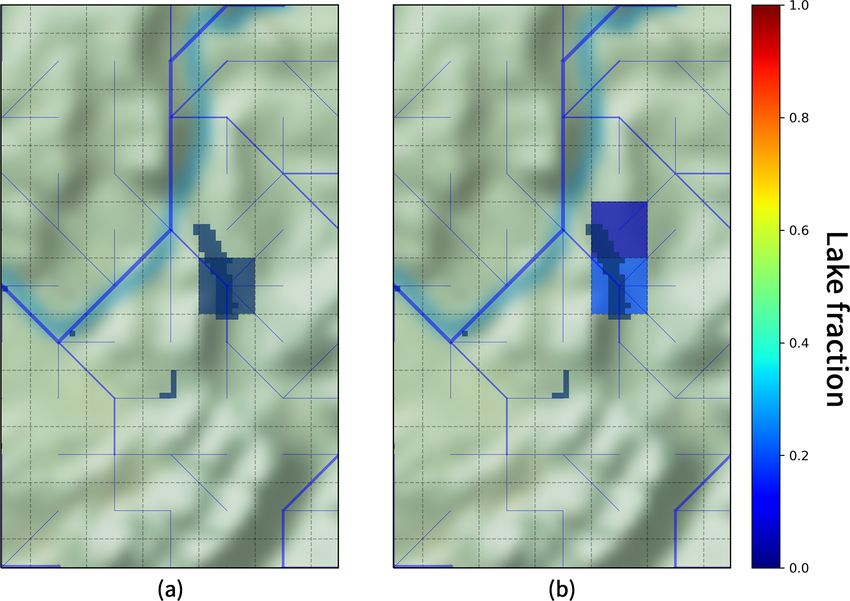
Figure 4. Example of a network (a) and runoff (b) masks for Lake node in the network) when a lake covers at least 50 % of a
Bourget (France). given grid cell (Fig. 2). Wherever a lake spreads over sev-
eral grid cells, two distinct lake masks are necessary. This is
important, on the one hand, to ensure that the water flux re-
be an extension of the river section that contributes to the mains realistic and, on the other hand, as the introduction of
downstream flow without being fed by the river itself. On the lake mass dynamics should not significantly change the local
contrary, a large lake is part of the river network and divides hydrology.
the river in an upstream section that contributes to the total First, a lake mask, called the “network mask”, is needed
lake inflow and a downstream section connected to the lake to locate the lake within the river network and to link the
that receives its mass from the lake outlet. However, it is im- considered lake to the correct river. The procedure of this in-
portant to keep a unique method that can adapt to all lakes tegration is based on the steps presented in Fig. 3. In CTRIP,
regardless of their size. an identification number is assigned to every river that al-
Some issues related to the integration of lakes in the river lows a distinction between rivers of the same watershed. This
network emerge when considering that lakes add a spatial identification number comes from the upscaling of the 90 m
dimension to the network linked to the fraction of pixel cov- resolution MERIT HYDRO (Yamazaki et al., 2019). The up-
ered. First, the model must estimate a correct partitioning of scaling of the river network from 90 m to 1/120◦ resolution
the runoff between rivers and lakes when both components
https://doi.org/10.5194/gmd-14-1309-2021 Geosci. Model Dev., 14, 1309–1344, 2021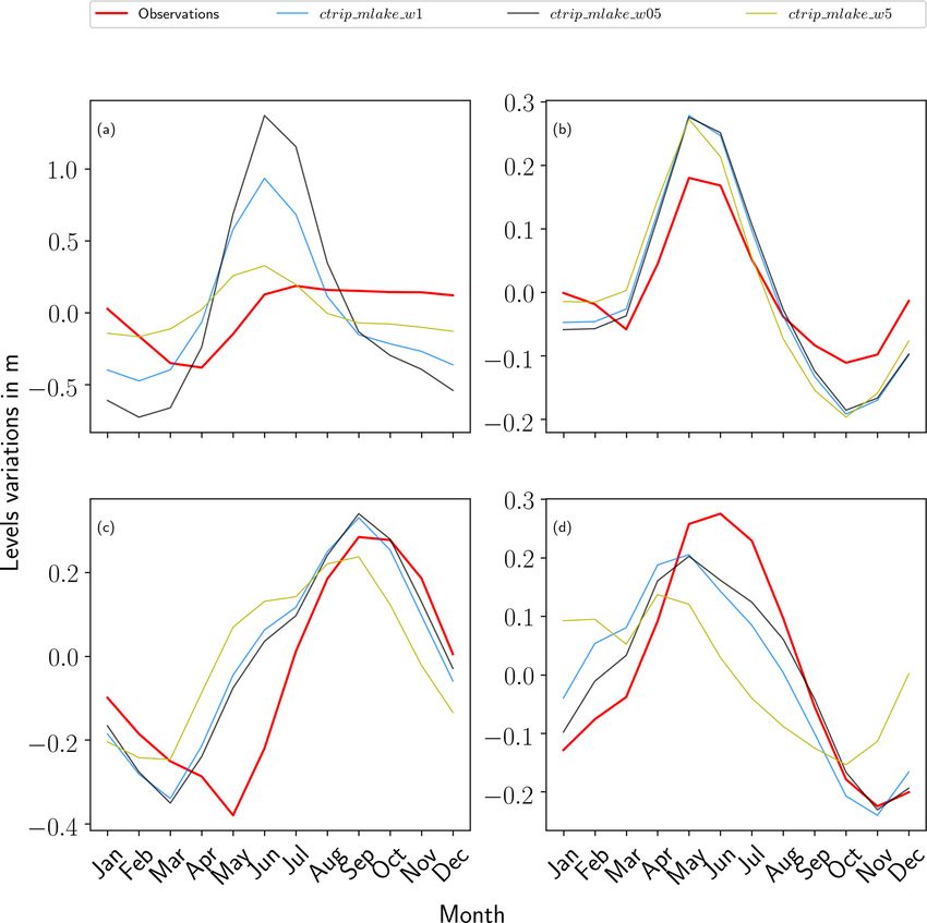
1316                                              T. Guinaldo et al.: Parametrization of a lake water dynamics model MLake

Figure 5. Schematic representing the process participating in a lake mass balance evolution.

preserves the continuity of this ID number. Identification of              Thus, a second lake mask is needed: the lake runoff mask.
lake pixels follows the same rules. To do so, a function recur-         The runoff mask creation is based on the lake information
sively determines every lake pixel at a 1/120◦ resolution that          coming from ECOCLIMAP at 1/120◦ resolution as pre-
covers a river stretch of the MERIT HYDRO river network                 sented in Fig. 4b. In fact, this runoff mask corresponds to
with the same identification number as the river that flows             every CTRIP pixel at the 1/12◦ resolution that contains at
at the outlet (river stretch identified in yellow in Fig. 3b).          least one ECOCLIMAP lake pixel (at the 1/120◦ resolution).
Thereby, all lake pixels are linked to the correct river ID num-        In other words, this is a mask of the lake fraction at 1/12◦
ber and this link is preserved while upscaling to the 1/12◦             without any distinction of the watershed or the lake fraction.
resolution (Fig. 3d). The network mask ensures that all of              It provides information on the spatial extension of the lake
the lake pixels with the same ID number are coupled within a            within the river network, and it is used for computing the wa-
unique mass balance process. However, as shown in Fig. 3d,              ter mass intercepted by the lake from the land surface models
a few conflicts may appear while applying this method. In               (as runoff and drainage).
this particular example, the northern pixel is not part of the
lake’s watershed and flows out within another basin, which              2.3.3   Lake model
induces a conservation issue. A second function recursively
determines every lake pixel at a 1/12◦ resolution that cov-             The MLake mass balance equation is based on the differ-
ers a river stretch of the CTRIP river network (river stretch           ence between the mass fluxes entering and leaving the lake
identified in pink in Fig. 3d). This last step ensures the lake         (Fig. 5). At each time step, the lake module calculates the
network only considers lake pixels that are effectively in              prognostic net water storage Vlake (kg) over the lake surface
the river basin. The lake network mask for Lake Bourget is              area based on the following equation:
shown in Fig. 4a. At the end of each time step, diagnostic              dVlake
variables are distributed on this mask. This method ensures                    = Pol − Eol + R + D + Qin − Qout − Qgw ,             (2)
                                                                         dt
all freshwater lake pixels are effectively linked to the correct
river within the entire network and that water mass flowing             where t is the time (s), Pol is the over-lake precipitation
in a different watershed is not entering the lake.                      term (kg s−1 ), Eol is the over-lake evaporation term (kg s−1 ),
                                                                        R and D are terms to account for runoff and drainage, re-
                                                                        spectively, as estimated by ISBA (kg s−1 ) over the runoff

Geosci. Model Dev., 14, 1309–1344, 2021                                                   https://doi.org/10.5194/gmd-14-1309-2021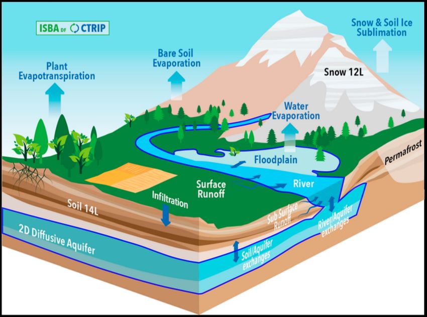
T. Guinaldo et al.: Parametrization of a lake water dynamics model MLake 1317
Figure 6. Lake–river interaction through overflows.
mask, Qin is the inflow entering the lake from the tribu- of such interactions at a larger scale can be difficult owing to
taries (kg s−1 ), Qout is the lake outflow (kg s−1 ), and Qgw a lack of understanding of the processes involved. As a con-
represents the contribution of the lake–groundwater fluxes sequence, only groundwater–river processes already present
(kg s−1 ). in the model are activated, meaning there is no interaction
The mass balance equation is numerically resolved in two between groundwater and lakes that will be integrated in a
steps: first, an estimate of the incoming flows is computed further version of MLake.
and used to define an intermediate lake volume Vlake ∗ . Next, As mentioned previously, the outflows are calculated con-
the outgoing water flow is estimated based on this intermedi- sidering an intermediate lake state in order to retrieve the fi-
ate state in order to return to a new lake equilibrium state. In- nal lake volume. This intermediate state for the time step (s)
coming flows consist of contributions from both the riparian is defined as an intermediate volume Vlake∗ (kg):
banks and the direct river inflows. The riparian bank runoff
∗
and drainage volumes are collected by the lake and computed Vlake (t) = V (t − 1t) + [Pol (t) − Eol (t) + RS (t)
over the runoff mask as shown in Fig. 4 following the follow- +Qsub (t) + Qin (t)] 1t (5)
ing rules:
P where 1t is the time step (s) and V (t −1t) is the lake volume
R = rS (p)
at the previous time step t − 1t (kg s−1 ). Equation (6) pro-
p
P (3) vides an estimation of the intermediate lake hydraulic head
D = dS (p),
h∗lake (m):
p
∗ (t)
Vlake
where rS and dS represent the runoff and drainage fluxes,
h∗lake (t) = , (6)
respectively, over the pixel p on the runoff mask ω. The spe- AECO
cific inflows flowing into the lake are composed of all the up-
stream tributaries (with a lower sequence number) connected where AECO is the lake area in the ECOCLIMAP-II database
the network mask following the following equation: (m2 ).
The outflow is, by definition, linked to the lake water stor-
l
X age assuming a rating curve relation based on an empirical
Qin = qin (k), (4) weir relationship that links the discharge to the water head
k
over the crest (Eq. 7). The outflow starts as soon as the lake
where qin is the river discharge of the tributary number k height exceeds the weir height. The discharge is then a func-
and l is the total number of tributaries for the considered tion of a hydraulic head, which represents the height of wa-
lake. Even if it is not applicable for long-term hydrologi- ter above the weir. This approach mimics the lake outlet dy-
cal analysis, due to a lack of knowledge on the large-scale namic as a waterproof basin that flows out through a counter-
process, the groundwater flux is often the missing term indi- slope. The need to model outflow at the global scale restricts
rectly retrieved from the residuals of the mass balance com- the complexity of the parametrization, as it needs to take into
putation. The lateral and vertical groundwater fluxes are very account all lake types. At the current resolution of the model
sensitive to the spatial resolution (Reinecke et al., 2020). (i.e. 1/12◦ ), the outlet is assumed to be small enough to be
Groundwater–lake interactions are generally better under- considered a straight section connected to the downstream
stood locally (Bouchez et al., 2016), but the representation river without any friction and to have the same shape as the
https://doi.org/10.5194/gmd-14-1309-2021 Geosci. Model Dev., 14, 1309–1344, 2021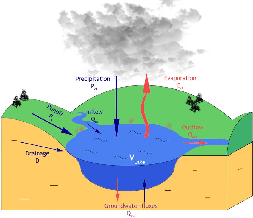
1318                                                   T. Guinaldo et al.: Parametrization of a lake water dynamics model MLake

downstream rectangular river section. This approach is rep-                  3   Study sites
resented in Fig. 6.
   The outflow is calculated as follows:                                     Four watersheds have been selected in order to assess the
                                                                             impact of lakes on regional-scale hydrology. A map showing
             0                                   if h∗lake ≤ hweir

Qout =         √                             3                         (7)   the location of the basins is presented in Fig. 7. They have
             Cd 2gWweir ρω (h∗lake − hweir ) 2   if h∗lake > hweir ,
                                                                             been chosen based on several criteria: their size, their local-
where Cd a dimensionless coefficient related to the drag of                  ization in the drainage basin, and their climate characteristics
the weir, which is prescribed as 0.485 (Lencastre, 1963),                    (in order to assess the sensitivity of the model to different
Wweir the width of the outlet equal to the width of the river in             forcing conditions). These characteristics are summarized in
the downstream pixel (m), hweir the height of the weir (m),                  Table 3. The first watershed is the Rhône basin with its out-
and ρω is the volumetric mass of the water (kg m−3 ).                        let located at Beaucaire (France). Flowing from the Furka
   The river width was first determined over France by com-                  glacier in Switzerland to the Mediterranean Sea (Rhône
paring the mean annual discharge measurements from the                       delta), the basin represents 17 % of the French metropoli-
Banque Hydro database (http://www.hydro.eaufrance.fr, last                   tan area. The Rhône is a socioeconomic lever in terms of
access: 4 March 2021) and the river width of the Systeme Re-                 both quantitative (freshwater resource, industrial needs, sail-
lationnel d’Audit de l’Hydromorphologie des Cours d’Eau                      ing, etc.) and qualitative resource management (ecological
(SYRAH), which leads to the following empirical equation                     state, tourism , etc.). In its upstream part, the streamflows are
(Vergnes et al., 2014):                                                      dependent on the glacier water supply, whereas in its down-
                                                                             stream part the Mediterranean climate directly impacts the
               β
ωriver = αQmean ,                                                      (8)   discharge and water level associated with flash flood risks.
                                                                             Therefore, these diverse forcings induce a bi-modal hydro-
where α and β are dimensionless parameters, respectively,                    logical regime. Within this watershed, five lakes are identi-
equal to 5.41 and 0.59 (Vergnes et al., 2014). Qmean is the                  fied at a spatial resolution which must be resolved within the
mean annual discharge of the river calculated over the cli-                  current study, among them is Lake Geneva, which is one of
mate period (1981–2010). This empirical exponential func-                    the largest European freshwater reservoirs, with an average
tion has been extended to the global scale by Decharme                       volume of 89 km3 . With a relatively small drainage area com-
et al. (2019) based on the comparison of two datasets:                       pared to other lakes, Lake Geneva creates a link between the
the Global Width Database for Large Rivers (GWD-LR:                          mountainous upstream and the fluvial downstream regimes.
http://hydro.iis.u-tokyo.ac.jp/~yamadai/GWD-LR/, last ac-                    Located on the upstream part of the Rhône network, it also
cess: 4 March 2021) and the Global Lakes and Wetlands                        controls the streamflows and limits flooding during spring.
Database (GLWD, http://wp.geog.mcgill.ca/hydrolab/glwd/,                     Due to the importance of karstic structures for the down-
last access: 4 March 2021, Lehner and Döll, 2004).                           stream River Rhône and especially the baseflow, this basin is
   The initial lake level is equal to the weir height, which                 the only study site where the groundwater scheme has been
results in an initial lake outflow equal to zero. Equation (7)               activated.
incorporates the dependence of the depth on the hydraulic                       The second watershed is the Angara River basin in Irkutsk
head over the weir. The final lake volume for the time step                  (Russia). The water mass flowing from Lake Baikal controls
(t) is derived from the following equation:                                  the streamflows of the Angara watershed, which flows to its
                                                                             confluence with the Yenisey River at Strelka. This watershed
              ∗                                                              was selected in order to study the specific hydrological con-
Vlake (t) = Vlake (t) − Qout (t)1t.                                    (9)
                                                                             ditions of Lake Baikal, the waters of which freeze in win-
Equation (2) calculates a change in lake water storage from                  ter, and its prevalence on the regional hydrological system.
which the diagnostic variables, such as surface area and lake                Known both for its unique endemic ecosystem and its mor-
level, are estimated. Numerous hydrological models assume                    phometric characteristics, Lake Baikal is the deepest lake in
the lake storage to be a linear function of the surface area and             the world (maximum depth of 1632 m) and the second largest
depth. This solution does not take into account the specific                 lake in terms of volume (approximately 23 600 km3 ). One of
lake bathymetry, and it simulates a realistic hypsographic re-               the lake’s characteristics is its surface freezing period (ap-
lation; thus, the lake surface area is assumed to be constant.               proximately 5 months), which contributes to its specific hy-
However, knowing how the lake surface area varies with re-                   drological regime.
spect to depth is important for improving over-lake evapo-                      The third watershed is the upstream part of White Nile
ration estimations. With regards to the relative scarcity of                 River in Jinja (Uganda). Characterized by a dry continental
global-scale datasets on lake bathymetry, implementing ap-                   climate, the White Nile originates from the outflow of Lake
propriate lake hypsometric curves would require extensive                    Victoria, which is the world’s second largest lake in terms of
developments that will be carried out in further studies. For                surface area (69 485 km2 ). In contrast to lakes such as Lake
simplicity, in the current study hypsometric curves are as-                  Baikal, Lake Victoria has a relatively small drainage area
sumed to be linear.                                                          (167 000 km2 ), and its water balance is driven mainly by the

Geosci. Model Dev., 14, 1309–1344, 2021                                                        https://doi.org/10.5194/gmd-14-1309-2021
T. Guinaldo et al.: Parametrization of a lake water dynamics model MLake 1319
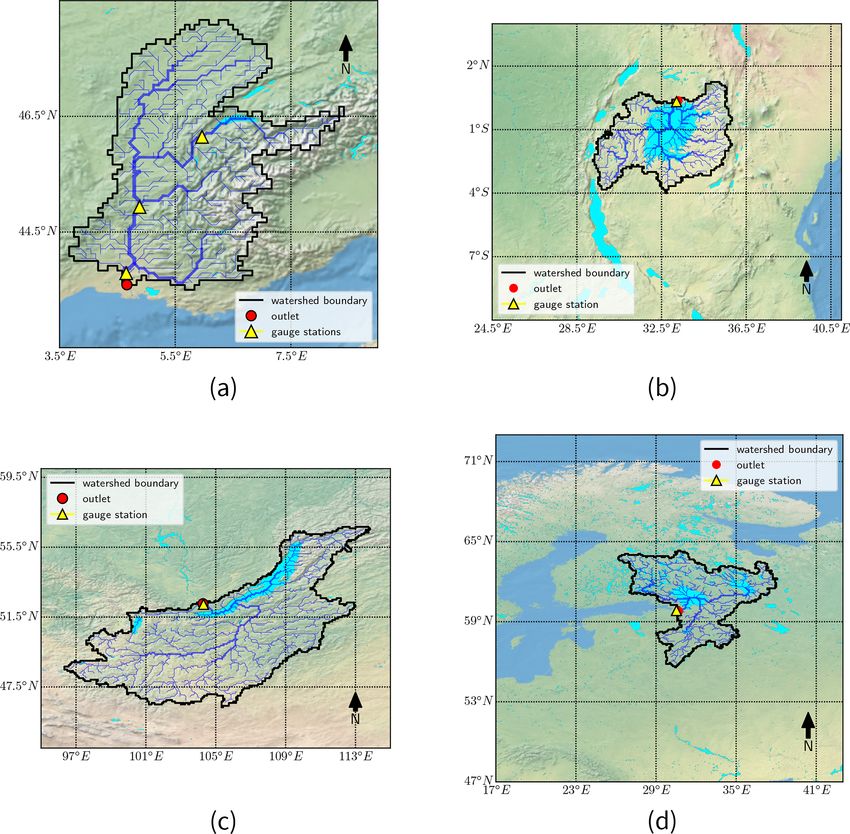
Figure 7. Location of the study sites chosen for the validation of the MLake model: (a) Rhône, (b) White Nile, (c) Angara and (d) Neva.
Made with Natural Earth topographic maps.
precipitation and evaporation (Vanderkelen et al., 2018). Sur- The last watershed is the Neva River basin close to Saint
rounded by the Great Rift Valley, it is a major socioeconomic Petersburg (Russia). This relatively small river (74 km) is the
resource that directly supplies 30 million people and indi- main outlet of Lake Ladoga, the largest European lake. The
rectly supplies over 300 million people living near the Nile. Neva is influenced by the Svir River, at the outlet of Lake
Since 1951, the outflow has been regulated by the Nalubaale Onega, which is the second largest European lake. The sur-
Dam, with a second dam also being built in the 1990s by face area of these lakes are 17 800 and 9800 km2 (Filatov
the World Bank. However, the regulation is controlled by an et al., 2019), respectively. The Ladoga hydrographic basin
“agreed curve”, which intends to mimic natural outflow and is complex and represents dozens of lakes that buffer the
links the water releases to the lake levels. streamflows within the basin. In addition, these lakes are lo-
cated in the boreal zone, which are regions where the positive
https://doi.org/10.5194/gmd-14-1309-2021 Geosci. Model Dev., 14, 1309–1344, 20211320 T. Guinaldo et al.: Parametrization of a lake water dynamics model MLake
Table 2. Lake parameters and variables introduced in CTRIP scripts.
lake_id – lake id number on the runoff mask
lake_net_id – lake id number on the network mask
frac_lake – lake fraction on every CTRIP 12D pixel grid
Parameters z_mean m lake mean depth from GLDB database
a_lake m2 lake surface area from ECOCLIMAP-II
weir_z m crest height at the lake outlet
weir_w m lake outlet width
lake_sto kg lakes storage
Variables lake_h m lake level height over the mean initial depth
lake_out kg s−1 lake outflows over the weir
Table 3. Description of the study site chosen for the evaluation of MLake.
Watershed 1: Rhône
Basin name Rhône
Outlet chosen Beaucaire (France)
Drainage area 97 800 km2
Number of lakes considered 5
Main lake Lake Geneva
Köppen–Geiger climate classification for the main lake Cfb (temperate continental climate with cool humid
winter and relative cool summer)
Watershed 2: Angara
Basin name Angara
Outlet chosen Irkutsk (Russia)
Drainage area 577 000 km2
Number of lakes considered 9
Main lake Lake Baikal
Köppen–Geiger climate classification for the main lake Dwb (cold continental climate with dry winter and tem-
perate summer)
Watershed 3: White Nile
Basin name White Nile
Outlet chosen Jinja (Uganda)
Drainage area 167 000 km2
Number of lakes considered 1
Main lake Lake Victoria
Köppen–Geiger climate classification for the main lake Af (equatorial climate)
Watershed 4: Neva
Basin name Neva
Outlet chosen Saint Petersburg (Russia)
Drainage area 97 800 km2
Number of lakes considered 5
Main lake Lake Ladoga
Köppen–Geiger climate classification for the main lake Dfb (warm summer continental climate)
air temperature anomalies are the largest. Ladoga remains atures of the lakes, specifically those from Lake Onega, are
partly ice free until early winter (the freezing season extends sensitive to atmospheric changes because of their relatively
from November until the end of May), and therefore it has low heat capacity (Filatov et al., 2016). The Ladoga drainage
a significant impact on the regional meteorological condi- area is approximately 97 800 km2 and that of Lake Onega is
tions, such as the enhancement of severe convective snowfall 51 540 km2 . These lakes are particularly affected by changes
episodes (Eerola et al., 2014). In response, the water temper- in river runoff, and studies show a decline in the lake levels
Geosci. Model Dev., 14, 1309–1344, 2021 https://doi.org/10.5194/gmd-14-1309-2021T. Guinaldo et al.: Parametrization of a lake water dynamics model MLake 1321
owing mainly to a regulation of its flows (Hanasaki et al., topographic variability over France. This limits the compari-
2006) and complex interactions with permafrost thawing due son between watersheds situated in France and other basins,
to climate change (Karlsson et al., 2015). but it gives more credit to the results between similar water-
sheds.
4 Materials and data 4.2.1 Reanalysis over France
4.1 Lake observations and discharge data
SAFRAN-ISBA-MODCOU (SIM, Habets et al., 2008;
Model lake level validation is based on the comparison of Le Moigne et al., 2020) is a hydrometeorological model sys-
simulations with multi-mission satellite measurements. The tem that results from the collaboration between the CNRM
elevation data come from the Hydroweb platform (avail- and Mines ParisTech (Etchevers et al., 2001). The system is
able at: http://hydroweb.theia-land.fr/?lang=fr&, last access: composed of the meteorological analysis system SAFRAN
4 March 2021, Crétaux et al., 2011). This platform pro- (Durand et al., 1993; Quintana-Segui et al., 2008), the land
vides, with centimetric accuracy, user-friendly altitude mea- surface model ISBA and the hydrogeological model MOD-
surements for approximately 1000 sites for major rivers and COU (Ledoux et al., 1989).
approximately 230 lakes dating back to 1993. In addition, SAFRAN provides an analysis, based on optimal inter-
Hydroweb provides lake surface extent and volume varia- polation, of near-surface variables such as daily precipita-
tions in several areas worldwide. tion, 2 m relative humidity, 2 m air temperature, 10 m wind
Some lakes are not monitored from space, and thus in situ speed, cloudiness, and model visible and infrared radiative
measurements remain the most accurate source of informa- fluxes. The ISBA model is driven offline by SAFRAN analy-
tion. In the case of Lake Geneva, data from three measure- sis, and it computes the energy and water budgets in order to
ment sites were provided by the EAWAG/EPFL institute and generate surface runoff, total evapotranspiration, soil mois-
the Swiss Environmental Office. These observations cover ture and drainage at an 8 km horizontal resolution. MOD-
the time period 1973 to 2013 and are used to monitor the COU uses surface runoff and drainage as inputs for river-
level variations of Lake Geneva on three different shores. routing and aquifer water head simulations, respectively,
Regarding discharge data, a comparison was made with over all of France. SIM also needs physiographic parame-
a dataset comprised of data from the Global Runoff ters that describe the land cover, soil texture and orography
Data Center (GRDC; http://www.bafg.de/GRDC/EN/Home/ of the studied zone. These parameters are provided by the
homepage_node.html, last access: 4 March 2021), ARCTIC- ECOCLIMAP-II database.
NET and the French Banque Hydro databases (http://www. This physically based system has several applications in
eaufrance.fr, last access: 4 March 2021). From these datasets, operational, research and climate services: it is used in flood
chosen stations must have a minimum of 3 years of con- risk forecasting, water resource management and climate
tinuous measurements during the simulation period for a projections (Soubeyroux et al., 2008). Further details about
drainage area covering at least 1000 km2 . In the validation the model can be found in Le Moigne et al. (2020). For the
stage, the most downstream measurement station is chosen current study, SAFRAN and ISBA have been used to retrieve
for comparison. However, if only one station is available surface runoff and soil drainage estimations for each CTRIP
for the entire study site, the closest available CTRIP pixel pixel of the Rhône watershed over the period 1958–2016.
on the river is considered. These datasets remain incomplete
and some basins lack data, such as the White Nile water- 4.2.2 Global-scale atmospheric variables
shed. The Lake Victoria watershed does not have any ac-
cessible discharge measurement sites. In this particular case, Uncertainties associated with the forcing variables are com-
outflow measurements from Vanderkelen et al. (2018), who monly quantified by using a set of multiple atmospheric forc-
studied Lake Victoria water balance from the Jinja Station, ings. For example, (Decharme et al., 2019) used two state-
were provided over the period 1950–2006 (Inne Vanderke- of-the-art forcings for the evaluation of the ISBA-CTRIP
len, personal communication, 2020). model at the global scale. First, the Princeton Global Forc-
ing (PGF; https://rda.ucar.edu/datasets/ds314.0/, last access:
4.2 Atmospheric forcings 4 March 2021; Sheffield et al., 2006) was used over the
period 1978–2014. This hourly dataset is derived from the
It is known that biases can emerge in simulated surface NCEP-NCAR reanalysis for atmospheric variables (https://
and sub-surface variables in response to specific atmospheric psl.noaa.gov/data/gridded/data.ncep.reanalysis.html, last ac-
conditions; therefore, different forcing datasets were used in cess: 4 March 2021) combined with the monthly gauge-based
the study. More specifically, an extensively validated high- observations from the Global Precipitation Climatology Cen-
resolution atmospheric forcing over France was preferred to ter (GPCC). Second, the Tier-2 Water Resources Re-analysis
coarser global forcing that may influence hydrological re- (WRR2) from the Earth2Observe (E2O) project was used.
sponses in a negative way, especially considering the large The E2O reanalysis comes from the ERA-Interim reanal-
https://doi.org/10.5194/gmd-14-1309-2021 Geosci. Model Dev., 14, 1309–1344, 20211322 T. Guinaldo et al.: Parametrization of a lake water dynamics model MLake
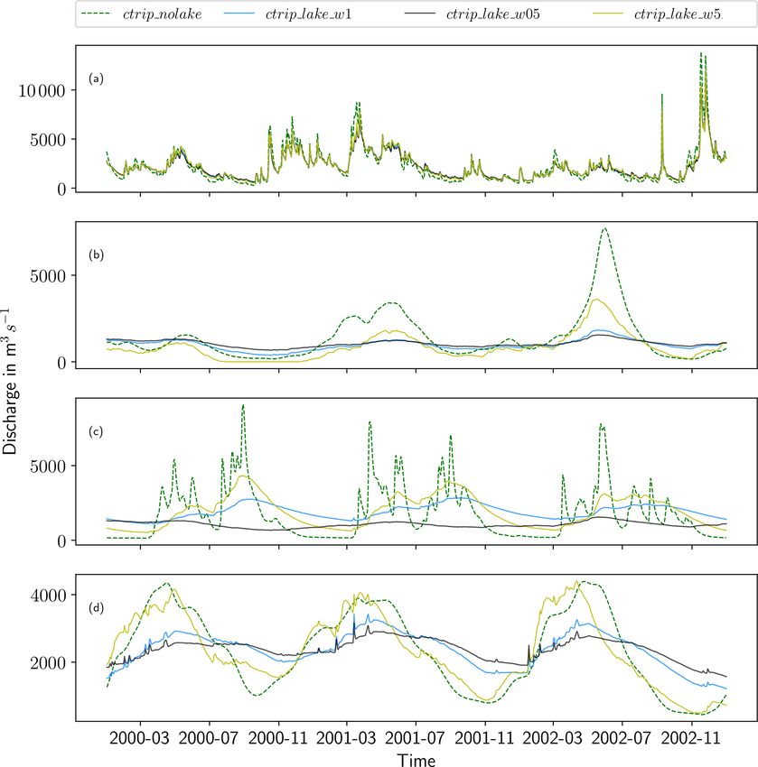
Figure 8. Hydrograph of the simulated river discharge over the period 2000–2002 for the different CTRIP-MLake configurations: (a) Rhône,
(b) Angara, (c) White Nile and (d) Neva.
ysis products (https://www.ecmwf.int/en/forecasts/datasets/ of the model, in order to retrieve streamflows and lake levels
reanalysis-datasets/era-interim, last access: 4 March 2021) compared to the observations. In the following part of the
over the period 1979–2014. Precipitation is adjusted using results, particular attention has been paid to the model’s sen-
the monthly observations from the Multi-Source Weighted- sitivity to the lake outlet width, which is the only adjustable
Ensemble Precipitation (MSWEP, Beck et al., 2017) dataset. parameter.
Decharme et al. (2019) showed the better performance of the
model using E2O forcings compared to PGF forcings, in par- 5.1 Impact of lakes on the ISBA-CTRIP simulations
ticular in terms of river discharge scores, which was mainly
due to higher precipitation rates. The runoff estimations for A benchmark study to evaluate the influence of the new
the Angara, White Nile and Neva watersheds used in the lake module on CTRIP-simulated streamflows was first per-
current study therefore come from the multi-layer diffusive formed consisting in four simulations which are summa-
ISBA forced by the ERA-Interim E2O forcings. rized in Table 4. Due to the model sensitivity to the val-
ues of the weir height, a few years of model spin-up are re-
quired to reach a steady state (the length of the spin-up de-
5 Results pends upon the lake size). This adjustment period is not in-
cluded in the evaluation. The evaluation period ranges from
This study follows a two-step evaluation by first assessing 1 January 1983 to 31 December 2013. The comparison of
the influence of lakes on the CTRIP streamflows simulation the model simulations over the period 2000–2003 is shown
and then the influence of the lake module on the performance in Fig. 8). A general reduction of river discharge variabil-
Geosci. Model Dev., 14, 1309–1344, 2021 https://doi.org/10.5194/gmd-14-1309-2021You can also read