Partitioning the Galactic Halo with Gaussian Mixture Models - arXiv.org
←
→
Page content transcription
If your browser does not render page correctly, please read the page content below
Research in Astronomy and Astrophysics manuscript no.
                                              (LATEX: ms2020-0400.tex; printed on January 8, 2021; 2:35)

                                              Partitioning the Galactic Halo with Gaussian Mixture Models
arXiv:2101.01360v2 [astro-ph.GA] 7 Jan 2021

                                              Xilong Liang1,2 , Yuqin Chen2,1 , Jingkun Zhao2,1 and Gang Zhao2,1

                                              1
                                                  School of Astronomy and Space Science, University of Chinese Academy of Sciences, Beijing 100049,
                                                  China
                                              2
                                                  CAS Key Laboratory of Optical Astronomy, National Astronomical Observatories, Chinese Academy of
                                                  Sciences,Beijing 100101, China; cyq@bao.ac.cn

                                              Received 20xx month day; accepted 20xx month day

                                                      Abstract The Galactic halo is supposed to form from merging with nearby dwarf galaxies.
                                                      In order to probe different components of the Galactic halo, we have applied the Gaussian
                                                      Mixture Models method to a selected sample of metal poor stars with [Fe/H] < −0.7 dex in
                                                      the APOGEE DR16 catalogue based on four-parameters, metallicity, [Mg/Fe] ratio and spa-
                                                      tial velocity (VR , Vφ ). Nine groups are identified with four from the halo (group 1, 3, 4 and
                                                      5), one from the thick disk (group 6), one from the thin disk (group 8) and one from dwarf
                                                      galaxies (group 7) by analyzing their distributions in the ([M/H], [Mg/Fe]), (VR , Vφ ), (Zmax,
                                                      eccentricity), (Energy, Lz) and ([Mg/Mn], [Al/Fe]) coordinates. The rest two groups are re-
                                                      spectively caused by observational effect (group 9) and the cross section component (group
                                                      2) between the thin disk and the thick disk. It is found that in the extremely outer accreted
                                                      halo (group 1), stars born in the Milky Way can not be distinguished from those accreted from
                                                      other galaxies either chemically or kinematically. In the intermediate metallicity of −1.6 <
                                                      [Fe/H] < −0.7 dex, the accreted halo mainly composed of the Gaia-Enceladus-Sausage sub-
                                                      structure (group 5), which can be easily distinguished from group 4 (the in-situ halo group) in
                                                      both chemical and kinematic space. Some stars of group 4 may come from the disk and some
                                                      disk stars can be scattered to high orbits by resonant effects as shown in the Zmax versus
                                                      Energy coordinate. We also displayed the spatial distribution of main components of the halo
                                                      and the ratio of accreted components do not show clear relation to Galactic radius.

                                                      Key words: Galaxy abundances, Galaxy kinematics, Galaxy structure

                                              1 INTRODUCTION

                                              According to the Λ cold dark matter scenario, the halos of large galaxies like the Milky Way grow in
                                              size by merging with small dwarf galaxies, leaving behind debris in the form of different groups of stars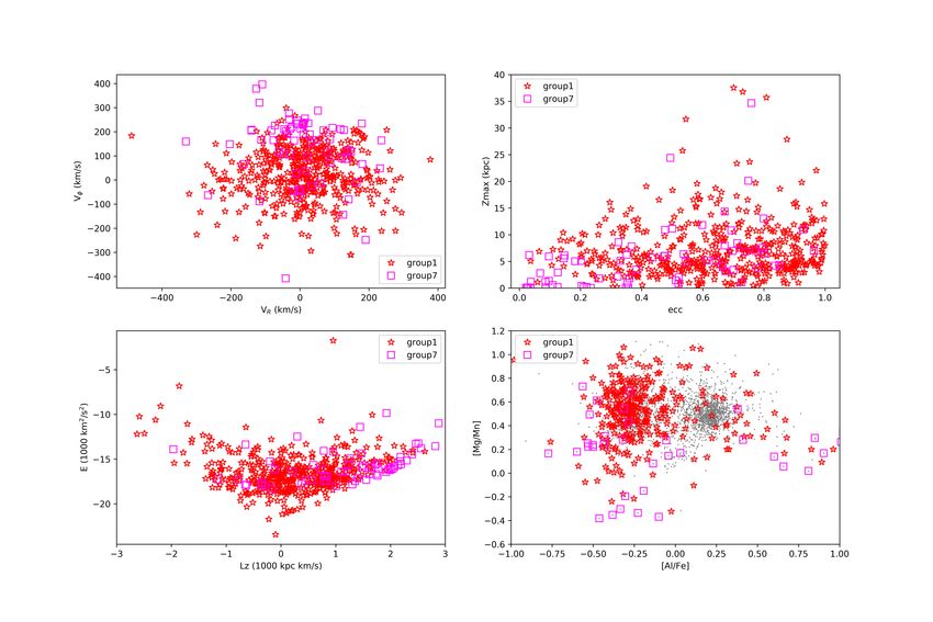
2                                                Liang et al.

spectroscopic surveys (LAMOST (Cui et al. 2012; Zhao et al. 2012); RAVE (Kunder et al. 2017); APOGEE
(Majewski et al. 2017); GALAH (Buder et al. 2018) and so on), the Galactic halo has been analysed both
kinematically and chemically. A number of studies have drawn a consistent picture that a large fraction of
stellar halo was accreted. One recently found velocity structure has been named Gaia-Enceladus-Sausage
(Belokurov 2018; Deason et al 2018; Haywood et al 2018; Helmi et al 2018; Koppelman et al 2018;
Myeong et al 2018c,d; Fattahi 2019), which is speculated to be debris from a massive dwarf galaxy (Gaia
Enceladus) with initial stellar mass about 5 × 10⁸ − 5 × 10⁹ MJ (Belokurov 2018; Helmi et al 2018;
Mackereth et al 2019; Vincenzo et al 2019) and it was supposed to be accreted about 10 Gyr ago (Helmi et
al 2018; Di Matteo et al 2018; Gallart et al 2019). Besides Gaia-Enceladus-Sausage, Myeong et al (2018c)
identified another velocity structure consisting of retrograde, high-energy stars in the halo with metallicity
between −1.9 and −1.3, which is related to ω Centauri by Myeong et al (2018b,c) and is supposed to
be accreted 5 − 8 Gyr ago (Koppelman et al 2019). According to Bekki & Freeman (2003); Majewski
et al (2012), dwarf galaxy ω Centauri is known to be a major source of retrograde halo stars in the inner
Galaxy. Massari et al (2019) argues that Gaia-Enceladus-Sausage is also likely associated with ω Centauri.
A new high-energy, retrograde velocity structure named as term Sequoia is found by Myeong et al (2019).
It is connected with a large globular cluster with very retrograde halo-like motion, FSR-1758 (Barba et al
2019). Based on chemical abundances, Matsuno et al (2019) suggested that this retrograde component is
dominated by an accreted dwarf galaxy, which has a longer star formation timescale and is less massive
than Gaia-Enceladus-Sausage. In summary, Koppelman et al (2019) suggested that the retrograde halo
contains a mixture of debris from objects like Gaia-Enceladus-Sausage, Sequoia, Thamnos and even the
chemically defined thick disc. Based on chemical abundances, Nissen et al (2010) divided the halo into
high α population and low α population and they proposed that the low α population is accreted from
nearby galaxies. Based on SDSS data, Carollo et al. (2007); Carollo et al (2010) classified the halo into the
inner halo with metal rich stars on mildly eccentric orbits and the outer accreted halo with metal poor stars
on more eccentric orbits. From APOGEE DR12, Hayes et al (2018) found that the low [Mg/Fe] population
has a large velocity dispersion with very little or no net rotation. Haywood et al (2018) suggested that
the high α stars thought to belong to an in situ formed halo population may in fact be the low rotational
velocity tail of the old Galactic disk heated by the last significant merger of a dwarf galaxy. Di Matteo et
al (2019) also claimed that about half of the kinematically defined halo within a few kilo parsec from the
Sun is composed of thick disc stars, since the accretion process could lead to the last significant heating
of the thick disk stars into the halo. With [M/H], [Mg/Fe] and distances from APOGEE data release 14,
Chen et al (2019) indicates a three section halo, the inner in situ halo with |Z| less than about 8 − 10
kpc, the intermediately outer dual-mode halo at |Z| between about 10 kpc and 30 kpc, and the extremely
outer accreted halo with |Z| larger than 30 kpc. Carollo & Chiba (2020) found the inner stellar halo is also
comprised of many different components. In a word, the Galactic halo has a complicate history and further
works are desired to unravel its assembling processes.

    This paper aims to partition the Galactic halo by identifying different components in the chemical and
kinematic space. As shown in Nissen et al (2010) and Haywood et al (2018), in the intermediate metallicity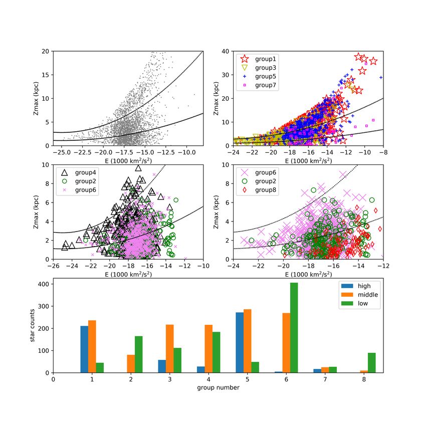
Halo groups                                               3

versus [Mg/Fe] coordinate because there is a clear gap between low [Mg/Fe] and high [Mg/Fe] stars. Those
two populations also have distinguished kinematic properties in the Toomre diagram (Nissen et al 2010),
the VR -Vφ diagram (Haywood et al 2018) and eccentricity distributions (Mackereth et al 2019). Note
that, the separation between the accreted halo and the in-situ halo is not found in the chemical space of
[M/H] versus [Mg/Fe] in the low metallicity range of −2.6 < [Fe/H] < −1.6 dex in the APOGEE data. It
would be of interest to investigate whether the kinematic imprints of the accreted halo can be picked out
for this low metallicity range by using a grouping method that simultaneously takes into account chemical
and kinematic properties. Finally, after groups are selected, studying similarities and differences among
different groups by various combinations of orbital and energy parameters provide new insights on the
complicate assembling history of the Galaxy.

2 DATA AND THE PARTITION METHOD

The sample stars are selected from the APOGEE DR16 dataset (Abolfathi et al. 2018) with parallaxes
and proper motions taken from Gaia DR2 (Gaia Collaboration 2018). We have removed stars with
ASCAPFLAG or STARFLAG warnings and stars with −9999 values of log g, Teff , [Fe/H] and [Mg/Fe].
We chose to use the Bailer-Jones distance GAIA R EST (Bailer-Jones et al. 2018) and removed stars with
(GAIA R HI−GAIA R LO)
          2           /GAIA           R EST > 0.2. After these cuts, there are 165 332 stars left. Then, we
calculated three dimensional velocity components in galactocentric cylindrical coordinate with radial veloc-
ities from APOGEE DR16. Python package astropy has been used to transform observed quantities in ICRS
coordinate into galactocentric cylindrical coordinate. The Sun is placed at height z = 0.014 kpc, galactic
radius R = 8.2 kpc with circular speed Vc = 233.1 km s−1 (McMillan 2011). The peculiar velocity of
the Sun relative to the local standard of rest is taken as (UJ , VJ , WJ ) = (11.1, 12.24, 7.25) km s−1 from
Schönrich (2010). Since we want to analyse main components of the halo in the field, we removed those
stars with PROGRAMNAMEs in the APOGEE DR16 catalogue associated with globular clusters, bulge,
young stellar object, RR Lyrae stars, exoplanets, the Magellanic cloud or open clusters. Moreover, stars with
PROGRAMNAME related to stellar streams and apparently clumped as a small group in the velocity coor-
dinate have been removed. After those observationally clumped stars removed, there are 77 549 stars left.
Stars with [Fe/H] > −0.7 dex mainly belong to disk (Haywood 2013; Bensby et al. 2014; Recio-Blanco et
al. 2014; Hawkins et al. 2015), and we think it is not suitable for our method to decompose halo from those
stars. There are still some stars with [Fe/H] < −0.7 dex belong to the disk, but it is acceptable and we will
keep in mind in later analysis. Finally, with metallicity cut, there are 3067 stars left in our sample. GalPot
(McMillan 2017) has been used to calculate orbital parameters such as energy E, angular momentum L,
maximum height Z of orbit Zmax, guiding radius RG and eccentricity ecc. Eccentricities are computed as
        Rapo −Rper
ecc =   Rapo +Rper   in which Rapo and Rper are respectively the orbital apocenter and pericenter. The Galaxy
potential chosen to calculate these values is the default potential called ”PJM17 best.Tpot” supplied by
GalPot.
   R package Mclust (Scrucca et al. 2016) from RR Core Team (2020) has been used for the model-based
clustering, which allows modelling of data as a Gaussian finite mixture with different covariance structures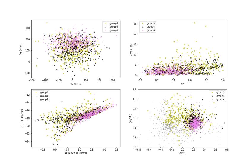
4                                                Liang et al.

                       Fig. 1: BIC and ICL distribute with numbers of components.

ciated with a group or cluster. The Gaussian mixture model assumes a multivariate distribution for each
component and these components are assumed to have ellipsoidal distributions in parameter coordinates
(McLachlan and Peel 2000; Frühwirth-Schnatter 2019). The number of mixing components and the co-
variance parameterization are usually selected using the Bayesian Information Criterion (BIC) (Schwartz
1978; Fraley 1998), which puts its first priority on approximating the density rather than the number of
groups. To solve this problem, Biernacki et al (2000) put forward the integrated complete-data likelihood
(ICL) criterion, which penalises the BIC through an entropy term by measuring overlapping area to obtain
good performance in selecting the number of clusters. When we apply the Gaussian mixture model method
to our sample, both BIC criterion and ICL criterion suggest nine mixing components (groups). Figure 1
shows BIC and ICL values distribute with numbers of components. The BIC criterion suggests nine groups,
while it represents a local maximum for ICL criterion. The real maximum of ICL criterion is at four, and
the four components are the canonical thin disk, the thick disc, the in-situ born halo and the accreted halo.
We choose nine groups because we attempt to study components of the galactic halo rather than main
components of the galaxy.
    Parameters of Gaussian mixture models are obtained via the EM algorithm (Dempster et al. 1977;
McLachlan and Peel 2004). The EM algorithm is a widely used algorithm which has reliable global con-
vergence under fairly general conditions. However, the likelihood surface in mixture models tends to have
multiple modes, and thus initialisation of EM is necessary to produce sensible results when started from
reasonable starting values (Wu 1983). In the R-Mclust package, the EM algorithm is initialised using the
partitions obtained from model-based hierarchical agglomerative clustering (MBHAC). It obtains hierarchi-
cal clusters by recursively merging the two clusters with smallest decrease in the classification likelihood
for Gaussian mixture model (Banfield and Raftery 1993; Fraley & Raftery 1998). The underlying prob-
Halo groups 5
Table 1: Parameters of 9 groups.
number [Fe/H] [Mg/Fe] VR Vφ counts Vz Zmax RG ecc E Lz comments
km s−1 km s−1 km s−1 kpc kpc km2 s−2 kpc km s−1
1 −1.69 0.29 10.6 27.7 492 6.0 7.53 3.12 0.65 −16898 217 extremely outer accreted halo
2 −0.80 0.25 14.4 180.1 247 2.15 2.13 7.16 0.26 −16563 1684 cross section
3 −1.15 0.31 1.2 104.0 387 −2.03 4.09 3.92 0.54 −17575 847 canonical halo
4 −0.86 0.31 12.4 118.6 428 −0.16 2.86 4.25 0.52 −17649 934 inner in-situ halo
5 −1.09 0.18 −16.9 23.9 607 2.33 8.20 2.13 0.80 −16094 192 accreted halo
6 −0.75 0.31 −0.1 170.8 680 −4.02 2.24 5.86 0.35 −17086 1371 the thick disk
7 −1.45 0.12 24.4 85.9 69 −20.9 6.85 6.53 0.44 −15381 1189 accreted stars
8 −0.72 0.14 −7.0 223.6 100 −3.39 1.63 10.04 0.13 −15154 2368 the thin disk
9 −1.41 0.17 −23.6 157.3 57 −124.3 9.66 5.09 0.38 −15372 1180 observational effect
applied to coarse data as ours, the MBHAC approach has a problem that the final EM solution depends
on the ordering of the variables. This problem has been solved by using the method presented by Scrucca
and Raftery (2015). Before applying the MBHAC at the initialisation step, the data is projected through
a suitable transformation, which enhances separation among groups or clusters. Once a reasonable hierar-
chical partition is obtained, the EM algorithm is run using the data on the original scale. Via this approach,
different orders of variables won’t affect fitted model any more and the result becomes stable.
3 RESULTS
We applied the Gaussian mixture models to our data sample in a joint space of [Fe/H], [Mg/Fe], VR and
Vφ and got nine groups. Table 1 lists mean values of nine gaussian models fitted by the R-Mclust package.
The first column is the number of groups given by R-Mclust package(Keribin 2000; McLachlan 1987;
McLachlan and Rathnayake 2014), while the sixth column lists star counts in each group. Table A.1 in the
Appendix lists covariance matrixes of fitted gaussian distribution of each group with variables ordered as
([Fe/H], [Mg/Fe], VR , Vφ ). The rest columns of table 1 list mean values of some kinematical and dynamical
parameters after groups were obtained. With more parameters, there would be more smaller substructures
with fewer stars in each group. Since we focus on the main components of the halo rather than small
substructures, we chose to use these four parameters that can best describe the main components in our
sample.
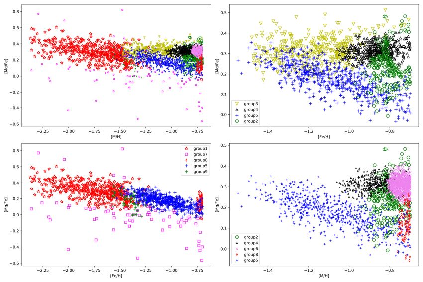
Figure 2 shows nine groups in the [Mg/Fe] versus [Fe/H] coordinate fitted by Gaussian mixture model.
The top left panel shows overall distributions of nine groups, while other three panels show relative posi-
tions of adjacent groups more clearly. Although Gaussian distribution is not a good model to describe the
chemical plane, because stars counts of groups monotonously increase with the increase of metallicity in
our sample, it is enough to pick out main components in the sample. Group 3, group 4 and group 6 have sim-
ilar mean magnesium abundance values around 0.31 and they form the horizontal high-[Mg/Fe] sequence.
Group 5, group 8 and group 9 in the lower panel have relatively lower mean magnesium abundance, and
Group 7 has even lower [Mg/Fe] ratios. Group 5 takes up the position of canonical accreted halo in the6 Liang et al. Fig. 2: The top left panel shows nine groups in the [Mg/Fe] versus [M/H] coordinates, while other three subplots show relatively positions of adjacent groups more clearly. Sect. 3.1). Group 8 lies at the metal rich end of group 5 and the metal poor end of the thin disk, while group 6 lies at the metal poor end of the thick disk. Group 1 has an increasing [Mg/Fe] with decreasing metallicity and thus we classify it as the extension of the low-[Mg/Fe] sequence. 3.1 Group 9 Figure 3 shows distributions of group 9 (green plus) in the (x, z) and (Lz, E) coordinates and background grey dots represent the total sample. Grey dots in the upper panel of figure 3 shows distributions of our total sample in the x-z positional space. As shown in the upper panel, group 9 has a almost continuous linear distribution in the x-z plane and it is the last group ordered by statistical significance. Its position in the E versus Lz coordinate is very close to Helmi streams (Helmi et al 1999; Koppelman et al 2018, 2019; Naidu et al. 2020; Helmi 2020) and we conjecture their observations are related to the Helmi streams. The detection of the Helmi stream is interesting, which may indicate that this method is powerful enough to pick out even small groups with related chemical and kinematic properties. Though we have tried to exclude stars from obvious moving groups which apparently clumped in velocity coordinate when selected the sample, there are still some left in our sample. In a word, we think group 9 is caused by observational effect and do not discuss about it later. 3.2 Group 3, group 4 and group 6 The high-[Mg/Fe] sequence is separated into threes groups (3,4,6) in our sample by the Gaussian mixture
Halo groups                                                7

Fig. 3: Group 9 (green plus) in the (x, z) and (Lz, E) coordinates. Those blue plus are the small over-density
in top left of group 5 in figure 5. Those background grey dots represent the total sample.

stars. Group 4 and group 3 have very similar distribution ranges and similar scatters in the Vφ versus VR
coordinate, which means kinematically they can not distinguish from each other. The top right panel of
figure 4 shows Zmax versus eccentricity distribution of group 3, group 4 and group 6. Group 3 can reach
higher region than group 4 and group 6. Most stars of group 6 have roundish orbits and can not run out
8                                                Liang et al.

Fig. 4: Group 3, group 4 and group 6 in (VR , Vφ ), (ecc, Zmax), (Lz, E) and ([Al/Fe], [Mg/Mn]) coordinates
and background grey dots represent our total sample.

dual-mode halo or the canonical halo (Hawkins et al. 2015). In the bottom left subplot, group 4 have almost
similar distribution range as group 3, except its energy is slightly smaller than that of group 3 on the whole.
To cleanly distinguish halo component and disk component, the last panel shows those three groups in the
[Mg/Mn] versus [Al/Fe] coordinate (Hawkins et al. 2015). In the last panel group 4 and group 6 both mainly
clumps in the disk region and can not distinguish from each other, While distribution of group 3 reaches to
the disk region. Group 4 is tightly related to the disk region that it seems like smoothly extend out of the
disk region in all parameter spaces. Since group 4 represents the inner in-situ halo in kinematics but has
strong connection to the thick disk in chemistry, we suggest that part of it comes from disk heating (Quinn
et al. 1993; Di Matteo et al 2019; Grand et al. 2020; Yu et al. 2020).

3.3 Group 5 and group 8

In figure 5, group 8 locates at the metal rich end of group 5 and the metal poor end of the thin disk. However,
their distributions in kinematical and dynamical coordinates clearly separate from each other. With high Vφ
speed, low eccentricity and small Zmax, group 8 represents the thin disk component in our sample. Group 5
represents the canonical accreted halo component (Hawkins et al. 2015) according to its position in figure 2.
Group 5 is mainly composed of Gaia-Enceladus-Sausage, but includes more than just it. Since our sample
stars are within z ≈10 kpc, we conformed that Gaia-Enceladus-Sausage is the dominant component of
the halo (Naidu et al. 2020) in this spatial range. There is a megascopic group of stars clumped in the top
left region of group 5 in the Vφ versus VR coordinate. As is shown in figure 3, They have a continuous
Halo groups                                                9

Fig. 5: Group 5 and group 8 in (VR , Vφ ), (ecc, Zmax), (Lz, E) and ([Al/Fe], [Mg/Mn]) coordinates and
background grey dots represent our total sample.

abundances of these stars is very close to group 9 (the Helmi stream) too. But they have different VR
coordinates and larger eccentricity distributions than stars in group 9. We think they may be related to the
Helmi stream and it is normal that some stars from the Helmi stream or other streams are classified into the
accreted halo (group 5). Group 5 not only cleanly separates from the thin disk in kinematical and dynamical
coordinates, but also has different distribution from the thin disk in the [Mg/Mn] versus [Al/Fe] coordinate.
Unlike group 3 in figure 4, chemical distribution of group 5 is apparently separated from the disk region with
only few stars scattering in the disk region. Comparing our bottom left panel with selection criteria in Naidu
et al. (2020), there are many dynamical substructures in the accreted halo such as Gaia-Enceladus-Sausage,
Wukong, Helmi streams and Aleph.

3.4 Group 1 and group 7

Figure 6 shows group 1 and group 7 in kinematic and dynamical coordinates. Group 1 represents the metal
poorest part of the halo while group 7 is composed of stars with poorest magnesium abundances in our
sample. They both have large ranges of velocity distributions and spatial distributions. In the E versus Lz
coordinate, group 1 overlaps with parts of some dynamical substructures such as Gaia-Enceladus-Sausage,
Wukong, Arjuna, Sequoia, I’itoi, Thamnos and Aleph (Naidu et al. 2020). Group 1 has large scatters for
both kinematics and chemical abundances distributions. And in all those subplots of figure 6, group 1 shows
smooth distributions. Within group 1, stars born in the Milky Way can not be distinguished from those
accreted from other galaxies either chemically or kinematically. The bottom right panel of figure 6 shows
10                                               Liang et al.

Fig. 6: Group 1 and group 7 in (VR , Vφ ), (ecc, Zmax), (Lz, E) and ([Al/Fe], [Mg/Mn]) coordinates and
background grey dots represent our total sample.

total sample. Main parts of these two groups clearly distribute away from the disk region and group 7 seems
distribute slightly father away from the disk than group 1. Group 7 has even poorer metallicity and lower
Magnesium abundance than group 5, the accreted halo. Based on these properties, we suggest that group 1
represents the extremely outer accreted halo, while group 7 might be related to dwarf galaxies due to lower
[Mg/Fe] than the accreted halo, typical for dwarf galaxies.

3.5 Group 2

In figure 2, group 2 distributes over both high-[Mg/Fe] branch and low-[Mg/Fe] branch and it connects the
thin disk, the thick disk, the in-situ halo and the accreted halo. The kinematic and dynamical distributions
of group 2 in figure 7 behave like a disk component. Most stars of group 2 have not very large eccentricity
and highest distances away from the Galactic middle plane and thus they are mainly born in the disk region.
In the last panel, [Mg/Mn] versus [Al/Fe] distribution of group 2 mainly locates at disk region with few
low [Al/Fe] or high [Mg/Mn] stars permeating into halo region. As compared with group 8, group 2 has the
main component of the thick disk with higher [Al/Fe] or high [Mg/Mn] ratios but it has a tail extending to
lower values, overlapping with the thin-disk region. Thus, group 2 represents the cross section of thin disk
and the thick disk and may contains some stars from accreted halo. Usually the cross section is not very
obvious, but most stars of group 2 distribute close to the Sun in spatial coordinates. The observational effect
Halo groups                                                 11

Fig. 7: Group 2 in (VR , Vφ ), (ecc, Zmax), (Lz, E) and ([Al/Fe], [Mg/Mn]) coordinates and background grey
dots represent our total sample.

3.6 Discussion

Figure 8 shows those eight groups in Zmax versus E coordinates. The top left subplot shows the distribution
of our total sample, and it apparently distributes into three blocks. Two black dotted curves are subjectively
drawn to show boundaries between those three blocks caused by transitions from one orbital family to
another (Moreno et al. 2015; Haywood et al 2018; Amarante et al. 2020). The locations of these gaps
marked by black dotted curves are determined by the adopted potential and cannot be used to learn about the
physical origins of the stars (Moreno et al. 2015; Amarante et al. 2020). Nonetheless, it is still interesting to
see some disk stars being scattered to high orbits by resonant effects. The bottom subplot of figure 8 shows
stars orbital distribution of each group in high, middle and low orbital families. We notice that the accreted
halo groups, group 1 and group 5 has similar distributions with comparable fraction between the high and
middle sections and little contribution from the low section. Group 2 and group 6 have main contribution
from the low section but significant fraction from the middle section, which is consistent with the thick
disk population. Group 4 shows a larger fraction of the middle section than the low section, similar as the
in-situ halo of group 3, and thus indicates an evidence for disk heating. The star number in group 7 is too
small to draw conclusion. Group 8 has main distribution in the low section in consistent with the thin disk
population.
   Figure 9 shows spatial distributions of our nine groups in (R, z) coordinates. While bottom two stacked
bar charts show distributions of percentages each group take up in small bins taken along R and z direction
with size equal to 0.5 kpc. Group 1 and group 5 have the largest spatial distributions while group 6 and
12                                               Liang et al.

                                    Fig. 8: E versus Zmax distributions.

and kinematical parameters. The spatial distribution of our sample is restricted by observational effect that
most stars distribute around the sun as shown in top four panels. But percentage distributions reveal some
tendencies. In the bottom left panel, the large R end is mainly composed of group 8 (the thin disk), group 7
(accreted stars), group 5 (accreted halo), group 1 (extremely outer accreted halo) and group 2 (cross section
of disks). For group 8, only the bin at 8 kpc contains more than 10 stars, but it still needs explanation why
group 8 takes up about twenty percent of our total sample at large R region. As is shown in the bottom left
panel, group 4 (inner in-situ halo) take up very small percentages in bins around the large R end relative to
other regions, while group 2 and group 8 take up relatively larger percentages at this region. As is known,
there is radial abundance gradients of the disk (Shaver et al. 1983; Liang et al. 2019) and at large radius,
the flare and warp of the disk make it more easily been observed. Considering our sample is selected by
metallicity cut, it is reasonable the thin disk component takes up more percentage at large R region. It is
also possible there are several thick disk stars or accreted stars or accreted halo stars mixed in group 8.
For radius larger than the Galactic center regions (around 3 kpc), group 1 takes up similar percentages
Halo groups 13 Fig. 9: Spatial distributions of each group. Bins of 0.5 kpc have been taken along R and z direction to obtain star counts in the bottom two panels. radius and we think group 8 might contain several stars from dwarf galaxies too. In the last panel, group 6 (the thick disk component) dominates the Galactic mid-plane region while group 1 and group 5 dominate regions far away from the Galactic mid-plane. Group 4 distributes around the Galactic mid-plane while group 3 (canonical halo) does not show clear preference for z distribution. The inner in-situ halo (group 4)
14                                              Liang et al.

4 CONCLUSION

A sample of stars with reliable stellar parameters in the ranges of [Fe/H] < −0.7 dex, −0.5 < [Mg/Fe] < 0.6
dex, Zmax < 90 kpc, E < 0 km2 s−2 and | Lz |< 5000 kpc km s−1 is selected from the APOGEE DR16
catalogue. Gaussian mixture model has been applied to this sample by using both chemical abundances
parameters of [Mg/Fe] and [M/H] and two velocity components of VR , Vφ . Nine groups are detected, in
which group 9 is part of the Helmi stream caused by observational effect. We analysed distributions of
each group on the [M/H] versus [Mg/Fe], VR versus Vφ , the Zmax versus eccentricity, Energy versus Lz
and [Mg/Mn] versus [Al/Fe] diagrams in order to trace their origins. Group 1 represent the extremely outer
accreted halo, while group 7 comes from dwarf galaxies. Comparing the position of group 1 in the Lz versus
E diagram with the streams of Koppelman et al (2019) indicate that group 1 includes many accreted stars
from Sequoia, Thamno 1 and Thamno 2 substructures as well as many local born halo stars. Group 5 is
the accreted halo dominated by the well known Gaia Enceladus/Sausage, which is clearly separated from
the in-situ halo of group 3 in both chemical ([Mg/Fe] and [Al/Fe]) and kinematic spaces (VR versus Vφ
and the Lz versus E diagrams). We may see a signature of disk heating in group 4, part of which has a
halo-kinematics in the VR versus Vφ diagram but disk-chemistry in the [Mg/Mn] versus [Al/Fe] diagram.
Group 6 and group 8 show typical properties for the classical thick disk and the thin disk respectively,
while group 2 may consists mainly thick disk stars with a small fraction of thin disk stars. In the E versus
Zmax diagram, three sections are found and the relative fractions provide further support on the similar
origin of group 1 and group 5 from the accreted halo, of group 2 and group 6 from the thick disk, as well
as the signature of disk heating for group 4 (as compared with the in-situ halo of group 3). These results
indicate that the Galactic halo has complicated assembly history and it not only interacts but also strongly
mixed with other components of the Galaxy and satellite dwarf galaxies. In addition, dynamical evolution
and chemical evolution of the Galaxy are entangled, and these factors should be considered together in the
simulation works in the future.

Acknowledgements We thank the reviewer for his/her constructive suggestions. This study is sup-
ported by the National Natural Science Foundation of China under grants No. 11988101, 11625313,
11973048, 11927804, 11890694 and National Key R&D Program of China No. 2019YFA0405502 and
the Fundamental Research Funds for the Central Universities under grants No. 292020001734 (E0E48956).
     Funding for the Sloan Digital Sky Survey IV has been provided by the Alfred P. Sloan Foundation,
the U.S. Department of Energy Office of Science, and the Participating Institutions. SDSS-IV acknowl-
edges support and resources from the Center for High-Performance Computing at the University of Utah.
The SDSS web site is www.sdss.org. SDSS-IV is managed by the Astrophysical Research Consortium
for the Participating Institutions of the SDSS Collaboration including the Brazilian Participation Group,
the Carnegie Institution for Science, Carnegie Mellon University, the Chilean Participation Group, the
French Participation Group, Harvard-Smithsonian Center for Astrophysics, Instituto de Astrofı́sica de
Canarias, The Johns Hopkins University, Kavli Institute for the Physics and Mathematics of the Universe
(IPMU) / University of Tokyo, the Korean Participation Group, Lawrence Berkeley National Laboratory,
Leibniz Institut für Astrophysik Potsdam (AIP), Max-Planck-Institut für Astronomie (MPIA Heidelberg),
Halo groups 15
(MPE), National Astronomical Observatories of China, New Mexico State University, New York University,
University of Notre Dame, Observatário Nacional / MCTI, The Ohio State University, Pennsylvania
State University, Shanghai Astronomical Observatory, United Kingdom Participation Group, Universidad
Nacional Autónoma de México, University of Arizona, University of Colorado Boulder, University of
Oxford, University of Portsmouth, University of Utah, University of Virginia, University of Washington,
University of Wisconsin, Vanderbilt University, and Yale University.
This work has made use of data from the European Space Agency (ESA) mission Gaia
(https://www.cosmos.esa.int/gaia), processed by the Gaia Data Processing and Analysis Consortium
(DPAC, https://www.cosmos.esa.int/web/gaia/dpac/consortium). Funding for the DPAC has been provided
by national institutions, in particular, the institutions participating in the Gaia Multilateral Agreement.
Appendix A: GAUSSIAN FINITE MIXTURE MODEL
Let x = (x1 , x2 , ..., xi , ..., xn ) be a sample of n independent identically distributed observations from a
probability density function through a finite mixture model of g Gaussian components, which takes the
following form
g
X
f (xi , Ψ) = πi φ(xi ; µi , Σi )
i=1
Where Ψ = (π1 , ..., πg − 1, ξ T )T are parameters of the mixture model. ξ contains the elements of
the component mean µi and covariance matrices Σi , while πi is the mixing weight or probability of each
component. For our case, each observation is composed of four variables ordered as ([Fe/H], [Mg/Fe], VR ,
Vφ ). Mean values of nine multivariate Gaussian distributions have been listed in table 1, while table A.1
lists covariance matrixes of these nine components.16 Liang et al.
Table A.1: Covariance matrix of fitted gaussian distributions. They are ordered by group numbers with four
used variables for each covariance matrix ordered as ([Fe/H], [Mg/Fe], VR , Vφ ).
0.09349142 -0.01670629 -0.0510382 -5.4292427
-0.01670629 0.01039478 0.3099455 0.7175462
(A.1)
-0.05103820 0.30994546 14693.3 288.5084
-5.42924271 0.71754620 288.508 10116.28
0.0034185456 0.0004206848 0.3631803 -0.7387926
0.0004206848 0.0078440981 1.2687077 -1.2341388
(A.2)
0.3631803393 1.2687077 3059.0287 23.3533386
-0.7387926 -1.23413881 23.3533386 1826.7034
0.03838573 0.003348854 -5.2917447 3.4282508
0.00334885 0.004225013 -0.2554129 -0.4454307
(A.3)
-5.29174471 -0.255413 7421.4537 -587.3283
3.42825076 -0.445430748 -587.3283 6411.704
0.0075656207 0.0005721973 -1.0612834 -2.9071771
0.0005722 0.0011567533 0.1007521 -0.2963813
(A.4)
-1.0612833 0.1007521000 7554.22 221.595
-2.907177 -0.29638133 221.595 5618.139
0.04021166 -0.01154754 1.2517914 -0.4534044
-0.01154754 0.00621082 0.4413265 -0.7344783
(A.5)
1.25179140 0.4413265 27383.1653 -1998.32
-0.45340438 -0.7344783 -1998.32 4412.365
0.00093047 -0.00002497 0.01589945 -0.0076799
-0.00002497 0.001245 0.02610716 0.08878
(A.6)
0.015899 0.02610716 6691.895 313.2556
-0.0076798 0.08878387 313.2556 2258.296
0.18996237 -0.05379311 1.236969 20.72871
-0.05379311 0.06226352 5.277472 -11.82159
(A.7)
1.23696882 5.27747232 10628.428 -3281.21520
20.72870640 -11.82159321 -3281.2 18444.13
0.000314823 0.0001351775 − 0.1034287 0.01897870
0.000135178 0.0059722326 -0.7496104 -0.06235303
(A.8)
-0.10342873 -0.749610434 991.1423 106.8586878
0.0189787 -0.062353027 106.85869 643.55376
0.006454853 -0.00370338 0.01633454 -0.0272713
-0.00370338 0.007584 -0.0640229 0.01518699
(A.9)
0.016334538 -0.0640229 52.2878872 44.091147
-0.02727136 0.015187 44.0911476 73.628824Halo groups 17 References Abolfathi B., Aguado D. S., Aguilar G. et al. 2018, ApJS, 235, 42 Amarante, J. A. S., Smith, M. C., & Boeche, C. 2020, MNRAS, 492, 3816 Antoja, T., Helmi, A., Romero-Gómez M., 2018, Nature, 561, 360 Bailer-Jones, C. A. L., Rybizki, J., Fouesneau, M., Mantelet, G., & Andrae, R. 2018, AJ, 156, 58 J. Banfield and A. E. Raftery. Model-based Gaussian and non-Gaussian clustering. Biometrics, 49: 803–821, 1993. [p291, 304, 314] Barba, R. H., Minniti, D., Geisler, D., et al. 2019, ApJ, 870, L24 Barros, D. A., Pérez-Villegas, A., Lépine, J. R. D., et al 2020, ApJ, 888, 75 Bekki, K., & Freeman, K. C. 2003, MNRAS, 346, L11 Belokurov, V., Erkal, D., Evans, N. W., Koposov, S. E., & Deason, A. J. 2018, MNRAS, 478, 611 Bensby, T., Feltzing, S., & Oey, M. S. 2014, A&A, 562, A71 C. Biernacki, G. Celeux, and G. Govaert, 2000, IEEE Transactions on Pattern Analysis and Machine Intelligence, 22(7), 719 Bressan, A., Marigo, P., Girardi, L., et al. 2012, MNRAS, 427, 127 Buder, S., Asplund, M., Duong, L., et al. 2018, MNRAS, 478, 4513 Carollo, D., Beers, T. C., Lee, Y. S., et al. 2007, Nature, 450, 1020. doi:10.1038/nature06460 Carollo, D., Beers, T. C., Chiba, M., et al. 2010, ApJ, 712, 692 Carollo, D. & Chiba, M. 2020, arXiv:2010.00235 Chen Y Q, Zhao G, Xue X X, et al. 2019, ApJ, 871(2), 216. Cui, X.-Q., Zhao, Y.-H., Chu, Y.-Q., et al. 2012, Research in Astronomy and Astrophysics, 12, 1197 Deason, A. J., Belokurov, V., Koposov, S. E., & Lancaster, L. 2018, ApJ, 862, L1 A. P. Dempster, N. M. Laird, and D. B. Rubin, 1977, Journal of the Royal Statistical Society: Series B (Statistical Methodology), 39(1), 1 Di Matteo, P., Haywood, M., Lehnert, M. D., et al. 2018, A&A, 604, A106 Di Matteo P, Haywood M, Lehnert M D, et al. 2019, A&A, 632, A4 Fattahi, A., Belokurov, V., Deason, A. J., et al. 2019, MNRAS, 484, 4471 Fernández-Alvar E, Fernández-Trincado J G, Moreno E, et al. 2019, MNRAS, 487(1), 1462 Fragkoudi, F., Katz, D., Trick, W., et al. 2019, MNRAS, 488, 3324 C. Fraley. Algorithms for model-based Gaussian hierarchical clustering. SIAM Journal on Scientific Computing, 20(1):270–281, 1998. [p304] C. Fraley and A. E. Raftery, 1998, The Computer Journal, 41(8), 578 S. Frühwirth-Schnatter, Gilles Celeux, Christian P. Robert, Handbook of Mixture Analysis, CRC Press, 2019 Frenk CS, White SDM. 2012. Annalen der Physik 524:507–534 Gaia Collaboration, Brown, A. G. A., Vallenari, A., et al. 2018, A&A, 616, A1 Gallart, C., Bernard, E. J., Brook, C. B., et al. 2019, Nat. Astron., 3, 932 Grand, R. J. J., Kawata, D., Belokurov, V., et al. 2020, MNRAS, 497, 1603 Hawkins, K., Jofré, P., Masseron, T., et al. 2015, MNRAS, 453, 758
18                                                   Liang et al.

Hayes, C. R., Majewski, S. R., Hasselquist, S., et al. 2018, ApJ, 852, 49
Hayes, C. R., Majewski, S. R., Hasselquist, S., et al. 2020, ApJ, 889, 63
Haywood, M. 2013, Memorie della Societa Astronomica Italiana Supplementi, 25, 11
Haywood, M., Di Matteo, P., Lehnert, M. D., et al. 2018, ApJ, 863, 113
Helmi, A., & White, S. D. M. 1999, MNRAS, 307, 495
Helmi, A., Babusiaux, C., Koppelman, H. H., et al. 2018, Nature, 563, 85
Helmi, A. 2020, arXiv e-prints, arXiv:2002.04340
Katz D., Antoja T., Romero-Gómez M., et al., 2018, A&A, 616, A11
C. Keribin. Consistent estimation of the order of mixture models. Sankhyã : The Indian Journal of Statistics,
     Series A (1961–2002), 62(1):49–66, 2000. [p295]
Khanna, S., Sharma, S., Tepper-Garcia, T., et al. 2019, MNRAS, 489, 4962
Koppelman, H. H., Helmi, A., & Veljanoski, J. 2018, ApJ, 860, L11
Koppelman H H, Helmi A, Massari D, et al. 2019, A&A, 631: L9.
Koppelman, H. H., Helmi, A., Massari, D., Roelenga, S., & Bastian, U. 2019b, A&A, 625, A5
Kunder, A., Kordopatis, G., Steinmetz, M., et al. 2017, AJ, 153, 75
Laporte, C. F. P., Minchev, I., Johnston, K. V., et al. 2019, MNRAS, 485, 3134
Li, C.D., Zhao, G., Zhai, M. & Jia, Y.P. 2018, ApJ, 860, 53
Liang, X., Zhao, J., Chen, Y., et al. 2019, ApJ, 887, 193
Mackereth, J. T., Schiavon, R. P., Pfeffer, J., et al. 2019, MNRAS, 482, 3426
Majewski, S. R., Nidever, D. L., Smith, V. V., et al. 2012, ApJ, 747, L37
Majewski, S. R., Schiavon, R. P., Frinchaboy, P. M., et al. 2017, AJ, 154, 94
Massari, D., Koppelman, H. H., & Helmi, A. 2019, A&A, 630, L4
Matsuno T, Aoki W, Suda T. 2019, ApJ, 874(2), L35
McLachlan G. J. 1987, Journal of the Royal Statistical Society: Series C (Applied Statistics), 36(3), 318
McLachlan        G.    J.,   Peel   D.,      2000,     Finite       Mixture   Models.   Wiley,   New    York,
     http://opac.inria.fr/record=b1097397.
McLachlan G J, Peel D., 2004, Finite mixture models, John Wiley & Sons, [p291, 298, 299]
McLachlan G J, Rathnayake S, 2014, Wiley Interdisciplinary Reviews: Data Mining and Knowledge
     Discovery, 4(5), 341
McMillan P. J. 2011, MNRAS, 414, 2446
McMillan, P. J., 2017, MNRAS, 465, 76
Michtchenko, T. A., Barros, D. A., Pérez-Villegas, A., et al. 2019, ApJ, 876, 36
Minchev, I., Quillen, A. C., Williams, M., et al. 2009, MNRAS, 396, L56
Moreno, E., Pichardo, B., & Schuster, W. J. 2015, MNRAS, 451, 705
Myeong G. C., Evans N. W., Belokurov V., Sanders J. L., Koposov S. E. 2018b, MNRAS, 478, 5449
Myeong G. C., Evans N. W., Belokurov V., Sanders J. L., Koposov S. E. 2018c, ApJ, 856, L26
Myeong G. C., Evans N. W., Belokurov V., Sanders J. L., Koposov S. E. 2018d, ApJ, 863, L28
Myeong, G. C., Vasiliev, E., Iorio, G., Evans, N. W., & Belokurov, V. 2019, MNRAS, 488, 1235
Naidu, R. P., Conroy, C., Bonaca, A., et al. 2020, ApJ, 901, 48
Halo groups 19 Nissen, P. E., & Schuster, W. J. 2010, A&A, 511, L10 Quinn, P. J., Hernquist, L., & Fullagar, D. P. 1993, ApJ, 403, 74 Ramos, P., T. Antoja, F. Figueras., 2018, A& A, 619, A72 R Core Team (2020). R: A language and environment for statistical computing. R Foundation for Statistical Computing, Vienna, Austria. URL https://www.R-project.org/. Recio-Blanco, A., de Laverny, P., Kordopatis, G., et al. 2014, A&A, 567, A5 Scrucca L., Fop M., Murphy T. B., and Raftery A. E., 2016, The R Journal, 8(1), 205 Schönrich R., Binney J., Dehnen W., 2010, MNRAS, 403, 1829 G. Schwartz, 1978, The Annals of Statistics, 6(2),461 L. Scrucca and A. E. Raftery, 2015, Advances in Data Analysis and Classification, 4(9), 447 Shaver, P. A., McGee, R. X., Newton, L. M., et al. 1983, MNRAS, 204, 53 Vincenzo, F., Spitoni, E., Calura, F., et al. 2019, MNRAS, 487, 47 C. J. Wu, 1983, The Annals of Statistics, 11(1), 95 Yu, S., Bullock, J. S., Wetzel, A., et al. 2020, MNRAS, 494, 1539 Zhao, G., Zhao, Y.-H., Chu, Y.-Q., et al. 2012, Research in Astronomy and Astrophysics, 12, 723 Zhao, G., Y.-Q., et al. 2021, eprint arXiv, arXiv:2012.01282
You can also read