Alpha and beta diversity patterns of polychaete assemblages across the nodule province of the eastern Clarion-Clipperton Fracture Zone equatorial ...

Page created by Rafael Nelson
 
CONTINUE READING
Alpha and beta diversity patterns of polychaete assemblages across the nodule province of the eastern Clarion-Clipperton Fracture Zone equatorial ...
Biogeosciences, 17, 865–886, 2020
https://doi.org/10.5194/bg-17-865-2020
© Author(s) 2020. This work is distributed under
the Creative Commons Attribution 4.0 License.

Alpha and beta diversity patterns of polychaete assemblages across
the nodule province of the eastern Clarion-Clipperton Fracture
Zone (equatorial Pacific)
Paulo Bonifácio1 , Pedro Martínez Arbizu2 , and Lénaïck Menot1
1 Ifremer,
         Centre Bretagne, REM EEP, Laboratoire Environnement Profond, ZI de la Pointe du Diable,
CS 10070, 29280 Plouzané, France
2 German Centre for Marine Biodiversity Research (DZMB), Senckenberg am Meer, 26382 Wilhelmshaven, Germany

Correspondence: Lénaïck Menot (lenaick.menot@ifremer.fr) and Paulo Bonifácio (bonif@me.com)

Received: 28 June 2019 – Discussion started: 4 July 2019
Revised: 16 January 2020 – Accepted: 21 January 2020 – Published: 20 February 2020

Abstract. In the abyssal equatorial Pacific Ocean, most            eas and 49 % were singletons. The patterns in community
of the seafloor of the Clarion-Clipperton Fracture Zone            structure and composition were mainly attributed to varia-
(CCFZ), a 6 million km2 polymetallic nodule province, has          tions in organic carbon fluxes to the seafloor at the regional
been preempted for future mining. In light of the large envi-      scale and nodule density at the local scale, thus supporting
ronmental footprint that mining would leave and given the di-      the main assumptions underlying the design of the APEIs.
versity and the vulnerability of the abyssal fauna, the Interna-   However, the APEI no. 3, which is located in an oligotrophic
tional Seabed Authority has implemented a regional manage-         province and separated from the CCFZ by the Clarion Frac-
ment plan that includes the creation of nine Areas of Partic-      ture Zone, showed the lowest densities, lowest diversity, and
ular Environmental Interest (APEIs) located at the periphery       a very low and distant independent similarity in community
of the CCFZ. The scientific principles for the design of the       composition compared to the contract areas, thus question-
APEIs were based on the best – albeit very limited – knowl-        ing the representativeness and the appropriateness of APEI
edge of the area. The fauna and habitats in the APEIs are un-      no. 3 to meet its purpose of diversity preservation. Among
known, as are species’ ranges and the extent of biodiversity       the four exploration contracts, which belong to a mesotrophic
across the CCFZ.                                                   province, the distance decay of similarity provided a species
   As part of the Joint Programming Initiative Healthy and         turnover of 0.04 species km−1 , an average species range of
Productive Seas and Oceans (JPI Oceans) pilot action “Eco-         25 km and an extrapolated richness of up to 240 000 poly-
logical aspects of deep-sea mining”, the SO239 cruise pro-         chaete species in the CCFZ. By contrast, nonparametric esti-
vided data to improve species inventories, determine species       mators of diversity predict a regional richness of up to 498
ranges, identify the drivers of beta diversity patterns and as-    species. Both estimates are biased by the high frequency
sess the representativeness of an APEI. Four exploration con-      of singletons in the dataset, which likely result from under-
tract areas and an APEI (APEI no. 3) were sampled along a          sampling and merely reflect our level of uncertainty. The as-
gradient of sea surface primary productivity that spanned a        sessment of potential risks and scales of biodiversity loss due
distance of 1440 km in the eastern CCFZ. Between three and         to nodule mining thus requires an appropriate inventory of
eight quantitative box cores (0.25 m2 ; 0–10 cm) were sam-         species richness in the CCFZ.
pled in each study area, resulting in a large collection of
polychaetes that were morphologically and molecularly (cy-
tochrome c oxidase subunit I and 16S genes) analyzed.
   A total of 275 polychaete morphospecies were identified.
Only one morphospecies was shared among all five study ar-

Published by Copernicus Publications on behalf of the European Geosciences Union.
Alpha and beta diversity patterns of polychaete assemblages across the nodule province of the eastern Clarion-Clipperton Fracture Zone equatorial ...
866                                        P. Bonifácio et al.: Alpha and beta diversity patterns of polychaete assemblages

1   Introduction                                                  extent of biodiversity and species’ ranges in the CCFZ are
                                                                  two major unknowns that prevent the assessment of potential
The abyssal depths are vast, covering 54 % of the Earth’s         biodiversity loss due to nodule mining. The few biodiver-
surface and 75 % of the ocean floor, typically located be-        sity studies undertaken so far in the CCFZ have revealed a
tween 3000 and 6000 m depth; it generally features low-           high diversity of communities of megafauna (over 130 mor-
temperature, low-current and well-oxygenated oligotrophic         phospecies; Amon et al., 2016; Simon-Lledó et al., 2019),
waters (Gage and Tyler, 1991; Smith and Demopoulos, 2003;         polychaetes (over 180 morphospecies; Paterson et al., 1998;
Ramirez-Llodra et al., 2010). Only about 1 % of abyssal           Glover et al., 2002; Wilson, 2017), isopods (over 160 mor-
depths have been investigated to date: much remains to be         phospecies; Wilson, 2017), tanaids (over 100 morphospecies;
discovered. Polymetallic nodule fields are one of the unique      Wilson, 2017; Błażewicz, et al., 2019) and nematodes (over
habitats in the abyss (Ramirez-Llodra et al., 2010; Vanreusel     300 morphospecies; Miljutina et al., 2010). Overall, over 870
et al., 2016). Nodules are potato-shaped, variably sized ag-      morphospecies are already known in the CCFZ, but almost
gregations of minerals, mainly manganese and iron but also        none have been named and 90 % are likely new to science
copper, nickel, and cobalt, that are patchily distributed (Hein   (Glover et al., 2002; Miljutina et al., 2010). Therefore, new
and Petersen, 2013; Morgan, 2000). Polymetallic nodules           inventories of CCFZ biodiversity cannot be compared with
were discovered during the Challenger expedition in the           these previous ones. To overcome this bias, DNA taxonomy
1870s at depths below 4000 m in the Pacific, Atlantic and         is increasingly used (Glover et al., 2016). In the CCFZ, in two
Indian oceans (Murray and Renard, 1891). In the equatorial        exploration contract areas separated by 1300 km, the first as-
Pacific Ocean, the Clarion-Clipperton Fracture Zone (CCFZ)        sessment of macrofaunal diversity based on DNA taxonomy
harbors the largest polymetallic nodule field, with nodule        already increased the number of known polychaetes to 233
densities as high as 75 kg m−2 (average 15 kg m−2 ) and pos-      Molecular Operational Taxonomic Units (MOTUs; Janssen
sibly containing 34 billion metric tons of manganese nod-         et al., 2015). This study further highlighted three charac-
ules (Hein and Petersen, 2013; Morgan, 2000), which may           teristics of abyssal biodiversity: (i) high rates of species
represent a minimum sale value of USD 25 trillion (Volk-          turnover (i.e., species replacement), with only 12 % of poly-
mann et al., 2018). The presence of abundant metal resources      chaete MOTUs and 1 % of isopod MOTUs shared between
has attracted the interest of industries. Established by the      the two areas; (ii) high frequencies of singletons (MOTUs
United Nations Convention on the Law of the Sea (UNC-             known from a single unique DNA sequence) ranging from
LOS), the International Seabed Authority (ISA) manages the        60 % to 70 % for polychaetes and isopods, respectively; and
deep-sea mineral resources in international waters and is in      (iii) cryptic diversity within polychaete and isopod morphos-
charge of protecting fauna against any harm (Articles 145,        pecies, suggesting that previous surveys have underestimated
156, UNCLOS, 1982; Lodge et al., 2014). Currently, the ISA        alpha and beta diversity of these two taxa.
has granted 16 nodule exploration contracts and approved              Considering the large environmental footprint of nodule
nine Areas of Particular Environmental Interest (APEIs) for       mining disturbances on the seafloor, as well as the diversity
preservation (Lodge et al., 2014) in the CCFZ.                    and vulnerability of the abyssal fauna, the need for marine
   Among the current seabed mining technologies, the hy-          spatial planning to preserve species, habitats and functions
draulic collector seems the most effective for commercial uti-    in the CCFZ has emerged, concomitant to a renewed interest
lization (Jones et al., 2017). The mining pre-prototype vehi-     for deep-sea mineral resources (Wedding et al., 2013). Due to
cle (4.7 × 12 m) presented by GSR is a pickup system based        the paucity of biological data in the CCFZ, the recommenda-
on four nodule collector heads (1 m wide each) using a jet        tions issued by Wedding et al. (2013) for the design of a net-
water pump and suction to collect nodules down to 15 cm           work of protected areas were mainly based on nitrogen flux at
depth (Global Sea Mineral Resources NV, 2018). A mining           100 m depth (a proxy for trophic inputs to the seafloor), mod-
operation is anticipated to directly affect over 100 km2 yr−1     eled nodule densities, the distribution of large seamounts and
of the seabed (Volkmann and Lehnen, 2018) and create sedi-        the dispersal distances of shallow water taxa. One of the main
ment plumes that can indirectly increase the footprint of min-    assumptions underlying the management plan is that longitu-
ing by a factor of 2 to 5 (Oebius et al., 2001; Glover and        dinal and latitudinal productivity-driven gradients shape the
Smith, 2003). Nodule mining will clearly have detrimental         community structure and species distribution of abyssal com-
effects on the benthic ecosystem, but the severity of the im-     munities. As a result, Wedding et al. (2013) divided the spa-
pacts is difficult to predict. Long-term surveys of small-scale   tial domain of the CCFZ into 3 × 3 subregions and suggested
disturbances or mining tests have shown that the direct im-       creating one large no-mining area in each subregion. The size
pacts of seafloor disturbances may last for over 30 years in      of the no-mining areas was defined with the aim of maintain-
the CCFZ (Vanreusel et al., 2016; Jones et al., 2017). How-       ing viable population sizes for species potentially restricted
ever, such small experiments hardly mimic the cumulative          to a subregion, taking into account the inferred dispersal dis-
impacts of any single nodule mining operation that could last     tances of species and of the plumes created by nodule mining
for 20 years (Glover and Smith, 2003; Jones et al., 2017). Be-    (Wedding et al., 2013). Those principles were implemented
yond the unpredictable effects of the full-scale mining, the      in the regional management plan for the CCFZ, which re-

Biogeosciences, 17, 865–886, 2020                                                       www.biogeosciences.net/17/865/2020/
Alpha and beta diversity patterns of polychaete assemblages across the nodule province of the eastern Clarion-Clipperton Fracture Zone equatorial ...
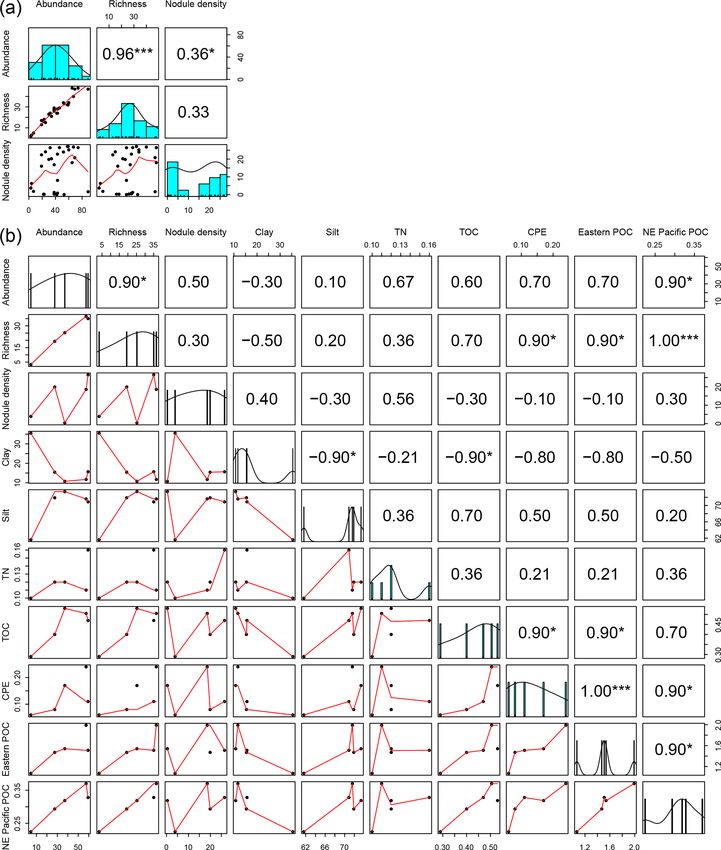
P. Bonifácio et al.: Alpha and beta diversity patterns of polychaete assemblages                                             867

sulted in the designation of nine APEIs (Lodge et al., 2014).     and 5000 m (Fig. 1). The four exploration areas were li-
However, most of the CCFZ had already been preempted by           censed by the ISA to the Federal Institute for Geosciences
current exploration contracts and areas reserved for future       and Natural Resources of Germany (BGR); the InterOcean-
exploration. Consequently, the APEIs were located at the pe-      Metal Joint Organization (IOM); the G-TEC Sea Mineral Re-
riphery of the CCFZ, thus deviating from an optimal design.       sources NV (GSR); and the Institut Français de Recherche
   The European project Managing Impacts of Deep-seA re-          pour l’Exploitation de la Mer (Ifremer). Furthermore, the
Source exploitation (MIDAS) and the Joint Programming             ISA administrates APEI no. 3 as part of the regional envi-
Initiative Healthy and Productive Seas and Oceans (JPI            ronmental plan for the CCFZ. The distances separating the
Oceans) pilot action “Ecological aspects of deep-sea mining”      areas ranged from 243 km (BGR to IOM) to 1440 km (BGR
was aimed at improving the scientific basis on which to as-       to Ifremer or APEI no. 3).
sess and manage the potential impacts arising from nodule
mining. In this context, four exploration contract areas and      2.2   Sampling strategy
one APEI (separated by 240 to 1440 km) were sampled along
a sea surface primary productivity gradient from southeast        The sampling strategy resulted from a combination of objec-
to northwest across the eastern portion of the CCFZ nodule        tives that were unique to each area, together with the over-
province (Martínez Arbizu and Haeckel, 2015). The four ex-        arching aim of describing alpha and beta diversity patterns
ploration contract areas were located within the eastern cen-     across a productivity gradient that included both contract ar-
tral subregion defined by Wedding et al. (2013), where an         eas for nodule exploration and an APEI (Martínez Arbizu
APEI did not fit. One of the nearest APEIs was thus sampled       and Haeckel, 2015). In the BGR area, two sub-areas were
instead.                                                          sampled: a Prospective Area (PA) that could be mined in
   The aims of our study were (i) to test the hypotheses that     the future and a Reference Area (RA) that could serve as
support spatial conservation planning in the CCFZ, partic-        a preservation area. In the IOM area, three sub-areas were
ularly the environmental drivers of alpha and beta diver-         sampled: one that had been directly disturbed by a Benthic
sity such as organic carbon fluxes to the seafloor and nod-       Impact Experiment (BIE; Radziejewska, 2002), one that had
ule density; (ii) to assess the representativeness of an APEI     been impacted by the plume and one undisturbed control
(i.e., APEI no. 3); and (iii) to improve the assessment of po-    area. These levels of sampling stratification are, however, out
tential risks of biodiversity loss due to nodule mining. To       of the scope of the present study, which focuses on variations
tackle these issues, we focused on polychaete assemblages.        between contract areas. After checking that there was no sta-
Polychaetes are the dominant and most diverse group of the        tistically significant difference in the abundance and richness
macrofauna; they can be quantitatively sampled and identi-        of polychaetes between sub-areas, all samples within an area
fied down to species level using a combination of morpho-         were deemed representative of that area and considered repli-
logical and molecular methods (Hessler and Jumars, 1974;          cate samples. The level of replication within areas accord-
Janssen et al., 2015; Wilson, 2017). Polychaetes also show a      ingly varied as a function of sampling stratification. The aim
wide range of biological traits, from trophic behaviors to life   was to collect a minimum of five replicate samples per strata,
history strategies, and play a major role in the functioning of   but due to sampling failures and time constraints it could not
benthic communities (Hutchings, 1998; Jumars et al., 2015).       be systematically achieved (Table 1).
                                                                     Within each area, macrofaunal samples were collected us-
                                                                  ing a United States Naval Electronics Laboratory (USNEL)
2     Materials and methods                                       spade box corer of 0.25 m2 (Hessler and Jumars, 1974).
                                                                  A total of 34 box cores were sampled, of which 30 sam-
2.1    Clarion-Clipperton Fracture Zone                           ples were deemed quantitative (Table 1). The overlying wa-
                                                                  ter was siphoned and sieved using a sieve of 300 µm mesh
The CCFZ is located in the equatorial Pacific Ocean be-           size. The box core sample surface was photographed, and all
tween the Clarion Fracture to the north and the Clipperton        nodules were picked up from the sediment surface, washed
Fracture to the south and between Kiribati to the west and        with cold seawater over a 300 µm mesh sieve and individ-
Mexico to the east (Fig. 1). This area covers about 6 mil-        ually weighed. Sessile and crevice-inhabiting polychaetes,
lion km2 and is composed of a high variety of habitats such       if present, remained with the nodules and were not consid-
as abyssal hills or seamounts, as well as polymetallic nodule     ered in this study. According to Thiel et al. (1993), who
fields (Glover et al., 2016). As part of the JPI Oceans project   washed and broke 26 nodules, the fraction of crevice inhab-
“Ecological aspects of deep-sea mining”, the EcoResponse          itant polychaetes has low significance and representativity
cruise SO239 took place from 11 March to 30 April 2015            (i.e., only 29 specimens belonging to six species) when com-
aboard the RV Sonne (Martínez Arbizu and Haeckel, 2015).          pared with those living in sediments surrounding the nod-
Sampling during the cruise focused on four exploration con-       ules (i.e., 864 polychaetes). The upper 10 cm of each core
tract areas in addition to APEI number 3 (APEI no. 3;             was sliced into three layers (0–3, 3–5 and 5–10 cm) to facili-
Fig. 1). All five study areas had water depths between 4000       tate sieving and sorting; each layer was transferred into cold

www.biogeosciences.net/17/865/2020/                                                        Biogeosciences, 17, 865–886, 2020
Alpha and beta diversity patterns of polychaete assemblages across the nodule province of the eastern Clarion-Clipperton Fracture Zone equatorial ...
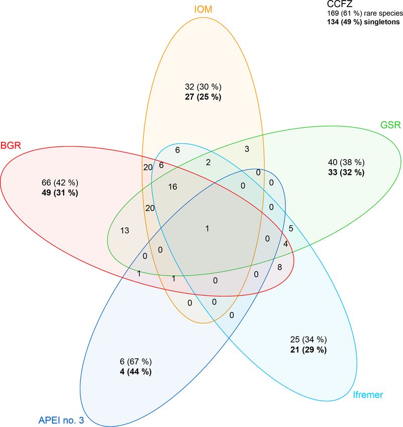
868                                           P. Bonifácio et al.: Alpha and beta diversity patterns of polychaete assemblages

Figure 1. (a) Map of the nodule exploration contracts, reserved areas and Areas of Particular Environmental Interest (APEIs) in the Clarion-
Clipperton Fracture Zone (CCFZ), showing the sampling areas from this study (in color) and previous macrobenthic surveys. The background
map shows the average particulate organic carbon (POC) flux at the seafloor during the 2002–2018 period. The areas sampled during the
SO239 cruises are enlarged in the following panels: BGR (b, c), IOM (d), GSR (e), Ifremer (f) and APEI no. 3 (g). Each has a detailed local
hydroacoustic map based on the multibeam system EM122 (Martínez Arbizu and Haeckel, 2015; Greinert, 2016) in background.

Biogeosciences, 17, 865–886, 2020                                                               www.biogeosciences.net/17/865/2020/
Alpha and beta diversity patterns of polychaete assemblages across the nodule province of the eastern Clarion-Clipperton Fracture Zone equatorial ...
P. Bonifácio et al.: Alpha and beta diversity patterns of polychaete assemblages                                                                869

Table 1. Details of sampling, nodule density, total number of polychaete specimens (ind., individuals by box core) and number of polychaete
species of all 34 box corer deployments across the CCFZ during the SO239 cruise. ∗ indicates box cores considered nonquantitative and thus
not included in the analyses.

 Area         Locality      Station           Date   Depth      Latitude         Longitude   Nodule density   Total abundance    Number of species
                                      (dd/mm/yyyy)     (m)                                       (kg m−2 )    (ind. 0.25 m−2 )     (taxa 0.25 m−2 )
 BGR          BGR-PA            12        20/03/15   4118    11.8471667     −117.05933               26.40                 32                   24
 BGR          BGR-PA            15        21/03/15   4133    11.8443333     −117.05217               26.80                 67                   40
 BGR          BGR-PA            16        21/03/15   4122    11.8573333       −117.052               24.00                 52                   34
 BGR          BGR-PA            21        22/03/15   4120        11.8535     −117.0595               22.80                 43                   28
 BGR          BGR-PA            23        22/03/15   4122          11.85    −117.05267               20.80                 69                   47
 BGR          BGR-RA           51∗        27/03/15   4348    11.8236667     −117.52367                0.00                 22                   12
 BGR          BGR-RA            57        28/03/15   4370        11.8075    −117.52433                8.00                 43                   24
 BGR          BGR-RA            58        28/03/15   4350        11.8205    −117.54167                1.60                 89                   47
 BGR          BGR-RA            60        29/03/15   4325    11.8076667     −117.55033               18.00                 65                   48
 IOM          IOM-control       88        02/04/15   4433         11.079    −119.65883                0.00                 53                   33
 IOM          IOM-control       89        02/04/15   4437    11.0758333     −119.66083                1.20                 38                   29
 IOM          IOM-control       90        03/04/15   4434         11.074    −119.66417                0.00                 42                   24
 IOM          IOM-disturb       94        03/04/15   4414    11.0736667      −119.6555                0.40                 38                   28
 IOM          IOM-disturb       95        03/04/15   4418        11.0735    −119.65583                0.80                 43                   28
 IOM          IOM-disturb       97        04/04/15   4421    11.0728333     −119.65617                0.20                 22                   16
 IOM          IOM-plume       105∗        05/04/15   4423    11.0711667     −119.65533                0.00                 13                    9
 IOM          IOM-plume        106        05/04/15   4425    11.0716667     −119.65483                0.20                 23                   18
 IOM          IOM-plume        107        05/04/15   4425    11.0721667      −119.6545                0.30                 38                   26
 GSR          GSR              119        08/04/15   4516    13.8591667     −123.25267               26.47                 46                   29
 GSR          GSR              127        09/04/15   4514    13.8443333       −123.246               27.10                 59                   32
 GSR          GSR              128        09/04/15   4511    13.8516667       −123.252               27.10                 58                   32
 GSR          GSR              137        11/04/15   4510         13.856      −123.238               25.20                 60                   34
 GSR          GSR              138        11/04/15   4503    13.8481667     −123.23467               26.47                 74                   48
 Ifremer      Ifremer          159        15/04/15   4921         14.049    −130.13433               19.80                 30                   23
 Ifremer      Ifremer          162        16/04/15   4951         14.049      −130.126               20.20                 34                   21
 Ifremer      Ifremer          169        17/04/15   4964    14.0421667     −130.12733               24.10                 25                   15
 Ifremer      Ifremer          180        18/04/15   4936    14.0416667     −130.13633               16.00                 19                   17
 Ifremer      Ifremer          181        18/04/15   4896        14.0465     −130.1415               16.80                 38                   27
 Ifremer      Ifremer          182        18/04/15   4957    14.0423333      −130.1275               22.40                 19                   13
 APEI no. 3   APEI no. 3       195        21/04/15   4833    18.7958333     −128.36217                6.28                  4                    3
 APEI no. 3   APEI no. 3       196        21/04/15   4847    18.7971667     −128.34617                1.80                  7                    5
 APEI no. 3   APEI no. 3      203*        23/04/15   4843         18.774    −128.35317                2.88                  3                    2
 APEI no. 3   APEI no. 3       204        23/04/15   4816    18.7733333     −128.33617                3.65                  3                    2
 APEI no. 3   APEI no. 3      209*        24/04/15   4819        18.7845     −128.3725                3.65                  3                    3

seawater (4 ◦ C) and sieved using the same mesh size. The 0–               2.3     DNA extraction, amplification, sequencing and
3 cm layer was immediately sieved in the cold room with cold                       alignment
seawater (4 ◦ C). The sieve residues from the overlying water
and nodule washing were added to the 0–3 cm layer and live
sorted. All polychaete specimens were photographed, indi-                  The DNA of the subsampled tissues was extracted using
vidualized and preserved in cold (−20 ◦ C) 80 % ethanol and                a NucleoSpin Tissue kit (Macherey-Nagel), following the
then kept at −20 ◦ C (DNA-friendly). The 0–3 cm residue and                manufacturer’s protocol. Approximately 450 base pairs (bp)
3–5 and 5–10 cm layers were fixed in formalin for 48 to 96 h,              of 16S, 700 bp of COI (cytochrome c oxidase subunit I)
preserved in 96 % ethanol, and later sorted in the laboratory              and 1600 bp of 18S genes were amplified using the follow-
(not DNA-friendly). All layers were combined for the com-                  ing primers: Ann16SF and 16SbrH for 16S (Palumbi, 1996;
munity analysis. In the laboratory, from each DNA-friendly                 Sjölin et al., 2005); polyLCO, polyHCO, LCO1490, and
polychaete specimen and from very few fragments, a small                   HCO2198 for COI (Folmer et al., 1994; Carr et al., 2011);
piece of tissue was dissected, fixed in cold 96 % ethanol and              and 18SA, 18SB, 620F, and 1324R for 18S (Medlin et al.,
frozen at −20 ◦ C for molecular studies. DNA sequences from                1988; Cohen et al., 1998; Nygren and Sundberg, 2003) for
fragments without a head were archived in BOLD and Gen-                    18S. The polymerase chain reaction (PCR) mixtures of 25 µL
Bank (Bonifácio et al., 2019) but were not further used for                contained 5 µL of Green GoTaq® Flexi Buffer (final concen-
the purpose of this paper.                                                 tration of 1x), 2.5 µL of MgCl2 solution (final concentration
                                                                           of 2.5 mM), 0.5 µL of PCR nucleotide mix (final concentra-
                                                                           tion of 0.2 mM of each dNTP), 9.875 µL of nuclease-free wa-
                                                                           ter, 2.5 µL of each primer (final concentration of 1 µM), 2 µL

www.biogeosciences.net/17/865/2020/                                                                      Biogeosciences, 17, 865–886, 2020
Alpha and beta diversity patterns of polychaete assemblages across the nodule province of the eastern Clarion-Clipperton Fracture Zone equatorial ...
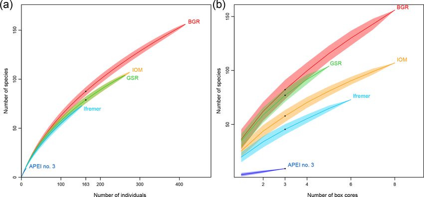
870                                         P. Bonifácio et al.: Alpha and beta diversity patterns of polychaete assemblages

template DNA and 0.125 U of GoTaq® G2 Flexi DNA Poly-              2.5     Environmental data
merase (Promega). The temperature profile for PCR amplifi-
cation consisted of the following steps: initial denaturation at   Environmental data were compiled from Hauquier et
95 ◦ C for 240 s, 35 cycles of denaturation at 94 ◦ C for 30 s,    al. (2019) and Volz et al. (2018). Sediment samples were
annealing at 52 ◦ C for 60 s, extension at 72 ◦ C for 75 s, and    collected with a multi-corer or a gravity corer during the
a final extension at 72 ◦ C for 480 s. Particularly for COI, 40    same cruise and in the same areas (see Martínez Arbizu
cycles were run, and for 18S extension during cycles lasted        and Haeckel, 2015 for details). The sediment characteris-
180 s. PCR products, visualized after electrophoresis on 1 %       tics studied by Hauquier et al. (2019) included a clay frac-
agarose gel, were sent to the MacroGen Europe Laboratory           tion (< 4 µm), a silt fraction (4–63 µm), total nitrogen (TN
in Amsterdam (the Netherlands) to obtain sequences, using          in weight %), total organic carbon (TOC in weight %) and
the same set of primers as used for the PCR.                       chloroplastic pigment equivalents (CPEs in µg mL−1 ). Nod-
   Overlapping sequence (forward and reverse) fragments            ules were weighed onboard for each box-core sample to
were aligned into consensus sequences using Geneious               calculate nodule density (kg m−2 ; Table 1). Particulate or-
Pro 8.1.7 (2005–2015; Biomatters Ltd). For COI, the se-            ganic carbon flux (POC, mg C m−2 d−1 ) at the seafloor for
quences were translated into amino-acid alignments and             our studied areas (eastern CCFZ) were provided by Volz
checked for stop codons to avoid pseudogenes. The mini-            et al. (2018). At the northeastern (NE)-Pacific-Basin scale,
mum length coverage was 207 bp for 16S, 327 bp for COI             POC flux (mg C m−2 d−1 ) at the seafloor was approximated
and 1615 bp for 18S.                                               using net surface primary production provided by the ocean
   The sequences were blasted in GenBank to check for the          productivity site (Westberry et al., 2008) averaged over the
presence of contamination. Each set of genes was aligned           years 2002 to 2018 and applying the Suess algorithm (POC
separately using the following plugins: MAAFT (Katoh et            at the seafloor as a function of the net primary production
al., 2002) for 16S and 18S and MUSCLE (Edgar, 2004)                scaled by depth; Suess, 1980; Table 2). POC flux at seafloor
for COI. All sequences obtained in this study have been            was considered a proxy for food supply to benthic communi-
deposited in BOLD (http://www.boldsystems.org, last ac-            ties.
cess: 12 February 2020; Ratnasingham and Hebert, 2007)
or GenBank (http://www.ncbi.nlm.nih.gov/genbank/, last ac-         2.6     NE-Pacific-scale polychaete community data
cess: 12 February 2020).
                                                                   To put the results of our study in the larger context of the
2.4   Taxonomic identification and feeding guilds                  NE Pacific Basin, we compiled data from previous surveys
      classification                                               of polychaete assemblages in the NE Pacific, including CLI-
                                                                   MAX II sampled in 1969, DOMES A, B and C in 1977 and
Preserved specimens were examined under a Leica M125               1978, ECHO I in 1983, PRA in 1989, EqPac in 1992, Ka-
stereomicroscope and a Nikon Eclipse E400 microscope,              plan East in 2003, Kaplan West and Central in 2004, KR5 in
counted (anterior ends only) and morphologically identified        2012, 2013 and 2014 and GSRNOD15A (B4N01, B4S03 and
using the deep-sea polychaete fauna bibliography (Fauchald,        B6S02) in 2015 (Paterson et al., 1998; Glover et al., 2002;
1972, 1977; Böggemann, 2009) at the lowest taxonomic               Wilson, 2017; Smith et al., 2008b; De Smet et al., 2017).
level possible (morphospecies). We separated closely related       From these studies, we compiled (when available) the mean
species (specimens that could not be discriminated mor-            abundance (ind. 0.25 m−2 ), total number of species, ES163
phologically) using the principle of phylogenetic species,         and bootstrap (Table 2).
whereby the genetic divergence among specimens belong-
ing to the same species (intraspecific) is smaller than the        2.7     Data analysis
divergence among specimens from different species (inter-
                                                                   2.7.1    Univariate analyses
specific) (Hebert et al., 2003a). In the distribution of pair-
wise divergences among all sequences of a typical bar code         Abundance and number of species per box core (Table 1)
dataset, a gap can be observed between intraspecific and in-       and averaged by area (Table 2) were used as descriptors of
terspecific variations. Molecular operational taxonomic units      alpha diversity. A few cryptic or damaged specimens that
(MOTUs) were generally recognized using a threshold of             could not be classified to a lower taxonomical level were
97 % or 99 % similarity between COI and 16S sequences, re-         included in total abundance calculations but excluded from
spectively (Hebert et al., 2003a, b; Brasier et al., 2016). The    subsequent diversity analyses. To compare diversity among
similarity of sequences within species was considered when         the studied areas and for all samples (eastern CCFZ), rar-
identifying morphologically similar species. As genetic data       efaction curves were computed based on the total num-
were only used to separate closely related species, the delim-     ber of individuals and the total number of box core sam-
ited taxa entities in the present study are referenced as mor-     ples (Hurlbert, 1971; Gotelli and Colwell, 2001). Based on
phospecies. Trophic guilds were determined at family level         these data the expected number of species was calculated
following Jumars et al. (2015).                                    for 12 individuals (ES12) and 163 individuals (ES163), as

Biogeosciences, 17, 865–886, 2020                                                          www.biogeosciences.net/17/865/2020/
Alpha and beta diversity patterns of polychaete assemblages across the nodule province of the eastern Clarion-Clipperton Fracture Zone equatorial ...
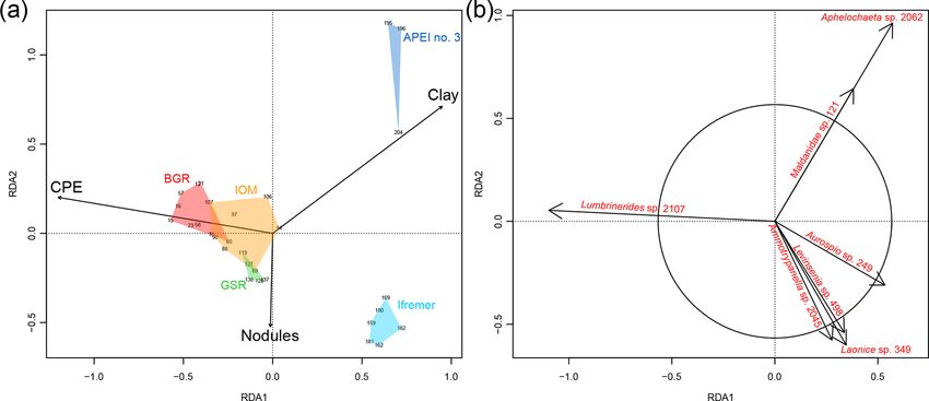
P. Bonifácio et al.: Alpha and beta diversity patterns of polychaete assemblages                                                                                             871

                                                                                                                                                                                                                                     well as for three samples (S3). Nonparametric estimators of
                                                                                                                    2002–2018 average POC at the
                                                                                                                          seafloor (g C m−2 yr−1 )
                                                                                                                                                     1.46

                                                                                                                                                                        1.50
                                                                                                                                                                        1.88
                                                                                                                                                                        1.90
                                                                                                                                                                        2.04

                                                                                                                                                                                               2.05

                                                                                                                                                                                                                  2.11
                                                                                                                                                                                                                  2.04
                                                                                                                                                                                                                  2.11
                                                                                                                                                                                                                  2.11
                                                                                                                                                                                                                  2.07
                                                                                                                                                                                                                  2.27
                                                                                                                                                                                                                  2.23
                                                                                                                                                                                                                  1.66
                                                                                                                                                                                                                  1.91
                                                                                                                                                                                                                  3.55
                                                                                                                                                                                                                  2.68
                                                                                                                                                                                                                  2.33
                                                                                                                                                                                                                  1.78
                                                                                                                                                                                                                                     species richness were used to estimate the total number of
                                                                                                                                                                                                                                     species at local and regional scales. Abundance-based esti-
                                                                                                                                                                                                                                     mators included Chao1 and abundance-based coverage esti-
                                                                                                                                                                                                                                     mator (ACE; O’Hara, 2005; Chiu et al., 2014). Incidence-
                                                                                                                                                                                                                                     based estimators included Chao2 (Chao, 1984), first- and
                                                                                                                                                                                                                                     second-order Jackknife (Burnham and Overton, 1979), and
                                                                                                                                                                                                                                     bootstrap (Smith and van Belle, 1984). A Venn diagram was
                                                                                                                                                                                                                                     used to show the distribution of rare, wide and common
                                                                                                                                                                                                                                     species across the CCFZ.
                                                                                                                                                                                                                                        Univariate analyses relied on nonparametric tests. The
                                                                                                                    Bootstrap

                                                                                                                                                                  203

                                                                                                                                                                               91

                                                                                                                                                                                         310

                                                                                                                                                                                                            274

                                                                                                                                                                                                                    126
                                                                                                                                                                                                                    131

                                                                                                                                                                                                                          192
                                                                                                                                                                                                                           11
                                                                                                                                                                                                                                     Kruskal–Wallis rank sum test was used to test differences
                                                                                                                                                                                                                                     among areas (Hollander and Wolfe, 1973); and the Conover
                                                                                                                                                                                                                                     multiple pairs rank comparisons (adjusted p value by Holm)
                                                                                                                    ES163

                                                                                                                                                     56

                                                                                                                                                                                    47

                                                                                                                                                                                               60

                                                                                                                                                                                                                    79
                                                                                                                                                                                                                    79

                                                                                                                                                                                                                          88

                                                                                                                                                                                                                                71
                                                                                                                                                                                                                                82
                                                                                                                                                                                                                                75
                                                                                                                                                                                                                                     was used to identify the pairs showing differences (Conover
                                                                                                                                                                                                                                     and Iman, 1979; Holm, 1979). Spearman correlations were
                                                                                                                                                                                                                                     sought between biotic and abiotic variables, using data from
                                                                                                                    Total number
                                                                                                                       of species
                                                                                                                                                     104

                                                                                                                                                                                73
                                                                                                                                                                               100

                                                                                                                                                                                               113

                                                                                                                                                                                                                   12
                                                                                                                                                                                                                   10
                                                                                                                                                                                                                   14
                                                                                                                                                                                                                  104
                                                                                                                                                                                                                  107

                                                                                                                                                                                                                          156
                                                                                                                                                                                                                            9
                                                                                                                                                                                                                           46
                                                                                                                                                                                                                           73
                                                                                                                                                                                                                           82
                                                                                                                                                                                                                           76
                                                                                                                                                                                                                           23
                                                                                                                                                                                                                                     the SO239 cruise in the CCFZ and data compiled from the
                                                                                                                                                                                                                                     literature. The latter analysis aimed to test correlations be-
                                                                                                                                                                                                                                     tween biotic variables and POC fluxes at the regional scale.
                                                                                                                    Mean abundance
                                                                                                                     (ind. 0.25 m−2 )
                                                                                                                                                     16

                                                                                                                                                                         5
                                                                                                                                                                        21
                                                                                                                                                                        28
                                                                                                                                                                        65

                                                                                                                                                                                               42

                                                                                                                                                                                                                  20
                                                                                                                                                                                                                  14
                                                                                                                                                                                                                  21
                                                                                                                                                                                                                  59
                                                                                                                                                                                                                  37
                                                                                                                                                                                                                  21
                                                                                                                                                                                                                  58
                                                                                                                                                                                                                   5
                                                                                                                                                                                                                  16
                                                                                                                                                                                                                  84
                                                                                                                                                                                                                  60
                                                                                                                                                                                                                  80
                                                                                                                                                                                                                  13

                                                                                                                                                                                                                                     2.7.2   Multivariate analyses
Table 2. Data available from previous studies and from the present study included in NE-Pacific-scale analyses.

                                                                                                                                                                                                                                     Three indices of faunal similarity were used in multivariate
                                                                                                                                                                                                                                     analyses, the Chord-Normalized Expected Species Shared
                                                                                                                                                                                                                                     (CNESS), the New Normalized Expected Species Shared
                                                                                                                                                                                                                                     (NNESS; Trueblood et al., 1994; Gallagher, 1996) and the
                                                                                                                    Number of
                                                                                                                     box cores
                                                                                                                                                     47
                                                                                                                                                     41

                                                                                                                                                                                6
                                                                                                                                                                               16

                                                                                                                                                                                               15
                                                                                                                                                                                               14
                                                                                                                                                                                                4
                                                                                                                                                                                                5
                                                                                                                                                                                                3
                                                                                                                                                                                                5
                                                                                                                                                                                                8

                                                                                                                                                                                                                           8
                                                                                                                                                                                                                           3
                                                                                                                                                                                                                          10
                                                                                                                                                                                                                           3
                                                                                                                                                                                                                           4
                                                                                                                                                                                                                           3
                                                                                                                                                                                                                           3

                                                                                                                                                                                                                                     Jaccard family indices (Baselga, 2010; Legendre, 2014). The
                                                                                                                                                                                                                                     CNESS and NNESS were computed from probabilities of
                                                                                                                                                                                                                                     species occurrence in random draws of m individuals, with
                                                                                                                    Longitude

                                                                                                                                                     −150.78333

                                                                                                                                                                        −150.00845
                                                                                                                                                                         −130.109
                                                                                                                                                                        −130.13433
                                                                                                                                                                        −128.31667

                                                                                                                                                                                               −126.41667

                                                                                                                                                                                                                  −125.87147
                                                                                                                                                                                                                  −125.46118
                                                                                                                                                                                                                  −123.29704
                                                                                                                                                                                                                    −123.246
                                                                                                                                                                                                                  −119.66083
                                                                                                                                                                                                                   −119.0495
                                                                                                                                                                                                                  −117.54167
                                                                                                                                                                                                                   −128.3725
                                                                                                                                                                                                                       −155
                                                                                                                                                                                                                       −140
                                                                                                                                                                                                                       −140
                                                                                                                                                                                                                       −140
                                                                                                                                                                                                                       −140

                                                                                                                                                                                                                                     low values of m giving a high weight to dominant species
                                                                                                                                                                                                                                     and high values of m giving a high weight to rare species.
                                                                                                                                                                                                                                     The best trade-off value of m is the one providing the highest
                                                                                                                                                                                                                                     Kendall correlation between the similarity matrix for m = 1
                                                                                                                                                                                                                                     and the similarity matrix for m = m max. The value of m
                                                                                                                    Latitude

                                                                                                                                                     8.45

                                                                                                                                                                           9.55195
                                                                                                                                                                        14.0710333
                                                                                                                                                                            14.049
                                                                                                                                                                             12.95

                                                                                                                                                                                               14.6666667

                                                                                                                                                                                                                  14.1124806
                                                                                                                                                                                                                  14.7064111
                                                                                                                                                                                                                  13.8940389
                                                                                                                                                                                                                  13.8443333
                                                                                                                                                                                                                  11.0758333
                                                                                                                                                                                                                  14.9308333
                                                                                                                                                                                                                     11.8205
                                                                                                                                                                                                                     18.7845
                                                                                                                                                                                                                          28
                                                                                                                                                                                                                           0
                                                                                                                                                                                                                           2
                                                                                                                                                                                                                           5
                                                                                                                                                                                                                           9

                                                                                                                                                                                                                                     max was given by the total abundance of the least abundant
                                                                                                                                                                                                                                     sample considered. CNESS was the distance metric used to
                                                                                                                                                                                                                                     perform a redundancy analysis (RDA; Legendre and Legen-
                                                                                                                                                                                                                                     dre, 2012). The RDA is a constrained multivariate analysis
                                                                                                                    Depth
                                                                                                                      (m)
                                                                                                                                                     5100

                                                                                                                                                                        5000
                                                                                                                                                                        5000
                                                                                                                                                                        4937
                                                                                                                                                                        4800

                                                                                                                                                                                               4500

                                                                                                                                                                                                                  4500
                                                                                                                                                                                                                  4500
                                                                                                                                                                                                                  4500
                                                                                                                                                                                                                  4510
                                                                                                                                                                                                                  4425
                                                                                                                                                                                                                  4000
                                                                                                                                                                                                                  4206
                                                                                                                                                                                                                  4832
                                                                                                                                                                                                                  5010
                                                                                                                                                                                                                  4300
                                                                                                                                                                                                                  4400
                                                                                                                                                                                                                  4400
                                                                                                                                                                                                                  4900

                                                                                                                                                                                                                                     that tested the influence of multiple environmental covari-
                                                                                                                                                                                                                                     ates on multi-specific assemblages. Species contributing sig-
                                                                                                                                                     De Smet et al. (2017)
                                                                                                                                                     De Smet et al. (2017)
                                                                                                                                                     De Smet et al. (2017)

                                                                                                                                                     Paterson et al. (1998)

                                                                                                                                                                                                                                     nificantly to the ordination were plotted out of the equilib-
                                                                                                                                                     Smith et al. (2008b)
                                                                                                                                                     Smith et al. (2008b)

                                                                                                                                                     Smith et al. (2008b)
                                                                                                                                                     Glover et al. (2002)

                                                                                                                                                     Glover et al. (2002)

                                                                                                                                                     Glover et al. (2002)

                                                                                                                                                     Glover et al. (2002)
                                                                                                                                                     Glover et al. (2002)
                                                                                                                                                     Glover et al. (2002)
                                                                                                                                                     Glover et al. (2002)

                                                                                                                                                                                                                                     rium circle in RDA (scaling 1). The best set of environmen-
                                                                                                                                                     Wilson (2017)

                                                                                                                                                     Wilson (2017)

                                                                                                                                                     Wilson (2017)
                                                                                                                                                     Present study

                                                                                                                                                     Present study
                                                                                                                                                     Present study

                                                                                                                                                     Present study
                                                                                                                                                     Present study

                                                                                                                                                                                                                                     tal variables was selected using a forward selection proce-
                                                                                                                    References

                                                                                                                                                                                                                                     dure (Borcard et al., 2011) among the environmental vari-
                                                                                                                                                                                                                                     ables available (see Sect. 2.5): clay fraction, silt fraction,
                                                                                                                                                                                                                                     TN, TOC, CPE, nodule density and POC flux at the seafloor.
                                                                                                                                                                                                                                     Furthermore, when selected variables had more than 80 %
                                                                                                                                                     1977/78

                                                                                                                                                                                                                                     co-correlation, they were excluded, and the selection proce-
                                                                                                                                                                        2004
                                                                                                                                                                        2004
                                                                                                                                                                        2015
                                                                                                                                                                        1989

                                                                                                                                                                                               1982

                                                                                                                                                                                                                  2015
                                                                                                                                                                                                                  2015
                                                                                                                                                                                                                  2015
                                                                                                                                                                                                                  2015
                                                                                                                                                                                                                  2015
                                                                                                                                                                                                                  2003
                                                                                                                                                                                                                  2015
                                                                                                                                                                                                                  2015
                                                                                                                                                                                                                  1969
                                                                                                                                                                                                                  1992
                                                                                                                                                                                                                  1992
                                                                                                                                                                                                                  1992
                                                                                                                                                                                                                  1992
                                                                                                                    Year

                                                                                                                                                                                                                                     dure was started over again. Also, the variance inflation fac-
                                                                                                                                                                                                                                     tor (VIF) was used to verify the possible linear dependency
                                                                                                                                                                        Kaplan Central

                                                                                                                                                                                                                                     among variables in the RDA model.
                                                                                                                                                                        Kaplan West

                                                                                                                                                                                                                  Kaplan East

                                                                                                                                                                                                                  CLIMAX II
                                                                                                                                                     DOMES A

                                                                                                                                                                                                                  APEI no. 3

                                                                                                                                                                                                                                        The NNESS index was used to perform a distance de-
                                                                                                                                                                                               ECHO 1

                                                                                                                                                                                                                  EqPac 0
                                                                                                                                                                                                                  EqPac 2
                                                                                                                                                                                                                  EqPac 5
                                                                                                                                                                                                                  EqPac 9
                                                                                                                                                                        Ifremer

                                                                                                                                                                                                                  B4N01
                                                                                                                                                                                                                  B4S03

                                                                                                                                                                                                                  B6S02

                                                                                                                                                                                                                                     cay analysis in the same way as in Wilson (2017). Dis-
                                                                                                                                                                                                                  BGR
                                                                                                                                                                        PRA

                                                                                                                                                                                                                  GSR
                                                                                                                    Area

                                                                                                                                                                                                                  IOM

                                                                                                                                                                                                                                     tance decay screens for a negative correlation between faunal

                                                                                                                  www.biogeosciences.net/17/865/2020/                                                                                                         Biogeosciences, 17, 865–886, 2020
Alpha and beta diversity patterns of polychaete assemblages across the nodule province of the eastern Clarion-Clipperton Fracture Zone equatorial ...
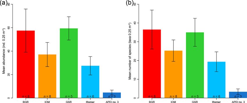
872                                        P. Bonifácio et al.: Alpha and beta diversity patterns of polychaete assemblages

similarities and geographic distances among pairs of areas.       lated with POC flux at the seafloor (rho = 0.75, p < 0.001,
Wilson (2017) used the slope of linear regression between         n = 19; Fig. 4a).
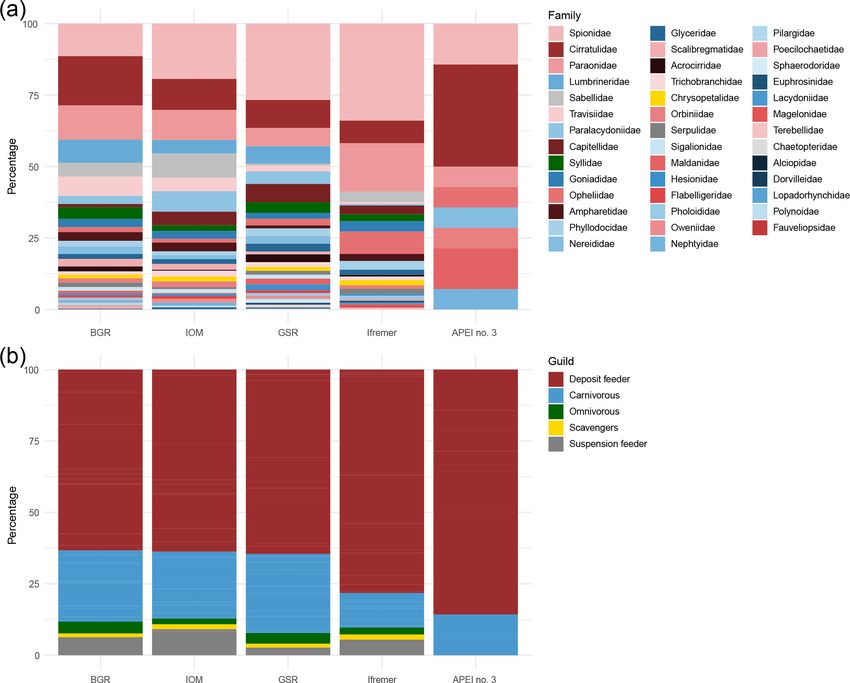
NNESS and distance to compute the rate of change (species            The polychaetes belonged to 41 families (Fig. 5a) with
km−1 ) and the species range (kilometers per species). The        the most abundant being spionids (20 %), cirratulids (13 %),
rate of change is the slope of linear regression between          paraonids (11 %) and lumbrinerids (6 %). Spionids showed
NNESS and distance multiplied by the mean total estimated         the highest relative abundance at the Ifremer (34 %), GSR
species from all areas. The species range is the inverse of the   (27 %) and IOM (19 %) areas, whereas cirratulids were dom-
rate of change.                                                   inant at APEI no. 3 (36 %) and the BGR (17 %) areas. The
   The Jaccard family indices were used to partition beta-        relative contributions of trophic guilds also varied among
diversity into its three components: similarity; turnover,        the areas (Fig. 5b). In particular, carnivores were more com-
which is dissimilarity due to species replacement, and nest-      mon at BGR, IOM and GSR (23 %–28 %) than at Ifremer
edness, which is dissimilarity due to differences in the num-     and APEI no. 3 (12 %–14 %), whereas deposit feeders were
ber of species (Baselga, 2010).                                   overwhelmingly dominant at Ifremer and APEI no. 3 (78 %–
   All analyses were conducted using the R language (R Core       86 %) and less so at BGR, IOM and GSR (63 %–65 %). Sus-
Team, 2018) with RStudio (RStudio Team, 2015) and the fol-        pension feeders, omnivores and scavengers contributed to
lowing specific packages or functions: adespatial (Dray et al.,   less than 13 % of abundance in each area and were not found
2019), BiodiversityR (Kindt and Coe, 2005), fossil (Vavrek,       in APEI no. 3.
2011), vegan (Oksanen et al., 2015), VennDiagram (Chen               Of the 1233 polychaetes, 1118 specimens belonging to 62
and Boutros, 2011), beta.div.comp (Legendre, 2014), ness          genera within 40 families were identified down to morphos-
(Menot, 2019).                                                    pecies. The 115 remaining specimens were too damaged,
                                                                  cryptic or doubtful to be assigned to a morphospecies and
                                                                  were thus not included in diversity and composition analy-
                                                                  ses. The DNA-friendly samples totaled 430 specimens, 265
3     Results                                                     of which were successfully barcoded with either the COI and
                                                                  16S genes (or both). The success rates were 17 % for COI
3.1    Abundance and alpha diversity                              and 60 % for 16S. The COI gene was successfully sequenced
                                                                  for 71 specimens totaling 45 MOTUs; for the 16S gene, 259
During the SO239 cruise, 1233 polychaete specimens were           specimens were successfully sequenced covering 104 MO-
sampled in the five study areas. Interestingly, only a large      TUs; only 65 specimens were successfully sequenced using
specimen identified as Bathyasychis sp. 150 was found             both genes and yielded 40 MOTUs. The 18S gene was se-
deeper than 50 cm (bottom of box core) and thus not included      quenced for phylogenetic purposes on a restricted number of
in the analyses. The dataset has been archived in the infor-      specimens. The 21 sequences of the 18S gene that have been
mation system PANGAEA and is available in open access             obtained are mentioned here because they were archived con-
(Bonifácio et al., 2019).                                         comitantly with COI and 16S sequences in GenBank and
   The mean abundance in each study area tended to de-            BOLD public datasets, but they are not further considered
crease from southeast to northwest, with high variability be-     in this study.
tween neighboring areas (Fig. 2a). Mean densities ranged             Based on both morphological and molecular identifica-
from 58 ± 18 ind. 0.25 m−2 in the BGR area to 5 ± 2 ind.          tion, a total of 275 morphospecies were recognized. The
0.25 m−2 in APEI no. 3. The abundance per box core (Table         mean number of species per area tended to decrease from
1) differed significantly between areas (Kruskal–Wallis test,     southeast to northwest with high variability between neigh-
p < 0.001). The pairwise comparison test (Conover–Holm)           boring areas (Fig. 2b). Mean richness varied from 37 ± 10
showed that (i) APEI no. 3 had significantly lower abundance      taxa 0.25 m−2 in BGR to 3 ± 2 taxa 0.25 m−2 in APEI no. 3.
than the other areas (p ≤ 0.01) except Ifremer, (ii) the Ifre-    The number of species per box core (Table 1) differed sig-
mer exploration area (28 ± 8 ind. 0.25 m−2 ) had significantly    nificantly among areas (Kruskal–Wallis test, p < 0.001). The
lower abundance than the BGR and GSR areas (59 ± 10 ind.          pairwise comparison test (Conover–Holm) showed that the
0.25 m−2 ) (p < 0.001), and (iii) the IOM area (37 ± 10 ind.      number of species per box core was (i) significantly lower
0.25 m−2 ) had significantly lower (p < 0.01) abundance than      at APEI no. 3 than all other areas (p ≤ 0.01) except Ifre-
the BGR and GSR areas. Furthermore, within the eastern            mer, (ii) significantly lower at Ifremer (19±5 taxa 0.25 m−2 )
CCFZ, the abundance per box core was significantly corre-         than at BGR and GSR (35 ± 7 taxa 0.25 m−2 ) (p < 0.001),
lated (Spearman correlations; Fig. 3a) with the number of         and (iii) significantly lower at IOM (25 ± 6 taxa 0.25 m−2 )
species (rho = 0.96, p < 0.001, n = 30) and nodule density        (p < 0.05) than at BGR and GSR. A total of 156 species (ob-
(rho = 0.36, p < 0.05, n = 30); the mean abundance per area       served species richness, Sobs) were sampled at BGR from
was significantly correlated only with POC flux at seafloor       eight box core samples, 107 species at IOM from eight box
(rho = 0.90, p < 0.05, n = 5; Fig. 3b). At the scale of the NE    cores, 104 species at GSR from five box cores, 73 species
Pacific, polychaete abundances were also significantly corre-     at Ifremer from six box cores and 9 species at APEI no. 3

Biogeosciences, 17, 865–886, 2020                                                      www.biogeosciences.net/17/865/2020/
P. Bonifácio et al.: Alpha and beta diversity patterns of polychaete assemblages                                                    873

Figure 2. Bar plots of mean abundance per area (a) and mean species richness per area (b) of polychaete assemblages for each sampled area
within the eastern CCFZ. n indicates the number of box cores samples. Error bars show the standard deviation.

from three box cores (Table 3). Species rarefaction curves,            The first axis of the RDA thus illustrates the influence of
based on individuals or samples, did not reach an asymptote            food inputs on species composition. The clay fraction con-
at the local scale (Fig. 6a, b). Individual-based rarefaction          tributed to the first and the second axis of the RDA. Grain
curves did not show any clear diversity patterns among study           size distribution differentiated APEI no. 3 from all other ar-
areas (Fig. 6a). Sample-based rarefaction curves followed a            eas in the CCFZ (see Hauquier et al., 2019, for details). In
pattern similar to abundance (Fig. 6b). From a random draw             the RDA, the clay fraction accounted for the large dissim-
of three box cores, BGR and GSR, with 82 and 77 species,               ilarity in species composition of the APEI no. 3. Nodule
respectively, had higher expected numbers of species than              density was the main contributor to the second axis of the
IOM and Ifremer did, with 58 and 45 species, respectively.             RDA. Variation in nodule density likely accounted for some
APEI no. 3, with only 9 species, had the lowest expected               of the local variation in species composition. The ordination
number of species (Fig. 6b, Table 3). The nonparametric es-            of species (Fig. 7b) showed that Lumbrinerides sp. 2107 was
timators of local diversity followed the same patterns with            the species most characteristic of the eastern areas; a cirrat-
the highest values for BGR and the lowest for APEI no. 3               ulid (Aphelochaeta sp. 2062) and a maldanid (Maldanidae
(Table 3).                                                             sp. 121) were characteristic of APEI no. 3; and two spionids
   Within the eastern CCFZ, the mean number of species in              (Aurospio sp. 249 and Laonice sp. 349), a paraonid (Levin-
each study area was significantly correlated (Spearman cor-            senia sp. 498), and an opheliid (Ammotrypanella sp. 2045)
relations; Fig. 3b) with POC flux at seafloor (rho = 1.00,             were characteristic of the Ifremer area.
p < 0.001, n = 5) and CPE (rho = 0.90, p < 0.05, n = 5).                  The distance decay of similarity showed two different
At the scale of the NE Pacific, neither ES163 (rho = 0.59,             patterns (Fig. 8a, b). APEI no. 3 had very low values of
p = 0.09, n = 9) nor bootstrap (rho = 0.10, p = 0.8, n = 8)            NNESS compared with all other areas, irrespective of dis-
were correlated with POC flux at the seafloor (Fig. 4b, c).            tance (Fig. 8a). There was no statistically significant cor-
                                                                       relation between NNESS and distance (Radj    2 = 18 %, p =

3.2   Beta and gamma diversity                                         0.12). However, without APEI no. 3, the NNESS values
                                                                       among pairs of exploration contract areas (Fig. 8b) within
In the RDA, the forward selection procedure kept CPE, clay             the CCFZ per se were negatively correlated with distance
                                                                          2 = 0.85, p = 0.006). The slope of the linear regression
                                                                       (Radj
fraction and nodule density as the best explanatory variables.
The model explained 13 % (Radj 2 ) of the total variance in the        (−0.0003) multiplied by the mean of species richness esti-
composition of polychaete assemblages (Fig. 7a). The first             mators for each area (Table 3) provided a rate of species
axis of the RDA discriminated the eastern areas (BGR, IOM              change that ranged from 0.04 species km−1 with the boot-
and GSR) from the western areas (Ifremer and APEI no. 3).              strap estimator (mean species richness of 135 species) to
The second axis of the RDA discriminated Ifremer from                  0.07 species km−1 for the ACE estimator (mean species rich-
APEI no. 3 but also captured local-scale variation because             ness of 234 species). The inverse of these rates of species
replicate samples within areas were distributed along this             change predicted geographic ranges of 14 to 25 km.
second axis. The CPE concentrations mostly explained vari-                Beta diversity was thus high across the CCFZ, particu-
ance along the first axis. CPE was also positively and highly          larly between the exploration contract areas, south of the
correlated with POC flux at seafloor and TOC (Fig. 3b).                Clarion Fracture Zone, and APEI no. 3, north of the Clar-

www.biogeosciences.net/17/865/2020/                                                               Biogeosciences, 17, 865–886, 2020
874                                            P. Bonifácio et al.: Alpha and beta diversity patterns of polychaete assemblages

Figure 3. Correlation matrix between biotic and abiotic variables from sampled areas within the eastern CCFZ. Diagonal plots (a, b) show the
distribution frequency of values for each variable. Panels below the diagonal plots (a, b) show the correlation plot between pairs of variables.
Panels above the diagonal (a, b) plots show the Spearman coefficient correlations between pairs of variables. Abundance, richness and nodule
density per box core are shown in (a) and average biotic and abiotic variables per area are shown in (b). Eastern POC values provided by
Volz et al. (2018); NE Pacific POC values were estimated in the present study. ∗ indicates p < 0.05, ∗∗ ” p < 0.01 and ∗∗∗ p < 0.001.

Table 3. Observed species richness (Sobs) and estimators of species richness for each sampled area and for the eastern CCFZ.

    Area         Sobs               Individual-based                                             Sample-based
                             n     Chao1         ACE      ES12     n      Chao2    Jackknife first   Jackknife second    Bootstrap       S3
                                                                                           order                 order
    BGR           156     415    355 ± 61    334 ± 11   11 ± 1     8   311 ± 46         240 ± 34                  295    192 ± 15     82 ± 9
    IOM           107     274    191 ± 30    225 ± 10   11 ± 1     8   182 ± 26         162 ± 22                  195    131 ± 10     58 ± 6
    GSR           104     263    157 ± 19     196 ± 9   11 ± 1     5   161 ± 20         153 ± 26                  178    126 ± 12     77 ± 6
    Ifremer        73     154    163 ± 38     181 ± 8   11 ± 1     6   160 ± 36         115 ± 19                  142      91 ± 9     45 ± 5
    APEI no. 3      9      12     20 ± 10      27 ± 2    9±0       3    30 ± 27           14 ± 4                   17      11 ± 2      9±0
    CCFZ          275    1118    450 ± 41    484 ± 13   11 ± 1    30   467 ± 44         411 ± 29                  498    334 ± 14    66 ± 13

Biogeosciences, 17, 865–886, 2020                                                                    www.biogeosciences.net/17/865/2020/
P. Bonifácio et al.: Alpha and beta diversity patterns of polychaete assemblages                                                       875

Figure 4. Plot of mean abundance (a) and diversity estimators, ES163 (b) and bootstrap (c), from previous studies and the present study (Ta-
ble 2) in relation to the 2002–2018 average particulate organic carbon (POC) flux at the seafloor along the CCFZ (background). ∗∗∗ indicates
significant (p < 0.001) Spearman correlation.

ion Fracture Zone. In addition, the decomposition of beta di-           4     Discussion
versity showed that dissimilarity was mainly due to species
turnover (91 %) and not nestedness (9 %). However, species              4.1    Major forces driving local- and regional-scale
turnover was driven by singletons. The Venn diagram (Fig. 9)                   patterns in community structure and composition
showed that, in each area, at least 30 % and up to 67 %
of species were unique to one area, so that overall 169                 Food supply, sediment grain size and the density of nodules
out of 275 species were unique to a given area. Of these,               are the three main environmental factors that seem to drive
134 species were singletons (i.e., morphospecies known from             the structure and composition of polychaete assemblages in
a single specimen). Only a single species, Aurospio sp. 249,            the CCFZ.
was sampled in all five areas, 16 species (6 %) were sampled                The abundance of polychaetes per box core was posi-
in four areas, 33 species (12 %) were shared among three ar-            tively correlated with nodule density, which is consistent
eas and 56 species (20 %) were shared between two areas.                with previous studies showing that nodules enhance macro-
   When all individuals and samples were pooled together,               faunal densities and polychaete diversity (De Smet et al.,
rarefaction curves did not level off (Fig. 10a, b) and the num-         2017; Yu et al., 2018). Nodules may have antagonistic in-
ber of singletons steadily increased with increasing sample             fluences on different size groups of benthic communities.
size (Fig. 10b). At this regional scale, nonparametric esti-            Meiofaunal assemblages are less abundant in nodule-rich
mators of species richness ranged from 334 to 498 species               sediments than in nodule-free sediments, which may be due
(Table 3).                                                              to the lower volume of sediment available in nodule areas
                                                                        (Miljutina et al., 2010; Hauquier et al., 2019). In our study,
                                                                        the volume and surface occupied by nodules were not quan-
                                                                        tified but the positive relationship between nodule density
                                                                        and polychaete abundance shows that space is not a limiting

www.biogeosciences.net/17/865/2020/                                                                 Biogeosciences, 17, 865–886, 2020
876                                           P. Bonifácio et al.: Alpha and beta diversity patterns of polychaete assemblages

Figure 5. Bar plots of the relative abundance of families (a) and trophic guilds (b) for each sampled area within the eastern CCFZ. Gradient
color in (a) corresponds to the different guilds in (b).

Figure 6. Rarefaction curves based on individuals (a) and samples (b) for each sampled area within the eastern CCFZ.

factor for polychaetes. Nodules also increase habitat hetero-           ness, thereby increasing friction (Sternberg, 1970; Boudreau
geneity, providing hard substrate for sessile organisms and             and Scott, 1978) and potentially sediment deposition rates.
generally enhancing the standing stocks of both sessile and             The large sessile suspension feeders may similarly enhance
vagile megafauna (Amon et al., 2016; Vanreusel et al., 2016;            biodeposition (Graf and Rosenberg, 1997). Both processes
Simon-Lledó et al., 2019). Nodules increase seafloor rough-             may decelerate water current, stabilizing sediments and thus

Biogeosciences, 17, 865–886, 2020                                                               www.biogeosciences.net/17/865/2020/
P. Bonifácio et al.: Alpha and beta diversity patterns of polychaete assemblages                                            877

Figure 7. Redundancy analysis (RDA) biplot based on the Chord-Normalized Expected Species Shared (CNESS) distance constrained by
the selected variables (a, scaling 2) and showing species significantly contributing to the ordination diagram (b, scaling 1).

Figure 8. Distance decay of New Normalized Expected Species Shared (NNESS) between BGR, IOM, GSR, Ifremer, and APEI no. 3 using
m = 12 (a) and between BGR, IOM, GSR, and Ifremer using m = 50 with regression (y intercept: 0.7642, slope: −0.0002999) (b).

increasing organic carbon supply in the same ways that poly-      in the equatorial northern Pacific (5–15◦ N), with a POC flux
chaete tube lawns do, for example (Friedrichs et al., 2000).      of about 0.5–1.5 g C m−2 yr−1 ; and the oligotrophic abyss
An increase in food supply may explain the higher densities       underlying the North Pacific Subtropical Gyre (15–35◦ N),
of polychaetes in nodule-rich areas.                              with a POC flux lower than 0.5 g C m−2 yr−1 . Our metadata
   At regional to global scales, food input is among the main     analysis confirmed that polychaete abundance was signifi-
forcing factors of the structure and function of the abyssal      cantly and positively correlated with POC flux at seafloor,
ecosystem, which mainly rely upon 0.5 %–2 % of the organic        distinguishing areas in the oligotrophic abyss (APEI no. 3,
carbon derived from sea surface primary production (Rowe et       CLIMAX II, DOMES A, EqPac 9 and Kaplan West) with
al., 1991; Smith et al., 1997; Smith et al., 2008a). Variations   low abundance (4–21 ind. 0.25 m−2 ) from areas in the
in sea surface primary productivity divide the NE Pacific         mesotrophic abyss (Kaplan Central, Ifremer, PRA, ECHO 1,
abyss into three main areas (Sokolova, 1997; Hannides and         GSRNOD15A, GSR, IOM, Kaplan East and BGR) with av-
Smith, 2003; Smith and Demopoulos, 2003): the eutrophic           erage to high abundance (14–85 ind. 0.25 m−2 ) and areas in
abyss in the equatorial upwelling zone (−5◦ S–5◦ N), with         the eutrophic abyss (EqPac 0, 2 and 5) with abundance in the
POC flux of about 1–2 g C m−2 yr−1 ; the mesotrophic abyss        highest range (60–84 ind. 0.25 m−2 ; see Table 2).

www.biogeosciences.net/17/865/2020/                                                        Biogeosciences, 17, 865–886, 2020
878                                           P. Bonifácio et al.: Alpha and beta diversity patterns of polychaete assemblages

                                                                      ture and composition of polychaete assemblages between the
                                                                      APEI no. 3 and the exploration areas echoes that of megafau-
                                                                      nal (Vanreusel et al., 2016), nematode (Hauquier et al., 2019)
                                                                      and tanaid assemblages (Błażewicz et al., 2019). The bio-
                                                                      geochemical settings and the biological patterns of the three
                                                                      size groups of the benthic fauna thus converge to conclude
                                                                      that the structure and functioning of the benthic ecosystem
                                                                      in APEI no. 3 is not representative of any of the four explo-
                                                                      ration contract areas included in this study.
                                                                         Within the mesotrophic zone, the species composition of
                                                                      polychaete assemblages in the Ifremer exploration area dif-
                                                                      fered from the other exploration areas. Differences were
                                                                      driven by species belonging to common deep-sea deposit
                                                                      feeders such as spionids, paraonids and opheliids (Jumars et
                                                                      al., 2015), whereas a lumbrinerid species characterized the
                                                                      eastern exploration areas (BGR, IOM and GSR). Further-
                                                                      more, other carnivorous families were relatively more abun-
                                                                      dant in the eastern areas as well, such as paralacydoniids and
                                                                      sigalionids. These results agree with Smith et al. (2008b)
                                                                      who observed higher abundances of lumbrinerids and am-
                                                                      phinomids, two families of carnivorous polychaetes (Jumars
                                                                      et al., 2015), in the eastern CCFZ (Kaplan East). The up-
Figure 9. Venn diagram with the records of rare (being recorded in    per trophic levels indeed tended to be less represented in the
only one area, with corresponding percentage) and common species      Ifremer and APEI no. 3 areas than in the eastern areas. This
among sampled areas and for the eastern CCFZ. Bold values indi-       pattern matches model predictions that food chain length is
cate the number of species with a single specimen (singletons, with   positively correlated with resource availability in very low
corresponding percentage).                                            productivity systems (< 1–10 g C m−2 yr−1 ; Moore and de
                                                                      Ruiter, 2000; Post, 2002). McClain and Schlacher (2015)
                                                                      formulated this food chain length–productivity relationship
   The exploration areas sampled in our study all lie within          as the “one-more-trophic-level” hypothesis to account for
the mesotrophic zone, but APEI no. 3 lies within the olig-            a positive productivity–diversity relationship. Species rich-
otrophic zone. An analysis of biogeochemical processes con-           ness and productivity were significantly correlated at east-
firmed the very low POC fluxes to the seafloor at APEI no. 3          ern CCFZ scale, but no significant correlation was found be-
(1 mg C m−2 d−1 ) and found respiration rates that were 2-            tween alpha diversity and productivity in the meta-analysis
fold lower than in the exploration areas of the mesotrophic           at the scale of the NE Pacific. The reason diversity and pro-
zone (Volz et al., 2018). APEI no. 3 was also characterized by        ductivity were not correlated in the meta-analysis, which in-
higher clay content, which may be caused by lower sedimen-            cluded data from the literature, could be mainly method-
tation rate and a different sedimentation regime (Hauquier            ological. In particular, the use of integrative taxonomy in
et al., 2019; Volz et al., 2018). Polychaete assemblages in           this study versus morphological taxonomy in previous works
APEI no. 3 consistently showed lower abundance, lower                 might hinder comparisons of diversity metrics.
species richness and lower alpha diversity. Species turnover             To conclude, our study supports the assumptions behind
was also very high, with APEI no. 3 showing the highest               the creation of nine large APEIs, namely that gradients of
rate of species unique to an area and the lowest NNESS                sea surface primary productivity determine large-scale pat-
for all pairs of comparisons. The redundancy analysis also            terns and that nodule densities determine local-scale patterns
suggested that, in addition to food supply, the higher rel-           in community structure, species composition and functioning
ative proportion of clay contributed to variation in species          (Wedding et al., 2013). However, among exploration con-
composition at APEI no. 3. The polychaete assemblage was              tract areas, there is a shift in community composition and
dominated by cirratulids, with one species significantly con-         trophic structure between BGR, IOM, and GSR on the one
tributing to ordination (Aphelochaeta sp. 2062). Some cir-            hand and Ifremer on the other hand, suggesting that these
ratulids are recognized as surface deposit feeders (Jumars            two groups do not belong to the same subregion, as hypoth-
et al., 2015) and may prefer the smaller particles predom-            esized by Wedding et al. (2013). Environmental conditions
inantly present at APEI no. 3 (D4−3 = 15.71 µm). At least             at the APEI no. 3 also seem to be beyond the range of those
two cirratulid species can effectively select particle sizes          found in exploration contract areas, which may explain why
in the clay size range using their tentacles (Magalhães and           the community structure and species composition of benthic
Bailey-Brock, 2017). The strong shift in community struc-             assemblages are so different.

Biogeosciences, 17, 865–886, 2020                                                          www.biogeosciences.net/17/865/2020/
P. Bonifácio et al.: Alpha and beta diversity patterns of polychaete assemblages                                                  879

Figure 10. Rarefaction curves based on individuals (a) and samples (b) within the eastern CCFZ. The dotted curve shows the sample-based
rarefaction curve of singletons.

4.2   Species turnover and geographic ranges                          lantic (Guggolz et al., 2019), or species of Aurospio and Pri-
                                                                      onospio, which could show pan-oceanic distribution (i.e., Pa-
Species turnover was best illustrated by the distance decay           cific and Atlantic oceans; Guggolz et al., 2020). Our obser-
of NNESS similarity, which showed two different patterns.             vations about Aurospio sp. 249, which was the only species
Firstly, APEI no. 3 showed very low similarity with all other         sampled in all five areas, confirm the potential to disperse
areas, irrespective of distance. Secondly, similarity decayed         across large geographic distances of some spionids (Guggolz
linearly with distance among the exploration contract areas           et al., 2020). In the CCFZ, Bonifácio and Menot (2019) de-
located within the CCFZ. Beyond variation in food inputs,             scribed 17 new species of polynoids based on morphology
as discussed above, the large dissimilarity of polychaete as-         and DNA, of which 4 species are shared between APEI no. 3
semblages in APEI no. 3 may suggest a major physiographic             and the exploration areas. In the abyssal Pacific, the CCFZ
barrier between the north and south of the Clarion Fracture.          and the Peru Basin share 9 species of scavenging amphipods,
The Clarion Fracture Zone is a long and narrow submarine              which are highly motile and thus potentially cross the Clip-
mountain range characterized by a peak and trough exceed-             perton and Galapagos fracture zones (Patel et al., 2018).
ing 1800 m difference in elevation (Hall and Gurnis, 2005),           However, species identification was based on morphology
which may be a barrier to dispersal for abyssal fauna. In             only, although cryptic species are common among scaveng-
the Atlantic, the Vema-TRANSIT expedition tested the influ-           ing amphipods, even in abyssal lineages (Brandt et al., 2012;
ence of the Mid-Atlantic Ridge (MAR) and the Vema Frac-               Havermans et al., 2013). The influence of the fracture zones
ture Zone (VFZ) on distribution and connectivity patterns of          on the dispersal of the abyssal fauna remains to be better un-
abyssal fauna with contrasting results (Riehl et al., 2018a).         derstood as the Clarion and Clipperton fractures may act as
The MAR is not a barrier to dispersal for nematode species            a barrier for species with low dispersal abilities, such as in-
of the genus Acantholaimus (Lins et al., 2018), a pattern al-         faunal brooders. If so, the representativeness of seven out of
ready found for 61 copepod species of the genus Mesocle-              the nine APEIs, which lie partly beyond the fractures, may
todes (Menzel et al., 2011). However, the MAR is differ-              be questionable.
ently permeable to dispersal for three families of isopods,              Moreover, the slope of the linear decay of NNESS similar-
depending on their habits and swimming abilities (Bober               ity within the CCFZ suggests an average range of 14 to 25 km
et al., 2018). In particular, connectivity was very low for           per species. This average range masks large variance between
Macrostylidae species, a family of burrowing isopods with             a small pool of widespread species, known from two or more
limited dispersal abilities (Riehl et al., 2018b). The species        areas, and a large pool of rare species, only known from one
composition of the two polychaete families Spionidae and              study area and, in most cases, only known from a single in-
Polynoidae also differed on both sides of the VFZ, which              dividual. This high frequency of singletons may also signifi-
may be due to limited dispersal and different habitat char-           cantly bias the estimation of species ranges (see below for a
acteristics (Guggolz et al., 2018). This was, however, not            discussion on singletons). However, based on the best knowl-
the case for species of Laonice, which tended to show large           edge we have, our study suggests that, on average, the spatial
ranges of up to 4000 km across the eastern and western At-            range of polychaete species in the CCFZ is on the order of

www.biogeosciences.net/17/865/2020/                                                             Biogeosciences, 17, 865–886, 2020
You can also read