POLARIMETRIC GUIDED NONLOCAL MEANS COVARIANCE MATRIX ESTIMATION FOR DEFOLIATION MAPPING
←
→
Page content transcription
If your browser does not render page correctly, please read the page content below
POLARIMETRIC GUIDED NONLOCAL MEANS COVARIANCE MATRIX ESTIMATION
                                                                  FOR DEFOLIATION MAPPING

                                                                 Jørgen A. Agersborg† , Stian Normann Anfinsen† and Jane Uhd Jepsen‡
                                                †
                                                    UiT The Arctic University of Norway, Department of Physics and Technology, Tromsø, Norway
                                                                    ‡
                                                                      Norwegian Institute for Nature Research, Tromsø, Norway
arXiv:2001.08976v2 [eess.IV] 17 Jul 2020

                                                                  1. ABSTRACT                                  work measurements of larvae densities [3]. This follows the
                                                                                                               convention that defoliation studies often are based on NDVI
                                           In this study we investigate the potential for using synthetic      products. A literature review published in 2017 shows that
                                           aperture radar (SAR) data to provide high resolution defolia-       82 % of studies mapping defoliation of broadleaved forest
                                           tion and regrowth mapping of trees in the tundra-forest eco-        caused by insect disturbance used a single spectral index, and
                                           tone. Using aerial photographs, four areas with live forest and     most frequently NDVI [2].
                                           four areas with dead trees were identified. Quad-polarimetric           In this work, we will consider synthetic aperture radar
                                           SAR data from RADARSAT-2 was collected from the same                (SAR) for primarily three reasons. Firstly, polarimetric SAR
                                           area, and the complex multilook polarimetric covariance ma-         data are theoretically able to differentiate between scattering
                                           trix was calculated using a novel extension of guided nonlocal      mechanisms such as surface, volume, and double bounce.
                                           means speckle filtering. The nonlocal approach allows us to         Hence it could be able to accurately separate live tree crowns
                                           preserve the high spatial resolution of single-look complex         (volume scattering) from defoliated trees (double bounce
                                           data, which is essential for accurate mapping of the sparsely       scattering). Secondly, remote sensing products from satellite
                                           scattered trees in the study area. Using a standard random for-     based SAR are near weather-independent. The Norwegian
                                           est classification algorithm, our filtering results in over 99.7%   low arctic tundra has a high average cloud cover percentage,
                                           classification accuracy, higher than traditional speckle filter-    which limits observations by optical satellites. And thirdly,
                                           ing methods, and on par with the classification accuracy based      it would be interesting to evaluate how SAR performs when
                                           on optical data.                                                    it comes to monitor defoliation. While SAR has been used
                                                                                                               to monitor deforestation, none of the studies of broadleaved
                                                               2. INTRODUCTION                                 forest defoliation summarised in [2] used SAR.
                                                                                                                   For remote sensing to contribute to understanding the
                                           The tundra-forest ecotone is the boundary between the low           complicated dynamics of the tundra-forest ecotone, it is im-
                                           arctic tundra and the subarctic forest. A warming climate is        portant that it manages to separate between areas with live
                                           expected to lead to encroachment of woody species into the          and defoliated crown in a setting where trees are sparse and
                                           tundra, however this will be counteracted locally by herbi-         these two classes are interwoven on a fine scale. This leads
                                           vores such as browsing ungulates or defoliating forest pest         to the stringent requirement that we would like to preserve as
                                           insects. Geometrid moth outbreaks cause defoliation and tree        much of the spatial resolution as possible. This again inspired
                                           mortality, and can lead to rapid state transitions of the tundra-   us to extend the guided nonlocal means (GNLM) speckle fil-
                                           forest ecotone. Defoliating species such as geometrids usu-         tering algorithm [4] to estimate complex covariance matrices,
                                           ally do not kill their host tree outright, but inflict damage       preserving the spatial resolution of single-look complex data.
                                           that accumulated over several years, and often in combina-          A random forest classifier was then employed on the filtered
                                           tion with other stressors, leads to an increase in tree mortality   covariance matrices to separate live from defoliated pixels.
                                           [1, 2]. The outbreaks affect large areas, but recovery of the
                                           crown layer of the birch forest is highly dependent on local
                                           factors such as ungulate browsing, soil moisture and quality.          3. DATA COLLECTION AND PREPROCESSING
                                               Remote sensing from satellites provides a valuable con-
                                           tribution by being able to monitor the effects of birch moth        The study area is close to Polmak, Norway and Nuorgam,
                                           outbreaks and the regrowth after for vast areas. The approach       Finland in an area of the subarctic birch forest which stretches
                                           taken in previous work is to detect defoliation based on coarse     across the Norwegian-Finnish border. The effects on the for-
                                           resolution (pixel resolution > 200m) normalised difference          est of a major birch moth outbreak between 2006 and 2008
                                           vegetation index (NDVI) products derived from multispectral         are still clearly visible. By studying high resolution aerial
                                           optical remote sensing images, and correlating this with field      photographs, and comparing images from before (2005) and
NDVI was also calculated, NDVI = (NIR-red)/(NIR+red).
                                                                      Since we are interested in the different scattering phenom-
                                                                   ena, we consider the multilook complex covariance matrix,
                                                                   C. For each pixel, the complex scattering vector is
                                                                                                         T
                                                                                 s = [SHH , SHV , SV V ] ∈ C3×1 ,               (1)
                                                                   where the subscripts indicate the polarisations of the transmit-
                                                                   ted pulse and the received polarisation (horizontal (H) or ver-
                                                                   tical (V)). We have assumed reciprocity, SHV = SV H . Given
                                                                   a set of scattering vectors s, the sample covariance matrix C
                                                                   can be computed as the sample mean, C = hssH i, where the
                                                                   brackets denote averaging and the superscript H the conju-
                                                                   gate transpose operation. In the SNAP software, the speckle
                                                                   filtering step is combined with the estimation of C, where the
                                                                   different speckle filtering algorithms determine how the com-
                                                                   plex scattering vectors used in the average are selected.

                                                                    4. POLARIMETRIC GUIDED NONLOCAL MEANS

                                                                   Nonlocal algorithms are based on splitting the denoising
Fig. 1. Overview of the Polmak study area with reference
                                                                   problem into two steps; 1) Finding good predictors and 2)
areas (rectangles) and transects (red circles).
                                                                   using these predictors in the estimation [5]. While the box-
                                                                   car algorithm makes the implicit assumption that the closest
                                                                   pixels make the best estimators, nonlocal algorithms uses a
after the outbreak (2010), eight reference areas (RAs) were        similarity criterion to find estimators.
identified. All RAs were forested before the outbreak, but              Many different nonlocal algorithms have been used for
four of the eight areas had no live canopy after the outbreak.     speckle filtering, and often the similarity criteria are based on
These were classified as dead and defoliated forest, marked        patch-wise similarity measures for robustness [5]. A further
as blue rectangles in Fig. 1. The remaining four RAs, marked       extension of nonlocal filtering was proposed in [6], where a
in green, represent the live forest class. During fieldwork in     guide image was used to help select similar pixels for aver-
2017, detailed measurements were done for 165 10m × 10m            aging. The guidance image could be the noisy input itself, a
ground plots (red dots in Fig. 1). Six of these are inside three   pre-filtered version of it, or another, coregistered, image [6].
of the RAs. These measurements, while few and not sys-             An example of the former is [7] which used a guided filter-
tematically sampled with respect to the RAs, indicate that the     ing framework to filter the polarimetric covariance matrices,
classes based on the aerial photographs are correctly set.         where the guide used was the noisy SAR image itself.
    Two fine resolution quad-polarisation RADARSAT-2                    The use of a coregistered optical image to guide the SAR
scenes from July 25th and August 1st 2017 were obtained.           despeckling was first proposed in [8]. An important aspect
The nominal scene size is 25km × 25km with a nominal               of the methodology was that the filtered output was the com-
resolution of 5.2m × 7.6m (range × azimuth). Each product          bination of SAR pixels only, to avoid injecting optical image
was radiometrically calibrated and terrain corrected using the     geometry into the SAR scene [8].
European Space Agency (ESA) Sentinel Application Plat-                  Gaetano et al. [9] extended the previous work in [8] to
form (SNAP) software. The terrain corrected output products        use a nonlocal means framework, except for strongly hetero-
had 10.0m × 10.0m spatial resolution.                              geneous areas of the SAR scene. Also [9] improved the earlier
    Next, the data were filtered to suppress the noise-like        results by using patch-based filtering. The need to explicitly
speckle phenomenon inherent to all SAR data. A recent de-          test for heterogeneous areas was replaced by reliability tests
velopment in speckle filtering is the GNLM algorithm, which        which removes unreliable predictors in a further development
uses a co-registered optical image to guide the nonlocal filter-   [4].
ing procedure [4]. For the optical guide image, a Sentinel-2            The previously mentioned work only deals with single-
image from July 26th 2017 covering the study area was ob-          channel intensity SAR images [8, 9, 4], where the filtering
tained from the Copernicus data hub. Atmospheric correction        problem can be formulated as estimating the ”clean” intensity
was applied to retrieve the top of atmosphere reflectance          image X̂ based on the original noisy intensity data X aided by
(TOA). Then all spectral bands with 10.0m spatial resolu-          the coregistered optical guide image O. The filtering is patch-
tion, namely red, green, blue, and near infrared (NIR), were       based, where a patch centred on a pixel with spatial index
extracted. For comparison of classification performance, the       (pixel position) j is defined as x(j) = {X(j + k) , k ∈ P},
where P indicates a set of N spatial offsets with respect to j By modifying Eq. (2), we can then find the polarimetric
[4]. guided nonlocal means (PGNLM) estimate for the covariance
The filtering is then done for each patch x(j) centred on matrix as: X
pixel j in the input SAR image, by summing the weighted C(j) = w(i, j)si sH
i (7)
patches x(i) in a search area Ω(j) around j: i∈Ω(j)
X Where the weight w(i, j) is defined in Eq. (3), dOPT is given
x̂(j) = w(i, j)x(i) (2) in Eq. (4), and dSAR in Eq. (6).
i∈Ω(j)
Note that while each pixel intensity is estimated multiple
where the size of the search area Ω is determined by a pa- times as it is a part of multiple patches in the case of single-
rameter, and the patch size of x̂ and x are equal and given by channel intensity filtering in Eq. (2), the covariance matrix for
P. Since each pixel is part of multiple patches, the filtering pixel position j is only estimated once. The estimate in Eq.
procedure will estimate each pixel multiple times [4]. (7) is based on pixels where the patch P centred on that pixel
Note that the optical data does not enter directly into Eq. is sufficiently similar to the patch centred on the pixel position
(2), which means that only SAR domain pixels are used for to be estimated, and weighted according to the dissimilarities
determining the filtered SAR image [4]. It is only used to help in the SAR and optical domain.
determine the weights w(i, j) in Eq. (2)
The weight determining how much the filtering of a patch 5. RESULTS
centred on pixel j is influenced by patch centred on pixel i
can then be written as: For separating pixels with live crown foliage from those with
defoliated crown, we train a random forest classifier with 200
w(i, j) = Ce−λ[γdSAR (i,j)+(1−γ)dOPT (i,j)] (3) trees on the filtered covariance matrices. For comparison we
obtained the filtered covariance matrices using the boxcar,
where C is a normalising constant, dSAR and dOPT are patch- enhanced Lee, and intensity-driven adaptive-neighbourhood
based dissimilarity measures in the SAR and optical domain (IDAN) filters in SNAP. Both boxcar and enhanced Lee fil-
respectively, λ is an empirical weight parameter, and γ ∈ ters used a 5 × 5 window, while the adaptive-neighbourhood
[0, 1] balances the emphasis on SAR versus optical dissimi- size for IDAN was 50.
larity. The PGNLM parameters were set in a heuristic manner,
For the optical domain, [4] used the normalised sum of following recommendations in [4]. The search area was set to
the squared Euclidean distance 39 × 39 pixels, while the size of the patches to be compared
B were 9 × 9. The balancing factor between SAR and optical
1 XX 2 dissimilarities, γ in Eq. (3) was set to 0.85, while λ was 0.5.
dOPT (i, j) = [ob (i + k) − ob (j + k)] (4)
BN Also the measures to discard unreliable predictors used in [4]
b=1 k∈P
was employed.
where B is the number of bands in the optical guide and N All the polarimetric information is contained in the el-
is the number pixels in each patch determined by the set of ements of C, and we can further simplify the processing
spatial offsets P. by extracting the properties with relevant information: C11 ,
The SAR dissimilarity measure used in [4] was for mul- C22 , C33 , |C13 |, and ∠C13 . Here, C11 , C22 , C33 are the
tiplicative noise in single polarisation intensity data. To ex- intensities in the HH, HV, and VV channels, respectively,
tend GNLM to PolSAR data, we chose to use a dissimilarity and C13 = |C13 |ej∠C13 is the cross-correlation between the
measure that utilised the polarimetric information. Since each complex scattering coefficients in the co-polarised channels
pixel in the input SAR image is a complex scattering vector as HH and VV.
defined in Eq. (1), a dissimilarity measure between two such In addition, we compare with the classification result on
vectors can be defined as the four-band optical Sentinel-2 subset used as the guide in
(sj − si )H (sj − si ) PGNLM, as well as the NDVI. All data were divided into 5
d(si ,sj ) = (5) parts for k-fold cross validation, and the average accuracy is
sHj sj
reported. The result is seen in Figure 2.
If we sum this expression we can get a patch-based dissimilar- We see that PGNLM achieves 100% accuracy for 25
ity between the patches centred on pixel position j and pixel July (red bar), 5.7 percentage points better than second best
position i (IDAN). For the 1 August dataset (blue bar) PGNLM achieves
99.7% accuracy, 6.0 percentage points better than second best
1 X (sj+k − si+k )H (sj+k − si+k ) (IDAN). The optical data (Sentinel-2 25 July), shown in green
dSAR (i, j) = (6)
N
k∈P
sH
j+k sj+k
bars, achieves 99.9% accuracy. As expected, the NDVI result
is significantly lower, as it is based on only two out of four
where N and P are defined as before. bands in the optical image.Fig. 2. Random forest classification accuracy.
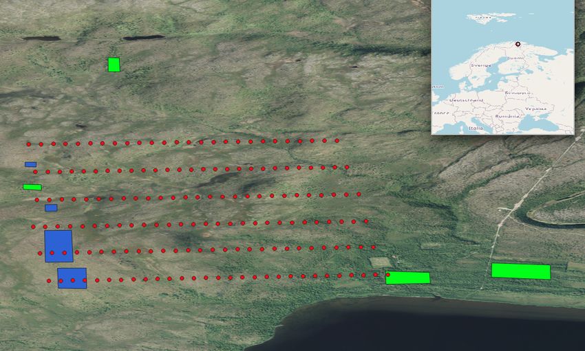
Fig. 3 shows a close-up of an area north of the eastern-
most live RA in Fig. 1. For the SAR data, C11 , C22 , C33 are
normalised and shown in the red, green, and blue channels
respectively. The PGNLM algorithm achieves a significantly
smoother result than the other filtering methods, and without
any obvious filtering artefacts. This is not unexpected as it
averages covariance matrix estimations from a large search
area, while also discarding unreliable predictors.
6. CONCLUSIONS AND FUTURE WORK
PGNLM filtered SAR data achieve the best accuracy results
of the SAR filtering methods, and comparable to optical data. Fig. 3. Optical data (top row) and filtered SAR data.
The PGNLM algorithm contains quite a few parameters,
that in various ways impact each other. Here they were set
[4] S. Vitale, D. Cozzolino, G. Scarpa, L. Verdoliva, and G. Poggi,
in a heuristic manner. For a better understanding, how to set “Guided patchwise nonlocal SAR despeckling,” IEEE Trans.
the parameters for polarimetric guided nonlocal means should Geosci. Remote Sens., vol. 57, no. 9, pp. 6484–6498, 2019.
be explored, as was done for GNLM in [4]. Also, applying
[5] C.-A. Deledalle, L. Denis, G. Poggi, F. Tupin, and L. Verdoliva,
PGNLM to standard datasets can help get a more accurate
“Exploiting patch similarity for SAR image processing: the non-
comparison of its performance relative to other polarimetric local paradigm,” IEEE Signal Process. Mag., vol. 31, no. 4, pp.
speckle filtering methods. 69–78, 2014.
[6] K. He, J. Sun, and X. Tang, “Guided image filtering,” IEEE
7. REFERENCES
Trans. Pattern Anal. Mach. Intell., vol. 35, no. 6, pp. 1397–1409,
[1] J. U. Jepsen, M. Biuw, R. A. Ims, L. Kapari, T. Schott, O. P. L. 2012.
Vindstad, and S. B. Hagen, “Ecosystem impacts of a range ex- [7] X. Ma, P. Wu, and H. Shen, “A nonlinear guided filter for polari-
panding forest defoliator at the forest-tundra ecotone,” Ecosys- metric SAR image despeckling,” IEEE Trans. Geosci. Remote
tems, vol. 16, no. 4, pp. 561–575, 2013. Sens., vol. 57, no. 4, pp. 1918–1927, 2018.
[2] C. Senf, R. Seidl, and P. Hostert, “Remote sensing of forest [8] L. Verdoliva, R. Gaetano, G. Ruello, and G. Poggi, “Optical-
insect disturbances: current state and future directions,” Int. J. driven nonlocal SAR despeckling,” IEEE Geosci. Remote Sens.
Appl. Earth Observ. Geoinf., vol. 60, pp. 49–60, 2017. Lett., vol. 12, no. 2, pp. 314–318, 2014.
[3] J. U. Jepsen, S. B. Hagen, K. A. Høgda, R. A. Ims, S. R. [9] R. Gaetano, D. Cozzolino, L. D’Amiano, L. Verdoliva, and
Karlsen, H. Tømmervik, and N. G. Yoccoz, “Monitoring the G. Poggi, “Fusion of SAR-optical data for land cover monitor-
spatio-temporal dynamics of geometrid moth outbreaks in birch ing,” in Proc. IEEE Int. Geosci. Remote Sens. Symp. (IGARSS).
forest using MODIS-NDVI data,” Remote Sens. Environ., vol. IEEE, 2017, pp. 5470–5473.
113, no. 9, pp. 1939–1947, 2009.You can also read