Predicting the morphology of ice particles in deep convection using the super-droplet method: development and evaluation of SCALE-SDM 0.2.5-2.2.0 ...
←
→
Page content transcription
If your browser does not render page correctly, please read the page content below

Geosci. Model Dev., 13, 4107–4157, 2020
https://doi.org/10.5194/gmd-13-4107-2020
© Author(s) 2020. This work is distributed under
the Creative Commons Attribution 4.0 License.
Predicting the morphology of ice particles in deep convection using
the super-droplet method: development and evaluation of
SCALE-SDM 0.2.5-2.2.0, -2.2.1, and -2.2.2
Shin-ichiro Shima1,2 , Yousuke Sato3,2 , Akihiro Hashimoto4 , and Ryohei Misumi5
1 Graduate School of Simulation Studies, University of Hyogo, Kobe, Japan
2 RIKEN Center for Computational Science, Kobe, Japan
3 Faculty of Science, Hokkaido University, Sapporo, Japan
4 Meteorological Research Institute, Japan Meteorological Agency, Tsukuba, Japan
5 National Research Institute for Earth Science and Disaster Resilience, Tsukuba, Japan
Correspondence: Shin-ichiro Shima (s_shima@sim.u-hyogo.ac.jp)
Received: 16 October 2019 – Discussion started: 11 December 2019
Revised: 13 July 2020 – Accepted: 22 July 2020 – Published: 8 September 2020
Abstract. The super-droplet method (SDM) is a particle- 1 Introduction
based numerical scheme that enables accurate cloud micro-
physics simulation with lower computational demand than Mixed-phase clouds, which are clouds comprising droplets
multi-dimensional bin schemes. Using SDM, a detailed nu- and ice particles, appear under multiple atmospheric condi-
merical model of mixed-phase clouds is developed in which tions, from the tropics to the poles, and throughout the year
ice morphologies are explicitly predicted without assuming (Shupe et al., 2008). Accurately simulating the evolution of
ice categories or mass–dimension relationships. Ice particles droplets and ice particles in mixed-phase clouds is crucial to
are approximated using porous spheroids. The elementary understanding cloud dynamics, precipitation formation, wa-
cloud microphysics processes considered are advection and ter transport, radiative properties, aerosol–cloud interaction,
sedimentation; immersion/condensation and homogeneous cloud electrification, and lightning. These features are all cru-
freezing; melting; condensation and evaporation including cial to many environmental and societal issues, such as cli-
cloud condensation nuclei activation and deactivation; depo- mate change and variability, numerical weather prediction,
sition and sublimation; and coalescence, riming, and aggre- weather modification, and icing on infrastructure (e.g., wind
gation. To evaluate the model’s performance, a 2-D large- turbines and power lines) and aircraft (e.g., Korolev et al.,
eddy simulation of a cumulonimbus was conducted, and 2017).
the life cycle of a cumulonimbus typically observed in na- Through their 70-year history, numerical models of cloud
ture was successfully reproduced. The mass–dimension and microphysics have become increasingly sophisticated (e.g.,
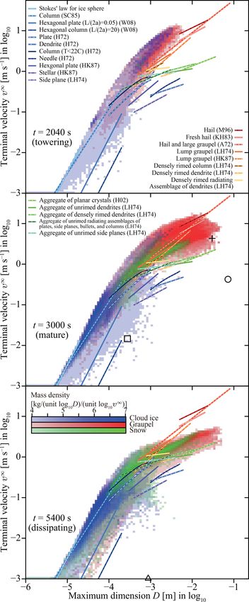
velocity–dimension relationships the model predicted show Khain et al., 2015; Khain and Pinsky, 2018; Grabowski et al.,
a reasonable agreement with existing formulas. Numerical 2019; Morrison et al., 2020). However, recent model inter-
convergence is achieved at a super-particle number concen- comparison studies revealed that the models do not show
tration as low as 128 per cell, which consumes 30 times any sign of converging toward the truth. Even the most so-
more computational time than a two-moment bulk model. phisticated models do not correspond well, and the diver-
Although the model still has room for improvement, these re- gence in model results is as large in sophisticated models
sults strongly support the efficacy of the particle-based mod- as it is in simple models (VanZanten et al., 2011; Xue et al.,
eling methodology to simulate mixed-phase clouds. 2017). Mixed-phase cloud microphysics modeling is partic-
ularly challenging because we still lack a sufficient scientific
understanding of mixed-phase cloud microphysics, and an
algorithm appropriate for mixed-phase cloud microphysics
Published by Copernicus Publications on behalf of the European Geosciences Union.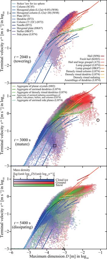
4108                                S. Shima et al.: Predicting morphology of ice particles using the super-droplet method

does not exist. This study aims to address the second prob-        derstanding is not yet sufficient, it is plausible that mixed-
lem.                                                               phase cloud microphysics could be accurately described un-
   Every numerical model is an approximation of a phe-             der a kinetic description framework. Indeed, direct compar-
nomenon’s mathematical model, which is a theoretical de-           ison with laboratory data suggests that a kinetic description
scription that should express the system’s behavior accu-          could express ice particle morphology evolution accurately
rately. We apply a numerical scheme to construct a numerical       (Jensen and Harrington, 2015). This is crucial because ice
model, which we use to produce an approximate solution of          particle morphology significantly influences the fall speed,
the phenomenon’s underlying mathematical model for given           growth by diffusion and collision, and radiative properties of
spatiotemporal boundary conditions. This general philoso-          ice particles. Because of their direct correspondence to ele-
phy of simulation is well documented, e.g., in Stevens and         mentary processes, it should also be easier to refine kinetic
Lenschow (2001).                                                   descriptions using laboratory measurements.
   There are several types of cloud microphysics numerical            Two numerical scheme types exist for kinetic descriptions,
models that are based on different levels of theoretical de-       namely bin schemes and particle-based schemes.
scriptions.                                                           The development of bin schemes started independently of
   The first of these is the bulk model, which is the most         bulk models in the 1950s (e.g., Mason and Ramanadham,
widely used cloud microphysics model type (see, e.g., Khain        1954; Hardy, 1963; Srivastava, 1967). For a review, see, e.g.,
et al., 2015; Morrison and Milbrandt, 2015; Khain and Pin-         Khain et al. (2015), Khain and Pinsky (2018), Grabowski
sky, 2018; Grabowski et al., 2019; Morrison et al., 2020, for      et al. (2019), and Morrison et al. (2020).
a review). Bulk models consider only the particle popula-             Particle-based cloud microphysics modeling is a new ap-
tion’s statistical features and are thus based on macroscopic      proach that has emerged since the mid-2000s (e.g., Paoli
descriptions of cloud microphysics. They solve a mathemati-        et al., 2004; Jensen and Pfister, 2004; Shirgaonkar and Lele,
cal model that is closed in the lower moments of the distribu-     2006; Andrejczuk et al., 2008, 2010; Shima et al., 2009;
tion function of cloud droplets, rain droplets, and ice particle   Sölch and Kärcher, 2010; Riechelmann et al., 2012; Brdar
categories (e.g., mass and number mixing ratios). The basic        and Seifert, 2018; Seifert et al., 2019; Jaruga and Pawlowska,
premise of bulk models is that the distribution function can       2018; Grabowski and Abade, 2017; Abade et al., 2018;
be determined by the lower moments, but such a universal re-       Grabowski et al., 2018; Hoffmann et al., 2019). During
lationship is unknown. In other words, in bulk models, to pre-     particle-based modeling’s early development, calculating the
dict the time evolution of a chosen set of moments, their time     coalescence process was a numerical challenge. Shima et al.
derivatives are approximated by some functions of the mo-          (2009), Andrejczuk et al. (2010), Sölch and Kärcher (2010),
ments being predicted, but this is not generally possible (see,    and Riechelmann et al. (2012) proposed different algorithms,
e.g., Beheng, 2010). It would be also informative to note the      and among those four schemes, the super-droplet method
analogy and difference between the Navier–Stokes equation          (SDM) developed by Shima et al. (2009) provides a com-
and bulk models (Morrison et al., 2020), which highlights          putationally efficient Monte Carlo algorithm (Unterstrasser
the difficulty in deriving bulk models. Therefore, for cloud       et al., 2017; Dziekan and Pawlowska, 2017). Several other
microphysics, a more bottom-up approach to construct more          coalescence algorithms were proposed in different research
accurate and reliable numerical models would be desired.           areas such as the weighted flow algorithm for aerosol dynam-
   Kinetic description provides a more detailed microscopic        ics (DeVille et al., 2011); O’Rourke’s method (1981), and
mathematical model of cloud microphysics, with the evolu-          the no-time counter method (Schmidt and Rutland, 2000) for
tion and motion of individual aerosol, cloud, and precipita-       spray combustion; and Ormel and Spaans’s method (2008)
tion particles being explicitly considered. Assuming that par-     and Johansen et al.’s method (2012) for astrophysics. Li et al.
ticles are locally well mixed, particle collisions are regarded    (2017) confirmed that the performance of SDM is better than
as a stochastic process. Each particle is characterized by its     Johansen et al.’s method (2012), but direct comparison with
position and internal state, the latter of which is specified by   other algorithms remains to be assessed.
variables known as attributes, such as size, mass, ratio of the       The essential difference between bin schemes and particle-
ice crystal’s minor axis to the major axis (hereafter called       based schemes lies in the representation of particles. Bin
“aspect ratio”), velocity, and chemical composition.               schemes adopt an Eulerian approach and the particle dis-
   Mixed-phase cloud microphysics are far more compli-             tribution function is approximated using a finite number of
cated than those of liquid-phase clouds, with various ice          control volumes (histogram). The time evolution is solved
crystal formation mechanisms, diffusional growth by deposi-        using a finite volume method or a finite difference method.
tion/sublimation, diverse ice particle morphologies, ice melt-     In contrast, particle-based schemes rely on a Lagrangian ap-
ing and shedding, riming and wet growth, aggregation, spon-        proach and the population of real particles is approximated
taneous/collisional breakup of ice particles, and rime splin-      by using a population of weighted samples, sometimes re-
tering at play (e.g., Pruppacher and Klett, 1997; Hashino and      ferred to as super-droplets or super-particles. As discussed
Tripoli, 2007, 2008, 2011a, b; Khvorostyanov and Curry,            in Grabowski et al. (2019), bin schemes face problems that
2014; Khain and Pinsky, 2018). Although our scientific un-         are challenging to overcome such as numerical diffusion,

Geosci. Model Dev., 13, 4107–4157, 2020                                            https://doi.org/10.5194/gmd-13-4107-2020

S. Shima et al.: Predicting morphology of ice particles using the super-droplet method                                        4109

computational cost, and the breakdown of the Smoluchowski          SDM. The fluid dynamics of moist air is solved by adopt-
equation (Smoluchowski, 1916; Alfonso and Raga, 2017;              ing a forward temporal integration scheme to both horizontal
Dziekan and Pawlowska, 2017). However, SDM could re-               and vertical directions using a finite volume method with an
solve, or at least mitigate, those problems.                       Arakawa-C staggered grid. To evaluate our model’s perfor-
   Therefore, SDM and similar particle-based schemes               mance, we conduct a two-dimensional (2-D) simulation of
should be more suitable for mixed-phase cloud microphysics         an isolated cumulonimbus, and find that our model well re-
simulations than bin schemes. Mainly because of computa-           produces the life cycle of a cumulonimbus typically observed
tional costs, it is practically impossible to apply bin schemes    in nature. The mass–dimension and velocity–dimension rela-
to the most comprehensive form of kinetic description, which       tionships our model predicts show a reasonable agreement
inevitably involves multiple attributes to express each parti-     with existing formulas based on laboratory measurements
cle’s internal state. Instead, many existing bin models solve      and field observations. We also investigate the simulation’s
a simplified kinetic description that uses particle distribution   numerical convergence and confirm that our model can pro-
functions with a one-dimensional attribute space approxima-        duce an accurate approximate solution with lower computa-
tion. For example, most rely on artificially separated cate-       tional demand than multi-dimensional bin schemes. We then
gories of ice particles, with predefined mass–dimension and        explore the possibility of further refining and sophisticating
area–dimension relationships in each category. Another ap-         the model; however, advancing our understanding of mixed-
proach is adopted in the SHIPS model developed by Hashino          phase cloud microphysics is beyond the scope of this study.
and Tripoli (2007, 2008, 2011a, b), which is a bin model that         Several previous works are closely relevant to this study.
solves sophisticated and comprehensive kinetic descriptions        Chen and Lamb (1994a, b) developed a detailed multi-
and does not use ice categories or mass–dimension relation-        dimensional bin model, which Misumi et al. (2010) ex-
ships. However, to justify using the one-dimensional particle      tended and added ice volume as a new particle attribute.
distribution function, they rely on the “implicit mass sorting     We follow that strategy and approximate ice particles as
assumption”, stating that different solid hydrometeor species      porous spheroids; however, their kinetic description is more
do not belong to the same bin because they are naturally           detailed than ours because they also considered sponta-
sorted by mass. Such simplifications could be a significant        neous/collisional breakup, shedding, rime splintering, and
source of errors. SDM and similar particle-based schemes           surface chemical reactions. They solved the model using a
could directly simulate comprehensive kinetic descriptions         multi-dimensional bin scheme; hence, their numerical model
with lower computational demand.                                   carries a high computational cost. Hashino and Tripoli (2007,
   This study’s primary objective is to assess particle-based      2008, 2011a, b) further extended Chen and Lamb (1994a,
modeling methodology’s capability to simulate mixed-phase          b)’s kinetic description to account for polycrystals that can
clouds. Therefore, we develop and evaluate the performance         form below −20 ◦ C. They solve the mathematical model us-
of a detailed numerical mixed-phase cloud model using              ing a one-dimensional bin scheme; however, careful vali-
SDM, wherein ice particle morphologies are explicitly pre-         dation is needed to justify their implicit mass sorting as-
dicted.                                                            sumption. Paoli et al. (2004), Jensen and Pfister (2004), and
   We first construct a mixed-phase cloud microphysics             Shirgaonkar and Lele (2006) separately developed a particle-
mathematical model, which is based on kinetic description.         based model for ice-phase clouds, but neither the evolution of
The fluid dynamics of moist air is described by the compress-      ice particle morphologies nor the aggregation of ice particles
ible Navier–Stokes equation, and aerosol, cloud, and precip-       were considered in their models. Sölch and Kärcher (2010)
itation particles are represented by point particles. Following    also developed a particle-based model for ice-phase clouds,
Chen and Lamb (1994a, b) and Misumi et al. (2010), ice par-        but that model relies on ice categories and mass–dimension
ticles are approximated using porous spheroids. The elemen-        relationships. Brdar and Seifert (2018) developed McSnow,
tary cloud microphysics processes considered in the model          the first particle-based model for mixed-phase clouds. Mc-
are advection and sedimentation; immersion/condensation            Snow is a multi-dimensional expansion of the P3 bulk model
and homogeneous freezing; melting; condensation and evap-          (Morrison and Milbrandt, 2015; Milbrandt and Morrison,
oration including the cloud condensation nuclei (CCN) acti-        2016) and thus free from ice categories; however, it still re-
vation and deactivation; deposition and sublimation; and co-       lies on mass–dimension relationships. Further, a kinetic ap-
alescence, riming, and aggregation. We base the mathemat-          proach is applied to ice particles but not to droplets or aerosol
ical models used for those elementary processes on revised         particles.
versions of existing formulas. Additionally, our model does           In this study, we demonstrate that a large-eddy simulation
not rely on ice categories or predefined mass–dimension re-        of a cumulonimbus that predicts ice particle morphologies
lationships. For simplicity, and due to the lack of appropri-      without assuming ice categories or mass–dimension relation-
ate algorithms, we do not consider spontaneous/collisional         ships is possible if we use SDM.
breakup or rime splintering. We then develop a numeri-                The organization of the remainder of this paper is as fol-
cal model called SCALE-SDM to solve the mathematical               lows. In Sects. 2–4, our mixed-phase cloud mathematical
model. Mixed-phase cloud microphysics is solved using the          model is described in detail. The cloud microphysics model

https://doi.org/10.5194/gmd-13-4107-2020                                             Geosci. Model Dev., 13, 4107–4157, 2020
4110                                     S. Shima et al.: Predicting morphology of ice particles using the super-droplet method

is based on kinetic description and is coupled with moist                  2.4   Freezing temperature and ice nucleation active
air fluid dynamics. Note that this model is an expansion of                      surface site
Shima et al. (2009)’s warm cloud model. In Sect. 5, we de-
velop a numerical model called SCALE-SDM by applying                       We only consider homogeneous freezing and condensa-
SDM. To evaluate SCALE-SDM’s performance, we conduct                       tion/immersion freezing in this study because these are dom-
a 2-D simulation of an isolated cumulonimbus. Section 6                    inant in mixed-phase clouds (e.g., Cui et al., 2006; De Boer
presents the design of the numerical experiments, and in                   et al., 2011; Murray et al., 2012).
Sect. 7, the overall properties of the simulated cumulonim-                   Based on the “singular hypothesis” (Levine, 1950), we
bus and ice particle morphologies are analyzed. The numeri-                consider that each insoluble particle has its own freezing
cal convergence characteristics of the model are investigated              temperature T fz , and that a supercooled droplet freezes as
in Sect. 8. In Sect. 9, possible improvements of the model are             soon as the ambient temperature T decreases below T fz . The
discussed, and a summary and conclusions are presented in                  freezing process is described in detail in Sect. 4.1.4.
Sect. 10. Lastly, lists of symbols and abbreviations are pro-                 Each particle’s T fz is directly connected to the ice nu-
vided in Appendices A and B, respectively. Note that a com-                cleation active surface site (INAS) density concept (e.g.,
prehensive table of contents is provided as PDF bookmarks.                 Fletcher, 1969; Connolly et al., 2009; Niemand et al., 2012;
                                                                           Hoose and Möhler, 2012).
                                                                              An INAS is a localized structure, such as lattice mis-
2     Attributes of atmospheric particles                                  matches, cracks, and hydrophilic sites, on an insoluble sub-
                                                                           stance’s surface that catalyzes ice formation at temperatures
2.1    Notion of a particle                                                lower than a specific temperature. INAS density nS (T ) gives
                                                                           the accumulated number of INAS per unit surface area of
Let us represent aerosol, cloud, and precipitation particles
                                                                           the insoluble substance. Therefore, nS (T ) is a function that
as point particles. The particle state is then characterized
                                                                           increases as T decreases. The freezing temperature T fz cor-
by two types of variables: position x and attributes a. At-
                                                                           responds to the highest temperature at which the first INAS
tributes consist of several variables representing the parti-
                                                                           appears on the insoluble substance’s surface. Let Ainsol be
cle’s internal state, and the attributes considered in this study
                        insol                                              the insoluble substance’s surface area. Then, the probability
are a = {r, {msol                  fz
                α }, {mβ }, T , a, c, ρ , m
                                            i   rime , nmono , v}, i.e.,
                                                                           that T fz is larger than T can be calculated as P (T fz > T ) =
liquid water amount, masses of soluble substances, masses
                                                                           1 − exp[−Ainsol nS (T )]. The probability density function of
of insoluble substances, freezing temperature, equatorial ra-
                                                                           T fz then becomes
dius, polar radius, apparent density, rime mass, number of
monomers, and velocity.                                                                dP (T fz > T )           dnS −Ainsol nS
   In this study, for simplicity, partially frozen/melted parti-           p(T ) = −                  = −Ainsol    e           .          (1)
                                                                                            dT                  dT
cles are not considered. We assume that each particle com-
pletely freezes or melts instantaneously (see Sects. 4.1.4 and             We can determine T fz by selecting a random number that
4.1.5). Therefore, either the equivalent droplet radius r or ice           follows this probability distribution.
particle attributes {a, c, ρ i } are always zero in our model. Fur-           For mineral dust, biogenic substances, and soot, we can
thermore, we assume that all particles contain soluble sub-                use the INAS density formulas of Niemand et al. (2012), Wex
stances and are always deliquescent even when the humidity                 et al. (2015), and Ullrich et al. (2017), respectively. If a parti-
is low (see Sect. 4.1.6). Further, as a crude representation of            cle consists of multiple insoluble substances, we assume that
“pre-activation”, we do not allow the complete sublimation                 T fz is the highest of all.
of an ice particle (see Sect. 4.1.7). Therefore, r and {a, c, ρ i }           It is possible that a single INAS does not appear until
cannot be simultaneously zero.                                             −38 ◦ C, meaning that the particle is ice nucleation (IN) in-
   In the remainder of this section, we provide a detailed ex-             active and will not freeze by immersion/condensation freez-
planation of each attribute.                                               ing but only by homogeneous freezing. To account for this,
                                                                           we set T fz = −38 ◦ C. If a particle contains only soluble sub-
2.2    Liquid water amount                                                 stances, we also set T fz = −38 ◦ C.
                                                                              There are various ice nucleation pathways (e.g., Kanji
The amount of liquid water contained in a particle is ex-                  et al., 2017); however, in this study, we do not consider other
pressed by the volume-equivalent sphere’s radius r. That is,               ice nucleation pathways, such as deposition nucleation, del-
the volume of water in a particle is (4/3)π r 3 .                          iquescent freezing, pore freezing, and contact freezing. The
                                                                           possibility of extending our model to incorporate these mech-
2.3    Masses of soluble and insoluble substances
                                                                           anisms is discussed in Sect. 9.3.1.
Let msol α , α = 1, 2, . . ., N
                                sol be the masses of soluble sub-

stances contained in the particle, and let minsol       β , β=
1, 2, . . ., N insol be the masses of insoluble substances.

Geosci. Model Dev., 13, 4107–4157, 2020                                                     https://doi.org/10.5194/gmd-13-4107-2020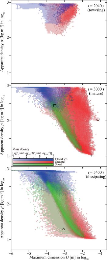
S. Shima et al.: Predicting morphology of ice particles using the super-droplet method                                              4111

2.5   Porous spheroid approximation of ice particles                   3     Variables for moist air

Ice particles have diverse morphologies such as columns,               We only consider dry air and water vapor for the gas phase
hexagonal plates, dendrites, rimed crystals, graupel, hail-            and ignore other trace gases. In this section, we introduce
stones, and aggregates (e.g., Magono and Lee, 1966; Kikuchi            several variables that describe the state of moist air: wind
et al., 2013). Following the strategies of Chen and Lamb               velocity U = (U, V , W ), density of dry air ρd , density of
(1994a, b), Misumi et al. (2010), and Jensen and Harring-              water vapor ρv , density of moist air ρ := ρd + ρv , specific
ton (2015), let us approximate each ice particle as a porous           humidity qv := ρv /ρ, mass of dry air per unit mass of
spheroid, which is characterized by three variables, namely            moist air qd := ρd /ρ, temperature T , pressure P , and po-
equatorial radius a, polar radius c, and apparent density ρ i .        tential temperature of moist air θ := T /5 := T /(P /P0 )R/cp .
That is, the ice particle’s apparent volume is V = (4π/3)a 2 c,        Here, P0 = 1000 hPa is a reference pressure; Rd , Rv , and
and its mass can be evaluated as m = ρ i V . The two radii a           R := qd Rd + qv Rv are the gas constants of dry air, water
and c represent the ice particle’s spatial extent and ρ i rep-         vapor, and moist air, respectively; and cpd , cpv , and cp :=
resents its internal structure. Let us define the aspect ratio         qd cpd + qv cpv are the isobaric specific heats of dry air, wa-
as φ := c/a. A spheroid is considered a prolate spheroid               ter vapor, and moist air, respectively. To simplify notation,
if φ > 1, and columns could be approximated by prolate                 we introduce a variable representing the state of moist air:
spheroids. In contrast, plates and dendrites are approximated          G := {U , ρ, qv , θ, P , T }.
by oblate spheroids, i.e., φ < 1. If an ice particle is hollowed
out or intricately branched, ρ i becomes smaller than the ice
                         i
crystal’s true density ρtrue ≈ 916.8 kg m−3 .                          4     Time evolution equations of mixed-phase clouds

2.6   Rime mass and number of monomers                                 In this section, we describe our model’s time evolution equa-
                                                                       tions, first from cloud microphysics and then moist air fluid
Following Brdar and Seifert (2018) we introduce two addi-              dynamics. Our model is detailed; however, it still falls short
tional ice particle attributes, namely rime mass mrime and             in completely describing mixed-phase cloud microphysics.
number of monomers nmono . Rime mass mrime records the                 To keep the model description concise, discussions on the
mass of ice a particle has obtained through the riming pro-            shortcomings and how to overcome them are left for Sect. 9.
cess. The number of monomers nmono is an integer repre-
senting the number of primary ice crystals in the particle. In         4.1     Cloud microphysics
this study, mrime and nmono are used only for analyzing the
simulation results. Unlike the McSnow model of Brdar and               Let us assign a unique index i to each particle. This
Seifert (2018), this study’s time evolution equations do not           section explains the time evolution equations of particles
depend on mrime or nmono , as will be detailed in Sect. 4.1.                                                  wp          wp
                                                                       {{x i (t), a i (t)}, i = 1, 2, . . ., Nr }. Here, Nr represents the
                                                                       total number of particles accumulated over the whole period.
2.7   Velocity                                                         However, because of coalescence, precipitation, and other
                                                                       processes, some particles might not exist all the time; thus,
We approximate that each particle is always moving at its
                                                                       we let Ir (t) be the set of particle indices existing in the do-
terminal velocity. Therefore, a particle’s velocity v is a diag-
                                                                       main at time t.
nostic attribute.
                                                                       4.1.1    Advection and sedimentation
2.8   Effective number of attributes

In summary, particle attributes consist of a =                         Particle i’s motion equation is
{r, {msol     insol   fz       i   rime , nmono , v}. We need the
       α }, {mβ }, T , a, c, ρ , m                                     d                                    dx i
                                                                                        drg
mass of insoluble substances {minsol  β , β = 1, 2, . . ., N
                                                             insol }      (mi v i ) = F i − mi g ẑ,             = vi ,               (2)
                                                                       dt                                    dt
(and corresponding INAS densities) to specify freezing
temperature T fz . However, as described in Sect. 4.1, time                                                     drg
                                                                       where mi is the particle’s mass, F i is the force of drag from
evolution equations do not depend on {minsol  β }. Rime mass           moist air, g is Earth’s gravity, and ẑ is the unit vector in the
m rime and the number of monomers n      mono do not affect time                                       drg
                                                                       z-axis direction. Note that −F i gives the reaction force act-
evolution either. Particle velocity v is a diagnostic attribute.       ing on moist air. The momentum of moist air changes as de-
Therefore, the attributes directly relevant to time evolution          scribed in Eqs. (73) and (81).
are reduced to {r, {msol       fz         i
                         α }, T , a, c, ρ }. Compared to the              If terminal velocity is reached, the motion equation be-
warm cloud SDM model of Shima et al. (2009), we have                   comes
introduced four new attributes.
                                                                                              dx i
                                                                       v i = U i − ẑvi∞ ,         = vi ,                             (3)
                                                                                               dt

https://doi.org/10.5194/gmd-13-4107-2020                                                     Geosci. Model Dev., 13, 4107–4157, 2020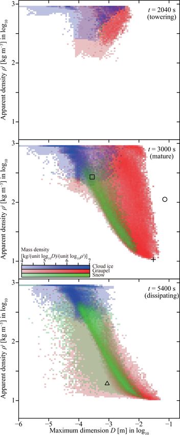
4112                                 S. Shima et al.: Predicting morphology of ice particles using the super-droplet method

where U i := U (x i ) is the ith particle’s ambient wind veloc-         In our model, we assume that ice particles are falling
ity, and vi∞ is the terminal velocity, which is a function of        with their maximum dimension perpendicular to the flow
attributes a i and the state of the ambient air Gi .                 direction. Therefore, the circumcircle area becomes Acc    i =
   In this study, we assume that terminal velocity is always         πmax(ai , ci )2 . The projected area Ai can be roughly eval-
achieved instantaneously; however, this is a simplification.         uated by the area of the circumscribed ellipse Ace         i =
For example, the relaxation time of large droplets is a few          π ai max(ai , ci ); however, we must subtract pores and inden-
seconds (Fig. 3 of Wang and Pruppacher, 1977) though that            tations at boundaries from Ace   i . We assume that the ratio
of micrometer-sized droplets is approximately 10−5 s (see,           Ai /Ace
                                                                           i is a  power   of the volume  fraction ρii /ρtrue
                                                                                                                         i , and that

e.g., Eq. 1 of Chen et al., 2018, and the discussion that fol-       the exponent κ is a function of the aspect ratio φi :
lows). The acceleration of particles can be considered by ex-                            !κ(φi )
plicitly solving the motion equation (see, e.g., Naumann and                      ρii
Seifert, 2015), but extremely small time steps would be re-          Ai = Ace
                                                                           i      i
                                                                                                   .                               (5)
                                                                                 ρtrue
quired for small particles.
   The next two subsections explain the formulas used to cal-        Based on the following arguments, we propose a value κ of
culate droplet and ice particle terminal velocities.                 the form
4.1.2   Droplet terminal velocity                                    κ(φi ) = exp(−φi ).                                           (6)
To calculate droplet terminal velocity, we use the formula               Following Jensen and Harrington (2015), we assume κ →
of Beard (1976): vi∞ = vBeard ∞ (min(r , 3.5 mm); ρ , P , T ),
                                         i             i   i i       1 as φi → 0, and κ → 0 as φi → ∞. φi  1 means that the
where ρi := ρ(x i ) and Pi := P (x i ) are the density and pres-     ice particle is thin and extends horizontally. Therefore, we
sure of ambient moist air, respectively. This formula applies        can expect that the structure is uniform along the vertical
to droplets with radii smaller than 3.5 mm. If we use the for-       axis and that the ratio Ai /Acei is equal to the volume fraction
mula for droplets larger than this, the fall speed becomes un-       ρii /ρtrue
                                                                           i . Thus, κ(φ = 0) = 1. At the other extreme, φ  1
                                                                                           i                                     i
realistically fast. Therefore, we use the fall speed of a droplet    indicates that the ice particle is columnar. Such ice crys-
with a 3.5 mm radius for droplets larger than the size limit.        tals typically hollow inward along their basal face; therefore,
                                                                     the volume fraction ρii /ρtrue
                                                                                                 i   will not affect the ratio Ai /Ace
                                                                                                                                    i .
4.1.3   Ice particle terminal velocity                               Thus, κ(φi → ∞) = 0.
                                                                         For φi ≈ 1, Jensen and Harrington (2015) argued that
For ice particle terminal velocity, we use the
                                                                     (ρii /ρtrue
                                                                             i )κ = 1, i.e., κ = 0. However, this cannot be justified
formula of Böhm (1989, 1992c, 1999): vi∞ =
  ∞ (m , φ , d , q ; ρ , T ), where d is the characteris-            for aggregates with low apparent densities. Thus, we estimate
vBöhm      i i i i i i                    i
                                                                     κ through a dimensional analysis. We assume that the power
tic length, and qi is the area ratio.                                               β               β/s
                                                                     laws mi ∝ Di and Ai ∝ Di hold. Thus, by the definition
   In Böhm’s theory, di is defined by 2ai , and qi is defined by                                                            β−3
the area ratio regarding circumscribed ellipse qice := Ai /Ace       of apparent density, ρii = mi /((4/3)π ai2 ci ) ∝ Di . From
                                                              i ,                 β/s          (β−3)κ
where Ai is the projected area perpendicular to the flow di-         Eq. (5), Di = Di2 Di             . Hence, κ = (2s − β)/{s(3 −
rection, and Acei is the area of the circumscribed ellipse of Ai ,   β)} holds. Schmitt and Heymsfield (2010) estimated that
i.e., the area of the smallest ellipse that completely contains      (β, s) = (2.22, 1.30) for aggregates observed during the Cir-
Ai .                                                                 rus Regional Study of Tropical Anvils and Cirrus Layers
   However, in this study, we start from a slightly different        – Florida Area Cirrus Experiment (CRYSTAL-FACE) field
definition of di and qi , which we adopted mistakenly:               project. Therefore, κ = 0.375 for CRYSTAL-FACE aggre-
                                                                     gates. They also estimated that (β, s) = (2.20, 1.25) for ag-
di = Di := 2max(ai , ci ),    qi = qicc := Ai /Acc
                                                i ,           (4)    gregates observed during an Atmospheric Radiation Mea-
                                                                     surement (ARM) field project, which results in κ = 0.300.
where Di is the maximum dimension, qicc is the area ratio                The κ given by Eq. (6) yields κ(0) = 1, κ(1) = 0.368, and
regarding circumcircle, and Acc   i is the area of the circumcir-    κ(∞) = 0, which agree with the aforementioned estimation.
cle of Ai , i.e., the area of the smallest circle that completely
contains Ai .                                                        4.1.4   Immersion/condensation and homogeneous
   Consequently, Eq. (4) underestimates the fall speeds of                   freezing
columnar ice particles. Nevertheless, based on the assess-
ment detailed in Sect. 9.2, we will confirm that this difference     As explained in Sect. 2.4, a supercooled droplet freezes when
does not change the results of our simulation significantly,         the ambient temperature drops below its freezing temper-
and hence we conclude that this flaw causes only a minor             ature. This section provides a more precise description of
impact on this study. We also note that in Sect. 9.2 we will         when and how freezing occurs in our model.
develop and release a fixed version of the model, SCALE-                We consider that the ith particle freezes immediately when
SDM 0.2.5-2.2.2.                                                     the following three conditions are all satisfied: (1) the parti-

Geosci. Model Dev., 13, 4107–4157, 2020                                                  https://doi.org/10.5194/gmd-13-4107-2020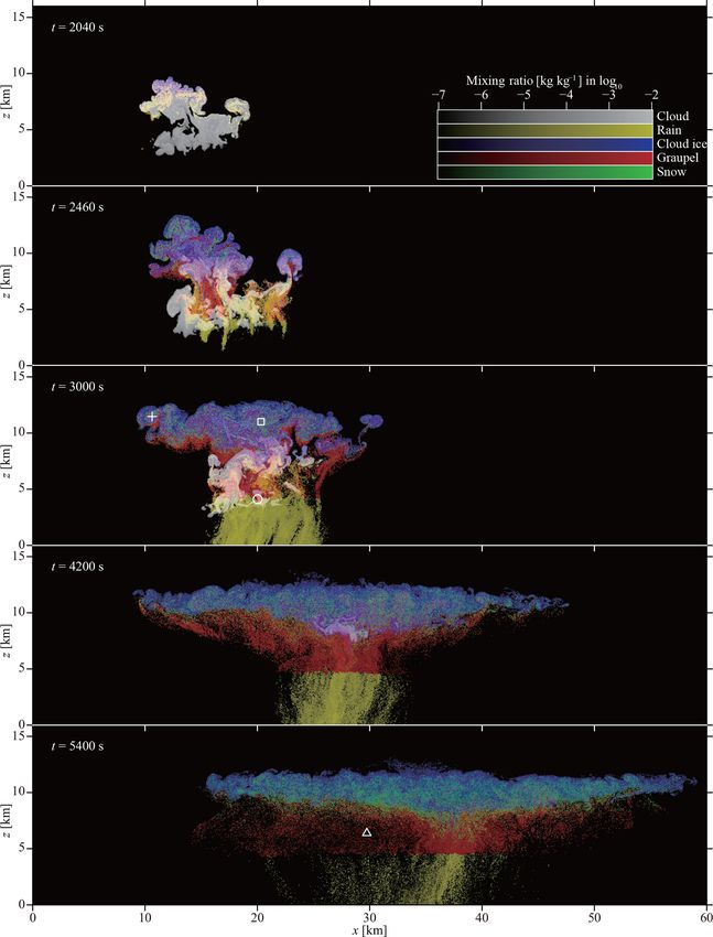
S. Shima et al.: Predicting morphology of ice particles using the super-droplet method                                                 4113

cle is a droplet, i.e., ri > 0; (2) the ambient water vapor is su-       vapor pressure regarding the ith droplet’s surface. Following
persaturated over liquid water, i.e., ei > esw (Ti ); and (3) the        Köhler’s theory (Köhler, 1936), an approximate formula of
                                                                           w,eff
ambient temperature is lower than the particle’s freezing tem-           esi     can be derived as
perature, i.e., Ti < Tifz . Here, ei := e(x i ) and Ti := T (x i ) are      w,eff
                                                                                         a(Ti ) b msol

the ambient vapor pressure and temperature of the ith parti-              esi                             αi
                                                                                   = 1 +        −              ,                   (10)
cle, respectively, and esw (T ) is the saturation vapor pressure         esw (Ti )          ri         ri3
over a planar liquid water surface at temperature T .
                                                                         where a ≈ 3.3×10⁻⁵ cm K/Ti , b ≈ 4.3 cm3 α Iα msol         sol
                                                                                                                      P
    We assume that the resulting ice crystal is spherical, with                                                               αi /Mα ,
                                      i . Therefore, attributes are      Iα is the van ’t Hoff factor, which represents the degree of
the true ice crystal density ρtrue
                                                      i )1/3 , ρ i0 =    ionic dissociation, and Mαsol is the molecular weight of the
initiated as follows: ri = 0, ai = ci0 = ri (ρ w /ρtrue
                           0        0
                                                                  i
  i      mono0               rime0                                       solute α. The second and third terms of Eq. (10) account for
ρtrue , ni     = 1, and mi         = 0. The primed variables here
                                                                         curvature and solute effects, respectively.
denote values after the update, and ρ w is the density of liquid
                                                                             The growth of a droplet by condensation/evaporation is
water. {msol        insol          fz
           αi }, {mβi }, and Ti remain unchanged.                        governed by Eqs. (8)–(10) in our model. When a droplet or
    When freezing occurs, each particle releases latent heat
                                                                         an ice particle falls through the air, the flow around it en-
of fusion to the moist air, as described in Eqs. (74), (79),
                                                                         hances the diffusional growth, a phenomenon known as the
and (80).
                                                                         ventilation effect. It does not essentially affect the growth
4.1.5   Melting                                                          of droplets smaller than 50 µm in radius (see Sect. 13.2.3 of
                                                                         Pruppacher and Klett, 1997). Therefore, for simplicity, we do
When ambient temperature rises above 0 ◦ C, we consider                  not consider the ventilation effect on droplets in this study.
that melting occurs immediately. Thus, the attributes are up-            Notably, Eqs. (8)–(10) also describe the respective activation
dated as follows: ri0 = (ai2 ci ρii /ρ w )1/3 and ai0 = ci0 = ρii0 =     and deactivation of cloud droplets from and to aerosol par-
nmono0 = mrime0 = 0. {msol           insol         fz                    ticles (see, e.g., Arabas and Shima, 2017; Hoffmann, 2017;
  i         i            αi }, {mβi }, and Ti remain un-
changed. When melting occurs, each particle absorbs latent               Abade et al., 2018).
heat of fusion from the moist air, as indicated in Eqs. (74),                Vapor and latent heat couplings to moist air through con-
(79), and (80).                                                          densation and evaporation are calculated by Eqs. (71), (72),
                                                                         (74), (76), (77), and (79).
4.1.6   Condensation and evaporation
                                                                         4.1.7   Deposition and sublimation
Following, e.g., Rogers and Yau (1989), the time evo-
lution equation describing droplet growth by condensa-                   The shapes of ice crystals formed by depositional growth ex-
tion/evaporation can be derived as follows.                              hibit strong dependencies on temperature and, to a lesser ex-
   The growth rate is identical to vapor flux at the droplet             tent, supersaturation (e.g., Nakaya, 1954; Hallett and Mason,
surface. If the diffusion of vapor around the droplet is in a            1958; Kobayashi, 1961). The former is known as the primary
quasi-steady state, we obtain                                            growth habit and the latter as the secondary growth habit. The
                                                                         primary growth habit determines the preferred growth direc-
dmi                    sfc                                               tion, i.e., columnar or planar, and the secondary growth habit
    = 4π ri Dv (ρvi − ρvi  ).                                     (7)
 dt                                                                      determines the mode of growth, i.e., whether the columnar
Here, Dv is water vapor’s diffusivity in air, ρvi := ρv (x i ) is        crystal becomes solid or hollow, and whether the planar crys-
                                                   sfc is water
the ambient moist air’s water vapor density, and ρvi                     tal becomes plate-like, sectored, or dendritic. In this study,
vapor density at the surface of the droplet.                             we use the model of Chen and Lamb (1994a) with various
   If we further assume that thermal diffusion is also in a              modifications.
quasi-steady state, and that surface temperature Tisfc and am-              The mass growth rate can be derived similarly to Eqs. (7)
bient temperature Ti are close to each other, i.e., (Tisfc −             and (8):
Ti )/Ti  1, Eq. (7) can be reduced to                                   dmi                                   Si − 1
                                                                                              sfc
                                                                             = 4π CDv (ρvi − ρvi  )fvnt = 4π C ii      fvnt ,           (11)
                                                                                                              Fk + Fdi
                         (          w,eff
                                          )
   dri          1                 e                                       dt
ri     = w w               S w − wsi        ,                (8)
   dt    ρ (Fk + Fdw ) i         es (Ti )                                where Sii := ei /esi (Ti ) is the ambient saturation ratio over ice,
                                                                         and esi (T ) is the saturation vapor pressure over ice at temper-
where Siw := ei /esw (Ti ) is the ambient saturation ratio over
                                                                         ature T ,
liquid water, and
                                                                                    Ls          Ls               Rv Ti

          Lv

                      Lv               Rv Ti                             Fki =            −1         , Fdi =                ,           (12)
  w
Fk =           −1         , Fdw =                ,          (9)                   Rv Ti         kTi            Dv esi (Ti )
         Rv Ti        kTi           Dv esw (Ti )
                                                                         where Ls is the latent heat of sublimation, C = C(ai , ci )
where Lv is the latent heat of vaporization, k is the thermal            is the electric capacitance of the spheroid, and fvnt is the
                                w,eff
conductivity of moist air, and esi    is the effective saturation        particle-averaged ventilation coefficient.

https://doi.org/10.5194/gmd-13-4107-2020                                                    Geosci. Model Dev., 13, 4107–4157, 2020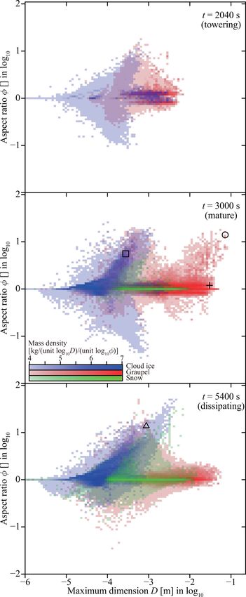
4114                                 S. Shima et al.: Predicting morphology of ice particles using the super-droplet method

   The exact form of capacitance C(ai , ci ) is given by Chen        because of the air flow around it. Chen and Lamb (1994a)
and Lamb (1994a). C ≈ (2ai + ci )/3 gives a good approxi-            derived a fvnt of the form
mation for φi ≈ 1.
   The coefficient fvnt accounts for the ventilation effect, i.e.,            b1 + b2 X γ (ci /C)1/2
                                                                     fvnt =                               .                     (17)
the enhancement of diffusional growth by air flow. Hall and                   b1 + b2 X γ (ai /C)1/2
Pruppacher (1976) suggested that fvnt could be described by
                                                                        The secondary growth habit is expressed by deposition
fvnt = b1 + b2 X γ ,                                         (13)    density ρdep , which represents the apparent density of the ice
                                                                     fraction newly created by deposition. Then, the change in ice
where (b1 , b2 , γ ) = (1.0, 0.14, 2) for X ≤ 1, (b1 , b2 , γ ) =    particle volume dVi is given by
                                                 1/3    i )1/2 ,
(0.86, 0.28, 1)       for      X > 1,     X = NSc (NRei
                                              i
NSc = µ/(ρDv ) is the Schmidt number, NRei = ρvi Di /µ  ∞                     dmi
                                                                     dVi =         ,     for dmi ≥ 0 (deposition).              (18)
is the Reynolds number of ice particle i, and µ is the                        ρdep
dynamic viscosity of moist air.
                                                                     Deposition density ρdep can be expressed as
   Note that mi in Eq. (11) can become zero through subli-
mation over a finite time. However, in this study, we prohibit             (
                                                                             ρi ,        for 0(Ti ) < 1 ∧ ai < 100 µm;
complete sublimation, and instead, we impose a limiter to            ρdep = true
                                                                               CL94
                                                                                                                                (19)
dmi as follows:                                                              ρdep ,      otherwise.

dmi = max(dmi , mimin − mi ),                                (14)    Here, following Jensen and Harrington (2015), we assume
                                                                     that planar crystal branching does not occur if the equato-
                                                                                                              CL94
where mimin is an arbitrary small mass taken from the mass of        rial radius ai is smaller than 100 µm. ρdep   is an empirical
a spherical ice particle with a radius of 1 nm and the true ice      formula of deposition density proposed by Chen and Lamb
           i . This is a crude representation of pre-activation
density ρtrue                                                        (1994a),
(see, e.g., Marcolli, 2017, for a review). Each particle keeps
                                                                                           3max(1ρi − 0.05 g m−3 , 0)

the memory of ice activation until the ambient temperature             CL94
                                                                     ρdep       i
                                                                            = ρtrue exp −                                ,   (20)
rises above 0 ◦ C. A particle with mimin ice grows immediately                                     0(Ti ) g m−3
after the ambient air is supersaturated over ice, irrespective of
                                                                                         sfc . From Eq. (11), 1ρ becomes
                                                                     where 1ρi := ρvi − ρvi
its freezing temperature Tifz .                                                                                 i
   In Chen and Lamb’s (1994a) model, the primary growth
habit is expressed by an empirical function known as the in-                        Sii − 1
                                                                     1ρi =                       .                              (21)
herent growth ratio 0(T ), which modulates the c-axis to a-                   Dv (Fki + Fdi )
axis growth rate ratio:
                                                                     Here, following Miller and Young (1979), we limit ρvi by
dci             ci     ci                                            water saturation and replace the 1ρi in Eq. (20) with
    = 0(Ti )fvnt =: 0 ∗ ,                                    (15)
dai             ai     ai
                                                                                    min(Sii , esw (Ti )/esi (Ti )) − 1
where fvnt is the primary growth habit’s ventilation coeffi-         (1ρi )↓ =                                           .      (22)
                                                                                              Dv (Fki + Fdi )
cient, and 0 ∗ is the effective inherent growth ratio, including
the ventilation effect.                                                For sublimation, the particle volume change dVi is given
   For purely diffusional growth, dci /dai = ci /ai holds;           by
therefore, the aspect ratio does not change, i.e., dφi = 0.
0(T ) represents the lateral redistribution of vapor on the                   dmi
                                                                     dVi =         ,     for dmi < 0 (sublimation),             (23)
ice crystal surface through kinetic processes. We use the                     ρsbl
0(T ) proposed by Chen and Lamb (1994a) but set 0(T ) =
                                                                     where sublimation density ρsbl represents the apparent den-
1 for D < 10 µm, as observations suggest that ice crystals
                                                                     sity of the ice fraction removed by sublimation. For simplic-
are quasi-spherical if D < 60 µm (Baran, 2012; Korolev and
                                                                     ity, we assume that the ice particle’s apparent density will not
Isaac, 2003; Lawson et al., 2008). Additionally, the 0(T )
                                                                     be changed through sublimation, i.e.,
provided in Chen and Lamb (1994a) is for temperatures be-
tween −30 and 0 ◦ C. For lower temperatures, we simply as-           ρsbl = ρii .                                               (24)
sume
                                                                       We can now calculate the attributes at time t + dt. The ap-
0(T ) = 0(−30 ◦ C) ≈ 1.28,       for T < −30 ◦ C.            (16)    parent density becomes
  The ventilation coefficient fvnt represents the preferential                         mi + dmi
enhancement of vapor flux toward the ice crystal’s major axis        ρii (t + dt) =             ,                               (25)
                                                                                       Vi + dVi

Geosci. Model Dev., 13, 4107–4157, 2020                                                   https://doi.org/10.5194/gmd-13-4107-2020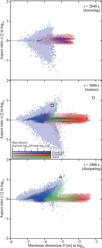
S. Shima et al.: Predicting morphology of ice particles using the super-droplet method 4115
where dmi is given in Eqs. (11) and (14), and dVi is given in Shima et al., 2009; Dziekan and Pawlowska, 2017). Then,
Eqs. (18) and (23). all particle pairs in the volume can collide and coa-
From Eq. (15) and the definition of volume Vi = lesce/rime/aggregate during an infinitesimal time interval dt.
(4π/3)ai2 ci , after dt, the two radii become The probability that a particle pair j and k inside 1V will
collide and coalesce/rime/aggregate within an infinitesimal
d log Vi time interval (t, t + dt) is given by
ai (t + dt) = ai exp , (26)
2 + 0∗ dt
∗
0 d log Vi
Pj k = K(a j , a k ; G) , (31)
ci (t + dt) = ci exp . (27) 1V
2 + 0∗
where the function K(a j , a k ; G) is called the collision–
Applying those equations to a small ice particle’s sublima- coalescence/–riming/–aggregation kernel, and G denotes the
tion creates an extremely small planar or columnar ice parti- state of the moist air in 1V .
cle. However, observations suggest that ice crystals are quasi- In this study, we consider coalescence, riming, and aggre-
spherical if D < 60 µm (Baran, 2012; Korolev and Isaac, gation induced by differential gravitational settling of par-
2003; Lawson et al., 2008). Therefore, we regard the ice par- ticles because this mechanism is dominant in mixed-phase
ticle as spherical with the true ice density if the minor axis clouds.
predicted by Eqs. (26) and (27) is smaller than 1 µm. That is,
4.1.9 Coalescence between two droplets
if min{ai (t + dt), ci (t + dt)} < 1 µm,
First, we consider droplet coalescence, which accounts for
ρii0 (t + dt) = ρtrue
i
, (28)
the formation of rain droplets from cloud droplets (autocon-
!1
mi + dmi 3 version), the collection of cloud droplets by rain droplets
ai0 (t + dt) = ci0 (t + dt) = , (29) (accretion), and the coalescence of two rain droplets (self-
(4π/3)ρii0 (t + dt)
collection).
where primed variables indicate values after correction. The collision–coalescence kernel is given by
For simplicity, we assume that the rime mass fraction Kcoal = Ecoal (rj , rk )π(rj + rk )2 |vj∞ − vk∞ |, (32)
mrime
i /mi does not change through sublimation, following
Brdar and Seifert (2018): where Ecoal (rj , rk ) is the collection efficiency of collision–
coalescence, which can be decomposed into Ecoal =
collis E coal . Here, collision efficiency E collis considers the
mrime
i , for dmi ≥ 0; Ecoal coal coal
rime effect that a smaller droplet is swept aside by the flow around
mi (t + dt) = m i + dm i (30)
mrime
i , for dmi < 0. a larger droplet, or a droplet being caught in the wake of a
mi
similarly sized droplet collides on the downstream side. We
Vapor and latent heat couplings to moist air through depo- adopt the collision efficiency used in Seeßelberg et al. (1996)
sition and sublimation are calculated by Eqs. (71), (72), (74), and Bott (1998). Here, Davis (1972) and Jonas (1972) are
(76), (78), and (79). used for small droplets, and Hall (1980) for larger droplets,
In this section, we detailed the deposition and sublimation with modifications to the collector droplet radius range 70–
model used in SCALE-SDM; however, there is significant 300 µm to incorporate the wake effect suggested by Lin and
room for improvement. For example, as we will discuss in Lee (1975). Not all the collisions end up with coalescence.
Sect. 9.1.4, using 0(T ) for sublimation is questionable. In- Rebound or breakup (fragmentation) could also occur. Coa-
stead, we propose using 0(T ) = 1 for sublimation (Eq. 110), lescence efficiency Ecoal coal represents the fraction of collisions
and validate this correction in Sect. 9.1.5. Furthermore, in that result in permanent coalescence. In this study, we as-
Sect. 9.2, to prohibit the creation of unnaturally slender ice sume Ecoalcoal = 1 for simplicity.
particles, we will propose to impose a limiter to the effective If coalescence takes place, droplets j and k then merge
inherent growth ratio 0 ∗ (Eq. 123). Several other issues of into a single droplet. Thus, we keep j and remove k from the
our deposition/sublimation model, such as the representation system. The attributes of the new droplet j can be calculated
of polycrystals, will be discussed in Sect. 9.3.5. as follows:
1
4.1.8 Stochastic description of coalescence, riming, and rj0 = (rj3 + rk3 ) 3 , (33)
aggregation msol0 sol sol sol
αj = mαj + mαk , α = 1, 2, . . ., N (34)
Particle coalescence, riming, and aggregation can be con- minsol0
βj = minsol
βj + mβk ,
insol
β = 1, 2, . . ., N insol
(35)
sidered a stochastic process. Following Gillespie (1972),
Tjfz0 = max(Tjfz , Tkfz ), (36)
consider a region with volume 1V . If 1V is sufficiently
small, we can consider that particles within this region where primed values indicate the resultant droplet. Here,
are well mixed, e.g., by atmospheric turbulence (see, e.g., we assumed that the resultant particle’s Tjfz0 is given by
https://doi.org/10.5194/gmd-13-4107-2020 Geosci. Model Dev., 13, 4107–4157, 2020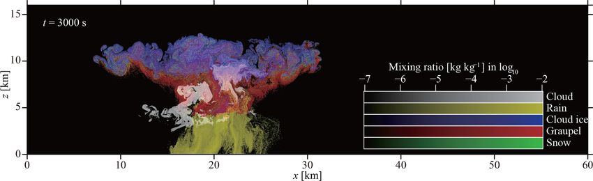
4116                                   S. Shima et al.: Predicting morphology of ice particles using the super-droplet method

max(Tjfz , Tkfz ), i.e., the higher freezing temperature of the      following Hall (1980), Rasmussen and Heymsfield (1985),
two constituent particles. We also assume that the same ap-          and Heymsfield and Pflaum (1985). For columnar and planar
plies to riming and aggregation.                                                                     clm and E pln
                                                                     ice particles, we use formulas EEM17      EM17 from Erfani
   Let us emphasize that the stochastic model introduced in          and Mitchell (2017), which were obtained by fitting the nu-
this section describes the underlying mathematical model of          merical results of Wang and Ji (2000). For the intermediate
the coalescence process, not the Monte Carlo algorithm of            case, we calculate an average weighted by the aspect ratio
SDM that solves the stochastic process numerically. In the           φj . For φj ≤ 1 (planar),
preceding paragraph, droplet k was removed from the system
because both j and k are real particles. On the contrary, in         Erime =φj EBG74 (p w/i , NRej
                                                                                               i
                                                                                                   , NmFr )
the SDM, the number of super-particles is (almost always)                                    pln  i
                                                                               + (1 − φj )EEM17 (NRej , NmFr ).                   (40)
conserved through coalescence (Shima et al., 2009).
                                                                     For φj > 1 (columnar),
4.1.10   Riming between an ice particle and a droplet
                                                                               1
                                                                     Erime =      EBG74 (p w/i , NRej
                                                                                                   i
                                                                                                      , NmFr )
Riming usually refers to the collection of small supercooled                   φj
droplets by a larger ice particle, but we also include the col-
                                                                                       1

                                                                                                clm     clm
lection of small ice particles by a larger droplet. The latter                 + 1−         EEM17    (NRej  , NmFr ).             (41)
                                                                                      φj
case could be regarded as a type of contact freezing. How-
ever, ice particles grow preferentially when ice particles and       Here,          pw/i := 1/p i/w = rk /rji ,        NmFr = (vj∞ −
supercooled droplets coexist (Wegener–Bergeron–Findeisen              ∞     ∞                     clm      ∞
                                                                     vk )vk /(gDj /2), and NRej = ρvj 2aj /µ is the Reynolds
mechanism). Therefore, we can expect that the latter case            number based on the width of column 2aj . Note that there is
happens less frequently in mixed-phase clouds.                       a typo in Eq. (19) of Erfani and Mitchell (2017); i.e., the two
   Hereafter we assume, without loss of generality, that par-        case conditions are opposite.
ticle j is an ice particle and particle k is a droplet. The             If riming takes place, the ice particle j and droplet k merge
collision–riming kernel is expressed as                              and instantaneously freeze into a single ice particle. Thus, we
Krime = Erime Ag |vj∞ − vk∞ |,                               (37)    keep j and remove k from the system.
                                                                        If max(aj , cj ) < rk , we assume that the resultant ice parti-
where Erime is the collision–riming collection efficiency and        cle is spherical with the true ice density:
Ag is the geometric cross-sectional area of j and k.
  Figure 1 of Wang and Ji (2000) defines Ag for riming, but          ρji0 = ρtrue
                                                                              i
                                                                                  ,                                               (42)
calculating it rigorously for porous spheroid models is im-                                     1
                                                                                      mj + mk     3
possible. Thus, we approximate Ag by                                 aj0 = cj0 =            i
                                                                                                    ,                             (43)
                                                                                     (4π/3)ρtrue
Ag = π(aj + rk ){max(aj , cj ) + rk } − (Ace
                                          j − Aj );          (38)
                                                                     mrime0
                                                                      j     = mrime
                                                                               j    + mk ,                                        (44)
i.e., the indentation of the ice particle (Ace
                                             j − Aj )      is sub-
                                                                     nmono0
                                                                      j     = nmono
                                                                               j    ,                                             (45)
tracted from the area of an ellipse with semi-axes (aj + rk )
and {max(aj , cj ) + rk }. Therefore, if rk  aj , cj , then Ag ≈    msol0     sol      sol               sol
                                                                       αj = mαj + mαk , α = 1, 2, . . ., N ,                      (46)
Aj . At the other extreme, if rk  aj , cj , then Ag ≈ π(aj +
                                                                     minsol0
                                                                       βj    = minsol       insol
                                                                                 βj + mβk , β = 1, 2, . . ., N
                                                                                                               insol
                                                                                                                     ,            (47)
rk ){max(aj , cj ) + rk }.
   To evaluate collision–riming collection efficiency Erime ,        Tjfz0 = max(Tjfz , Tkfz ),                                   (48)
we combine formulas proposed by Beard and Grover (1974)
                                                                     where primed values indicate the resultant ice particle.
and Erfani and Mitchell (2017).
                                                                        If max(aj , cj ) ≥ rk , we preserve the ice particle’s max-
   If vj∞ < vk∞ , we consider droplet k as the collector and
                                                                     imum dimension, i.e., Dj0 = Dj , until the ice particle be-
adopt the formula of Beard and Grover (1974):
                                                                     comes quasi-spherical. This accounts for the gradual growth
                                 i/w
Erime = EBG74 (p i/w , NRek
                        w
                            , NSt ),                         (39)    of an unrimed ice crystal to a graupel particle with a quasi-
                                                w = ρv ∞ 2r /µ       spherical shape. This filling-in simplification was introduced
where p i/w := rji /rk , rji := (aj2 cj )1/3 , NRek   k    k
                                                                     by Heymsfield (1982), and is used in various models (e.g.,
                                                            i/w
is the Reynolds number of droplet k, NSt =                           Chen and Lamb, 1994b; Morrison and Grabowski, 2008,
               w C /(9ρ) is the Stokes impaction pa-
(p i/w )2 ρji NRek SC                                                2010; Jensen and Harrington, 2015; Morrison and Milbrandt,
rameter when droplet k is collecting an ice particle, and CSC        2015). As graupels have an aspect ratio of approximately
is the Cunningham slip correction factor.                            0.8 (Heymsfield, 1978), we preserve the minor dimension if
   If vj∞ ≥ vk∞ , we consider ice particle j to be the collec-       0.8 < φj ≤ 1/0.8 = 1.25, which mimics graupel’s tumbling.
tor. For spherical ice particle φj ≈ 1, we again use the for-        When an accreted droplet freezes, the air will be trapped in-
mula of Beard and Grover (1974) but replace the Stokes im-           side. Let rime density ρrime be the frozen droplet’s appar-
                      i/w
paction parameter NSt with the mixed Froude number NmFr              ent density. Then, for φj ≤ 0.8 (planar) and 1.0 < φj ≤ 1.25

Geosci. Model Dev., 13, 4107–4157, 2020                                                 https://doi.org/10.5194/gmd-13-4107-2020
S. Shima et al.: Predicting morphology of ice particles using the super-droplet method 4117
(columnar but quasi-spherical), We propose to replace the Y in Eq. (56) (not in Eq. 57)
with Y ↓ = min(Y, 3.5) (Eq. 107), because the rime density
mj + mk
ρji0 = , (49) derived from Eq. (56) becomes too small for larger values
Vj + mk /ρrime of Y , which affects the shape of hailstones near the freezing
aj0 = aj , (50) level.
Vj + mk /ρrime Another issue discussed in Sect. 9.1.2 is related to the
cj0 = . (51) filling-in model. Assuming that the diameter of the frozen
(4π/3)aj2
droplet is preserved, if the diameter is larger than the ice par-
Other attributes are updated using Eqs. (44)–(48). For ticle’s maximum dimension, we propose replacing Eq. (50)
φj > 1.25 (columnar) and 0.8 < φj ≤ 1.0 (planar but quasi- by Eq. (108) and Eq. (54) by Eq. (109).
spherical), We validate these two corrections in Sect. 9.1.5. More
discussions to refine our riming model will be presented in
mj + mk Sect. 9.3.7.
ρji0 = , (52)
Vj + mk /ρrime
1 4.1.11 Aggregation between two ice particles
0 Vj + mk /ρrime 2
aj = , (53)
(4π/3)cj Finally, we consider the aggregation of ice particles. Fol-
cj0 = cj . (54) lowing Connolly et al. (2012), we use the projected area of
particles to evaluate the geometric cross-sectional area. The
Other attributes are updated using Eqs. (44)–(48). Following collision–aggregation kernel is then given by
Chen and Lamb (1994b), we use the formula of Heymsfield
1 2
1
and Pflaum (1985) to calculate rime density ρrime :
Kagg = Eagg Aj + Ak |vj∞ − vk∞ |,
2 2
(59)
HP85
ρrime = max{min{ρrime (Y ), 0.91 g cm−3 }, 0.1 g cm−3 },
where Eagg is the collision–aggregation collection efficiency.
(55)
Following Morrison and Grabowski (2010), we assume that
where Y := (−rk vimp /Tjsfc )/(µm m s−1 /◦ C), vimp is impact the efficiency is given by a constant, Eagg = 0.1, in this study.
velocity, and Tjsfc is the surface temperature of ice particle j . Field et al. (2006) confirmed that Eagg = 0.09 produces a
good agreement with aircraft observations.
If aggregation takes place, ice particles j and k merge into
a single ice particle. Thus, we keep j and remove k from the
system. However, no reliable model exists for calculating the
next porous spheroid. Chen and Lamb (1994b) proposed a
where A = 0.30 g cm−3 , B1 = 0.44, B2 = −0.03115, B3 = model, but it tends to create snow aggregates with impossibly
−1.7030, B4 = 0.9116, and B5 = −0.1224. low apparent densities (lighter than vapor). In this study, we
Impact velocity can be calculated using the propose another intuitive model by incorporating the com-
formula of Rasmussen and Heymsfield (1985): paction of fluffy snowflakes to cope with the problem.
i , w/i Snow aggregates have complicated fractal structures.
vimp = |vj∞ − vk∞ |max{fRH85 (NRej NSt ), 0}, where
w/i i /(9ρ) is the Stokes impaction pa- However, if we circumscribe them using a spheroid, the
NSt = (p w/i )2 ρ w NRej
growth by aggregation is in three dimensions, rather than one
rameter when an ice particle collects a droplet. Because the
(columnar) or two (planar). Therefore, as in the case of rim-
fRH85 given in Rasmussen and Heymsfield (1985) becomes
w/i ing, we assume that only the minor dimension grows by ag-
slightly negative around 0.1 < NSt < 1.0, we impose a gregation.
limiter to ensure it is positive. Surface temperature Tjsfc can
If the volume-weighted average density ρji k = (mj +
be evaluated as i ,
mk )/(Vj + Vk ) is closer to the true density of ice ρtrue
Ls Dv the two particles aggregate without changing their shapes.
Tjsfc = Tj + 1ρj , (58)
k Hence, when we approximate the resultant aggregate with
where 1ρj is given in Eq. (21). This equation is derived un- a spheroid, there are more empty spaces inside, thus reduc-
der an assumption of quasi-steady vapor and thermal diffu- ing the apparent density. Let us denote the minimum possi-
sion. ble apparent density as ρji,min
k , which can be evaluated using
When riming occurs, the frozen droplet releases the latent Eq. (61), which we will derive shortly.
heat of fusion to the moist air as described in Eqs. (74), (79) In contrast, if ρji k is small, compaction of the fluffy
and (80). snowflakes occurs, and the empty space of the larger ice
As we will discuss in Sect. 9.1.1, the rime density formula particle could be filled with the smaller ice particle or the
of Heymsfield and Pflaum (1985) must be revised slightly. particles might deform because of the collision–aggregation
https://doi.org/10.5194/gmd-13-4107-2020 Geosci. Model Dev., 13, 4107–4157, 2020You can also read


