Prediction of NBA games based on Machine Learning Methods - University of Wisconsin Madison
←
→
Page content transcription
If your browser does not render page correctly, please read the page content below
University of Wisconsin Madison

Prediction of NBA games based on Machine Learning Methods

                The code can be posted on the website

                      Renato Amorim Torres

                        Instructor: Y. H. Hu

                          December, 2013
Introduction
National Basketball Association (NBA ) is the men's professional basketball league in North
America. The influence of NBA trespass its borders and have countless fans around all the world.
As the league involves a lot of money and fans, not surprisingly, a lot of studies have been
developed trying to predict its results, to simulate winning teams, to analyze player's performance
and to assist coaches.
Through the years a lot of data and statistics have been collected based on NBA and each
day the data become more rich and detailed. Although, even with such rich data available, it is still
very complex to analyze and try to predict a game. In order to deal with that complexity and to
achieve better predictions rate a lot of Machine Learning methods have been implemented over
these data. That is exactly the purpose of this project.
The main objective is to achieve a good prediction rate using Machine Learning methods.
The prediction will only define the winning team, regardless of the score. As a parameter and as a
goal, our prediction rate should be higher than the rate of the very naive majority vote classifier that
always looked at all previous games (in the season) between two teams and picked the one with the
fewest losses as the winner. Moreover, it would be interesting to discover not only the winner, but
also what are the most important features to be one. Finally, as a secondary objective, we will try to
classify the position of one player based on his features.
Background (NBA format)
(nfIormation from http://en.wikipedia.org)
The current league organization divides thirty teams into two conferences of three divisions
with five teams each.
Eastern Conference Western Conference
Atlantic Central Southeast Northwest Pacific Southwest
5 teams 5 teams 5 teams 5 teams 5 teams 5 teams
During the regular season, each team plays 82 games, 41 at home and 41 away. A team faces
opponents in its own division four times a year (16 games). Each team plays six of the teams from
the other two divisions in its conference four times (24 games), and the remaining four teams three
times (12 games). Finally, each team plays all the teams in the other conference twice apiece (30
games).
NBA Playoffs begin in late April, with eight teams in each conference going for the
Championship. The three division winners, along with the team with the next best record from the
conference are given the top four seeds. The next four teams in terms of record are given the lower
four seeds.
The playoffs follow a tournament format. Each team plays an opponent in a best-of-seven
series, with the first team to win four games advancing into the next round, while the other team is
eliminated from the playoffs. In the next round, the successful team plays against another advancing
team of the same conference. All but one team in each conference are eliminated from the playoffs.
The final playoff round, a best-of-seven series between the victors of both conferences, is
known as the NBA Finals, and is held annually in June.Methodology
Firstly, the data-set should be studied, selected and organized. It is important to mention that
only the Regular Season data will be used, once not all teams plays in playoffs and also the teams
that plays it can changes from one year to another.
Although there are a lot of rich data available, a lot of time it is not ready to be used.
Sometimes it is desirable to select the most important features or also to reduce its number using
methods as Principal Components Analysis. After the data is prepared some analysis will be done in
order to select the best inputs for the methods.
Secondly, the Machine Learning Methods will be implemented. By looking in some articles
cited on the references, it seems interesting to start the process with a linear regression, that
represents a simple method that has, so far, achieved a good performance. After tried the linear
regression and, hopefully, with a good classification rate another method will be explored trying to
achieve a better performance. Comparing two methods the results will be more reliable and it will
be easier to detect the most important features and to find possible improvements. During the
process, probably many modifications will be necessary, so new data analysis may be necessary and
also new data preparation.
Obs.: This methodology is a guide, but other methods can be tested and implemented if achieves
better results.
Data Preparation
Data Extraction
To decide the data source many websites were visited: Most part of the websites has a wide
range of data that goes from the basic box score even to the player's salary. Some points were
essential in deciding the data source: first, the easiness of extracting the data from the website;
second, the number of seasons provided by the website and finally the basic prerequisites of any
data as reliability and utility.
The website http://www.basketball-reference.com presented all these features and was
selected as major source. The boxscores in the website is organized in tables as shown below:
To extract the data, the box scores were copied into spreadsheets of the OpenOffice and,
using the tool macro, all the team names were replaced by numbers, the unnecessary columns were
deleted, and .txt files were generated with the data. The .txt files generated were loaded in MatLab
and used to generate the feature vectors.
The data extracted was from only regular seasons from the 2006-2007 season to 2012-2013
season. Just for simplicity, now and then the season will only be referred by the year that it started.
(so 2012-2013 season will be referred 2012 season). During the data extraction it was observedsome irregularities: the regular season 2012-2013 has only 1229 games and the regular season
2011-2012 has only 990 games, also some teams change its names through the period of 2006-2013.
The website, also contains some League Standings as displayed below:
Some of the these standings were used during the project, however they were not extracted
directly from the website, but, instead, they were derived from the box scores using MatLab scripts.
This approach was easier than developing a code as phyton to extract the information from the
website. Anyway, the standings of the website were very useful to verify the correctness of the
MatLab scripts comparing some standings samples obtained with the website.
Feature Vectors Implementation / Data Anaysis
It is really important to spend some time deciding what are going to be the features vectors
(input) of the methods, otherwise the results will be frustrating. This fact is well summarized in the
phrase "Garbage in, garbage out" , very common in the field of computer science
Initially, the most intuitive features were implemented as the Win-Loss percentage of both
teams and point differential per game of both teams. Posteriorly some other features as: Visitor
Team win-Loss percentage as visitor, Home Team win-Loss percentage at home and win-loss
percentage in the previous 8 games for both teams. All these features were analyzed through some
charts or making some simple predictions.
The table below presents the predictions results obtained using:
A: Win-Loss Percentage of both teams in all previous games of the season and choosing the one
with highest percentage as the winning team.
B: point differential per game of both teams in all previous games of the season and choosing the
one with highest point differential as the winning team.
C: win-loss percentage of both teams in the previous 8 games and choosing the one with highest
percentage as the winning team.
D: Visitor Team win-Loss percentage as visitor and Home Team win-Loss percentage at home in all
previous games and chosing the one with highest percentage as the winning team.
E: Prediction based on the results of previous games between those teams. The team with more
wins is predicted as the winner.Data Analysis
Regular Season A B C D E
2006 0.6077 0.5972 0.5772 0.6252 0.5358
2007 0.6524 0.6650 0.6411 0.6711 0.5782
2008 0.6524 0.6650 0.6411 0.6711 0.5782
2009 0.6370 0.6398 0.5931 0.6581 0.5835
2010 0.6516 0.6565 0.6285 0.6606 0.5818
2011 0.6308 0.6263 0.6076 0.6434 0.6055
2012 0.6469 0.6603 0.6168 0.6452 0.5921
Mean 0.6398 0.6443 0.6150 0.6536 0.5793
Observations:
- Sometimes, the prediction is impossible because there is no information yet about the
teams (very common in the first games of the season) or because the percentages of both teams are
equal, or the team have not played 8 games yet. When it occurs, the number of unpredictable games
is computed and at the end it is considered that half of them was correctly predicted (according to
the probability).
-In the prediction C, it was used the percentage of both teams in the previous 8 games. The
aim of this feature is analyze the performance of the team in a short period of time. The number 8
was selected after analyzing the prediction rate for N numbers of previous games for N from 1 to
10. When N=8, it achieved the highest prediction rate.
- Another analysis done was to verify how the prediction rate increases as more data from
the season is collected. It can be observed in the graph below that in the first seven games the
prediction increases much faster.-Through the results above it can be observed that all the features are well related with the
predction of the game and are good candidates as input for the methods.
- All the features has information of the current season only. None of them uses, for
example, the percentage of win-loss of the team in the previous season. It means that the data of
previous years are used only to train the methods, but not as a data for the current season.
Methods
Primarily, lets remember our goal: "As a parameter and as a goal, our prediction rate should
be higher than the rate of the very naive majority vote classifier that always looked at all previous
games (in the season) between two teams and picked the one with the fewest losses as the winner”.
Therefore we are going to define our minimum prediction rate. Although, instead of using the the
number of losses we are going to use the win-loss percentage, as the number of games played by
one team, in a specific day of the season, can differ from the number played by the opponent.
This parameter has already been calculated during the data analysis and corresponds to the
data analysis A from the table. So our goal is to have predictions rates better than:
Very naive majority vote classifier
Regular Season Prediction Rate
2006 0.6077
2007 0.6524
2008 0.6524
2009 0.6370
2010 0.6516
2011 0.6308
2012 0.6469
Mean 0.6398Linnear Regression
The first method implemented was the linnear regression. The method consists in multiply
each feature by a weight, make a summation of all values obtained and a bias, and use this final
value to do the classification.
In our case, if Y > 0, the visitor team is considered winner and if Y < 0 the home team is
considered winner. Initially all the features obtained were applied as input of the linnear regression:
1. Win-Loss Percentage (Visitor Team)
2. Win-Loss Percentage (Home Team)
3. Point differential per game (Visitor Team)
4. Point differential per game (Home Team)
5. Win-loss percentage previous 8 games (Visitor Team)
6. Win-loss percentage previous 8 games (Home Team)
7. Visitor Team win-Loss percentage as visitor
8. Home Team win-Loss percentage at home
To define the weights of the linear regression the least mean square algorithm was used. The
algorithm used has the same structure of the one available in the website of the course. In order to
achieve the weights, the parameters of the algorithm (step size and number of iterations) were
changed many times but no convergence was achieved. The last attempt was a step size = 0.001
and 2x10⁶ iterations. It was decided to reduce the number of features, that would increase the
probability of a convergence.
Before doing the principal component analysis it was expected that the features were highly
correlated, but ,in order to avoid losing information removing features, the Principal Component
Analysis was implemented over the feature vector. The eigen values obtained were:Eigen Values Matrix
85267075.244 0 0 0 0 0 0 0
0 24.471589337 0 0 0 0 0 0
0 0 23.728879112 0 0 0 0 0
0 0 0 0.0265259023 0 0 0 0
0 0 0 0 0.0162734088 0 0 0
0 0 0 0 0 0.0121319045 0 0
0 0 0 0 0 0 0.0037955809 0
0 0 0 0 0 0 0 0.0020485835
The first three Eigen Values were used. The next values to these ones becomes really small.
This leads to a reduction in a three dimensional space. The principal component analysis was
applied in the data of all seasons.
Using the PCA data from 2006-2011 into the LSM algorithm it converged and the following
weights for the linear regression were achieved.
LSM weights
W0 W1 W2 W3
-0.0742 0.0982 0.0754 0.0085
Applying the Linear Regression over the PCA data from 2012, the method has achieved a
Prediction Rate of 66.91%, value that is higher than our goal, 63.98%.
Another analysis was made using all the seasons as training vectors and each season
separately as testing. This analysis is incorrect from a time perspective as the training data includes
future games. Although, as the data is large and the algorithm expects that there is a pattern between
seasons, this analysis can be give an idea of the prediction rate of the Linear Regression. The results
were:Linear Prediction Rate
2006 0.6409
2007 0.6932
2008 0.6932
2009 0.6789
2010 0.6942
2011 0.6541
2012 0.6409
Mean 0.6789
MaximumLikelihood Classifier
The second method implemented was the maximum likelihood. The code used was the one
provide in the website of the course. Initially, all the feature vectors were used as input, but ,as the
results were lower than the very naive majority vote, a source code was implemented to select the
best input features.
Just to select the best input features (and not to really predict results) all the seasons were
used as training vector. The code implemented makes an exhaustive search through all possible
combinations of the eight features (for any number of features). For each combination the
likelihood was trained and if the classification rate was higher than the best combination found
before the information of the new best combination was kept.
The best combination achieved includes the following feature vectors:
2. Win-Loss Percentage (Home Team)
4. Point differential per game (Home Team)
5. Win-loss percentage previous 8 games (Visitor Team)
7. Visitor Team win-Loss percentage as visitor
8. Home Team win-Loss percentage at home
After selecting these features, the likelihood was applied for each season using as training
data the previous seasons. As a consequence the season 2006 was not computed.
Ex: 2007 >> Training data 2006
20011 >> Training data 2006-2010
The results obtained were:
Likelihood Prediction Rate(%)
2007 65.8759
2008 68.8869
2009 64.4161
2010 67.8832
2011 60.3972
2012 67.7626
Mean 66.8193
MultiLayer Perceptron – Back Propagation
The last method implemented was the multilayer perceptron using the back propagation
code available in the website of the course. The first approach to the method was using all the
features, but the best classification rates achieved for many configurations was around 59%, which
is lower than our goal and also lower than the previous methods. Trying the method with the data
obtained from the Principle Component Analysis the result has increase considerably, aorund
67/68%. In order to try to find the best structure possible the code was adapted to run the backpropagation algorithm in different configurations. Each configuration were executed three times,
below are the mean prediction rate of them. The training data used was the seasons 2006-2011 and
the testing data the season 2012.
1 Hidden Layer Hidden Neurons = 5
Momentum
Alpha 0 0.5 0.8
0.01 66.9084 66.7875 67.0898
0.1 67.1804 66.8178 67.1200
0.4 66.9387 67.3617 67.5128
0.8 67.4524 66.6969 66.7271
1 Hidden Layer Hidden Neurons = 8
Momentum
Alpha 0 0.5 0.8
0.01 66.9084 66.8178 67.1200
0.1 66.8178 66.8782 67.3315
0.4 67.1502 67.5431 67.6035
0.8 67.1502 66.7875 67.0898
1 Hidden Layer Hidden Neurons = 15
Momentum
Alpha 0 0.5 0.8
0.01 66.8782 66.9084 67.1200
0.1 66.7573 66.8178 66.9084
0.4 67.5128 67.3920 67.5733
0.8 65.2161 67.4826 68.9030
This configuration has two hidden layers
1 Hidden Layer Hidden Neurons = [8 3]
Momentum
Alpha 0 0.5 0.8
0.01 63.3726 66.9689 66.8480
0.1 66.8178 66.8178 67.0293
0.4 66.9689 67.6337 66.7271
0.8 64.9743 61.5594 64.9441
The weights of the two best Multilayer Perceptron achieved during this procedure were
stored. Applying these MLP to each season the following results were achieved:
MLP 3-8-3-2 (PR[%]) MLP 3-15-2 (PR[%])
2006 0.6329 2006 0.6409
2007 0.6905 2007 0.6932
2008 0.6905 2008 0.6932
2009 0.6844 2009 0.6789
2010 0.6969 2010 0.6942
2011 0.6844 2011 0.6541
2012 0.6809 2012 0.6409
Mean 0.6844 Mean 0.6789
It can be observed that those MLP has achieved the best prediction rate, and the prediction
rate of the MLP 3-15-2 is the same of the linear regression.Results
The results obtained in the methods were higher than the goal of the very naive majority
vote classifier that was 63.98%. The best prediction rate was achieved using the Multilayer
Perceptron Method that achieved 68.44% predction rate. The Linear Regression has achieved a
performance of 67.89% which was better than the likelihood method that achived a performance of
66.81%.
The prediction of the season 2011 generally has lower results, maybe it is related with the
fact that this season has had less games (990) than the others (1230). Comparing the results of all
methods they were very consistent without any big distortion in the results.
Obs.: It is noteworthy that the utilization of the principal component analysis was really important
to obtain the MLP results and Linear Regression results.
Discussion of results
We can observe that all the results obtained, including the ones in data analysis, are between
60-70% prediction rate. If we compare the results obtained using the machine learning methods and
the ones obtained in data analysis we can verify that the difference of prediction rate is small. This
fact leads us to the question: Are these methods really working?
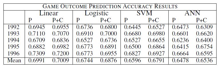
In order to try to answer this question, it is interesting to compare the results obtained in this
project with some other people results. The table below is the results obtained by the NBA oracle
(link for the article in the references). We can observe that the predictions rates obtained are in the
same region and the best result achieved was 0.7009 with the linear regression. Moreover, the
prediction rate of experts are also around 70%.
The small difference obtained in the prediction rate actually corresponds to a considerable
improvement when considering prediction of basketball games. Sports which involves teams, in
general, has many variables associated with the game, for example an injured player. Such variables
were not take into account in this project when using the methods, although an expert can take it
into account. The point is that a prediction rate near experts prediction is actually good.
However, it would be much more interesting if the prediction was higher than experts.
Possible improvements in order to achieve this goal would be to increase the features with some
variables as an injured player, also analyze the player individually and also try to improve the
methods using new configurations or a mixture of methods for example. Obviously, all these
improvements will be hard to be done and, probably, will not represent a very large improvement.Conclusion
This project was very worthy as it has exhibit the practical part of the machine learning. It
has covered the majority part of the steps necessary to use machine learning methods as a important
tool in an application: defining a problem (in our case, to predict NBA games); searching for data;
studying the data; extracting the data from the source and also the features from the data and finally
applying the methods.
Some particular parts as the preparation of data needs a lot of attention as small mistakes can
jeopardize all the data and, consequently, the methods. Other steps as implementing the methods
needs patience to try many configurations. During this project, it became clear that many times the
implementation of the methods is empirical as the math behind methods and the “pattern” behind
the problem can be very complex.
Finally, we can assert that the project has achieved the main purpose that was to consolidate
and reinforce the concepts studied in class and also is a good look into the possibilities of the
machines learning in many applications.References
[1] Matthew Beckler, Hongfei Wang. NBA Oracle
(http://www.mbeckler.org/coursework/2008-2009/10701_report.pdf )
[2] Lori Hoffman Maria Joseph. A Multivariate Statistical Analysis of the NBA
(http://www.units.muohio.edu/sumsri/sumj/2003/NBAstats.pdf )
[3] Osama K. Solieman. Data Mining in Sports:A Research Overview
(http://ai.arizona.edu/mis480/syllabus/6_Osama-DM_in_Sports.pdf )You can also read