Price Discrimination in International Airline Markets - arXiv
←
→
Page content transcription
If your browser does not render page correctly, please read the page content below
Price Discrimination in International Airline Markets∗
                                                    Gaurab Aryal†             Charles Murry‡             Jonathan W. Williams§
arXiv:2102.05751v4 [econ.GN] 20 Apr 2022

                                                                                    April 22, 2022

                                                                                         Abstract

                                                     We develop a model of inter-temporal and intra-temporal price discrimination by
                                                 monopoly airlines to study the ability of different discriminatory pricing mechanisms
                                                 to increase efficiency and the associated distributional implications. To estimate the
                                                 model, we use unique data from international airline markets with flight-level varia-
                                                 tion in prices across time, cabins, and markets and information on passengers’ reasons
                                                 for travel and time of purchase. We find that the current pricing practice yields ap-
                                                 proximately 77% of the first-best welfare. The source of this inefficiency arises pri-
                                                 marily from private information about passenger valuations, not dynamic uncertainty
                                                 about demand. We also find that if airlines could discriminate between business and
                                                 leisure passengers, total welfare would improve at the expense of business passenger
                                                 surplus. Also, replacing the current pricing that involves screening passengers across
                                                 cabin classes with offering a single cabin class has minimal effect on total welfare.

                                             ∗
                                                We are very grateful to the U.S. Department of Commerce for providing the data for our analysis.
                                           We are thankful to research computing facilities at Boston College, UNC and UVA, with special thanks to
                                           Sandeep Sarangi at UNC research computing. Seminar (Arizona, BC, Cornell, Iowa, MIT, Penn State, Rice,
                                           Richmond Fed, Rochester, Texas A&M, Toulouse, UC-Irvine, UNC-Chapel Hill, UWO, WUSTL, Vanderbilt,
                                           Virginia) and conference (SEA 2014, EARIE 2015, IIOC 2016, ASSA 2016, DSE 2019, SITE 2019, QME
                                           2021) participants provided helpful comments. We thank Jan Brueckner, Ben Eden, Gautam Gowrisankaran,
                                           Jacob Gramlich, Qihong Liu, Yao Luo, Brian McManus, Nancy Rose, Nick Rupp, Andrew Sweeting and Peter
                                           R. Hansen for insightful suggestions. All remaining errors are our own.
                                              †
                                                Department of Economics, University of Virginia, aryalg@virginia.edu.
                                              ‡
                                                Department of Economics, Boston College, charles.murry@bc.edu.
                                              §
                                                Department of Economics, University of North Carolina - Chapel Hill, jonwms@unc.edu.

                                                                                             1
1     Introduction
Firms with market power often use discriminatory prices to increase their profits. However,
such price discrimination has ambiguous implications for total welfare. Enhanced price
discrimination may increase welfare by reducing allocative inefficiencies, but it may also
reduce consumer welfare. So an essential aspect of economic- and public-policy towards price
discrimination is to understand how well various discriminatory prices perform in terms of
the total welfare and its distribution, relative to each other and the first-best (e.g., Pigou,
1920; Varian, 1985; Council of Economic Advisors, 2015).
   We evaluate the welfare consequences of price discrimination and quantify sources of in-
efficiencies in a large and economically important setting, international air travel markets.
To that end, we develop and estimate a model of inter-temporal and intra-temporal price
discrimination by a monopoly airline and study how different discriminatory mechanisms
affect welfare and the associated distributional implications. The model incorporates a rich
specification of passenger valuations for two vertically differentiated seat classes on inter-
national flights and a capacity-constrained airline that faces stochastic and time-varying
demand. The airline screens passengers between the two cabins while updating prices and
seat offerings over time. Using the model estimates, we implement various counterfactuals
in the spirit of Bergemann, Brooks, and Morris (2015), where we change the information
the airline has about current and future preferences and measure the welfare under various
discriminatory pricing strategies. Our counterfactual pricing strategies are motivated by cur-
rent airline practices intended to raise profits by reducing allocative inefficiencies, including
attempts to solicit passengers’ reason to travel and use of auctions (Nicas, 2013; Vora, 2014;
Tully, 2015; McCartney, 2016).
   We find that the current pricing practice yields approximately 77% of the first-best wel-
fare; most (87%) of this inefficiency is due to private information about travelers’ valuations,
and the rest (13%) is due to dynamic uncertainty about demand. These results suggest that
airlines’ attempts to collect passenger information for discriminatory pricing could improve
market efficiency. We also find that relative to the current pricing, the ability to screen pas-
sengers based on their reason to travel improves the total welfare at the expense of business
passengers and in favor of the airline and leisure passengers. However, reducing the scope
of second-degree price discrimination by restricting airlines to choose a single price for both
economy and first-class seats each period has a negligible effect on total welfare, suggesting
a strong cross-cabin substitution.
    Our empirical strategy uses a novel dataset of international air travel from the U.S. De-
partment of Commerce’s Survey of International Air Travelers. Compared to data used in the

                                               2
extant literature, the novelty of these data is that we observe both the date of transactions,
ticket prices, and passenger characteristics for dozens of airlines in hundreds of markets. One
such characteristic is the passenger’s reason for travel–business or leisure–which enables us
to study third-degree price discrimination based on passengers’ reasons for travel. Further-
more, there are several highly concentrated nonstop markets in international airline travel,
which allow us to focus on a monopoly pricing model.
   Airlines can segment customers in various ways, enabling them to price discriminate. We
examine ways in which, despite all their advantages, airlines nonetheless are limited in their
ability to price discriminate perfectly. We also document variability and non-monotonicity
in prices before departure, suggesting prices respond to demand uncertainty. In particular,
we document the late arrival of passengers traveling for business, who tend to have inelastic
demand, and the associated changes in prices. Although business travelers’ late arrival puts
upward pressure on fares, fares do not increase monotonically for every flight. This pattern
suggests that the underlying demand for air travel is stochastic and non-stationary.
   We propose a flexible but tractable model of demand and supply to capture these salient
data features. Each period before a flight departs, a random number of nonstop and con-
necting passengers arrive at the marketplace (henceforth, timing of arrivals) and purchase
either a first-class ticket or an economy-class ticket, or decide not to fly at all. Passengers are
short-lived, so those who do not buy a ticket do not remain in or ever return to the market-
place. Our focus is on estimating demand from nonstop travelers, whose willingness-to-pay
depends on the seat class and their reason to travel. We allow the travelers to have different
willingness-to-pay for first-class, such that, for some, the two cabins are close substitutes but
not for others. Furthermore, we allow the mix of business and leisure travelers to vary over
time.
    On the supply side, we model a monopolist airline whose problem is to sell a fixed number
of economy and first-class seats in a finite number of periods to maximize total expected
profit. The airline knows the distribution of passengers’ valuations and the expected number
of nonstop and connecting arrivals, and each period it chooses prices and seats to release
before observing the demand.1 We assume that the future arrival process is not affected
by the airline’s choices, and thus the number of unsold seats is the only endogenous state
variable. Thus, every period before the flight, the airline balances the expected profit from
selling a seat today against the forgone future expected profit. This inter-temporal trade-
off results in a time-specific endogenous opportunity cost for each seat that varies with the
expected future demand and number of unsold seats.
   1
     We model the airline committing to a seat release policy to mimic the “fare bucket” strategy used by
airlines in practice. See, for example, Alderighi, Nicolini, and Piga (2015) for more on these buckets.

                                                   3
Besides this temporal consideration, each period, the airline screens passengers between
two cabins. Thus, our model captures the inter -temporal and intra-temporal aspects of price
discrimination by airlines. Moreover, these temporal and intra-temporal considerations are
interrelated. For instance, if the airline increases the price for economy seats today, it will
trade off fewer economy sales today, higher first-class sales today, with higher economy and
lower first-class sales in the future. As demand varies over time, these trade-offs vary too.
The estimation of our model presents numerous challenges. The demand and supply
specifications result in a non-stationary dynamic programming problem that involves solving
a mixed-integer nonlinear program for each state. We solve this problem to determine optimal
prices and seat-release policies for every possible combination of unsold seats and days until
departure. Moreover, our data include numerous flights across hundreds of routes, so not
only do we allow for heterogeneity in preferences across passengers within a flight, we also
allow different flights to have different distributions of passenger preferences.
To estimate the model and recover the distribution of preferences across flights, we
use a simulated method of moments approach based on the importance sampling proce-
dure of Ackerberg (2009). Similar approache to estimate a random coefficient specifica-
tion has been used by Fox, Kim, and Yang (2016), Nevo, Turner, and Williams (2016), and
Blundell, Gowrisankaran, and Langer (2020). Like them, we match empirical moments and
model-implied moments describing within- and across-flight variation in fares and purchases.
Our estimates suggest substantial heterogeneity across passengers within and across
flights. The estimated marginal distributions of the willingness-to-pay for one-way travel
for business and leisure travelers are consistent with the observed distribution of fares, with
average willingness-to-pay for an economy seat by leisure and business travelers being $392
and $537, respectively. Furthermore, on average, passengers value a first-class seat 58%
more than an economy seat, implying meaningful cross-cabin substitution. The arrivals of
nonstop and connecting passengers decline in the run-up to the flight. However, among the
nonstop arrivals, the share of business travelers increases from zero to almost 30% for the
average flight. We calculate the time-specific opportunity cost of selling a seat using the
model estimates, which provides novel insight into airlines’ dynamic incentives.
Using the estimates and the model, we characterize the level of efficiency and the associ-
ated distribution of surplus for alternative pricing mechanisms that provide new insights into
the welfare consequences of price discrimination. Regarding efficiency, airlines’ current pric-
ing practices are similar to a scenario where we prohibit them from charging multiple prices
across cabins. We also find that the current pricing achieves 77% of the first-best welfare, and
most (87%) of this inefficiency is due to private information about the passengers’ valuations.
When determining when these efficiency losses occur, we find that most inefficiencies occur
4in the earlier periods. Airlines sell too many seats from a total efficiency standpoint early in
the sales process due to uncertainties about passenger willingness to pay and future arrivals,
thus excluding potentially high-surplus late-arriving passengers. We find that third-degree
price discrimination based on the reason to travel–business or leisure–improves total surplus
but lowers consumer surplus.
Regarding the surplus distribution between airlines and passengers, we find that price
discrimination skews the distribution of surplus in favor of the airlines. In particular, the gap
between producer and consumer surplus increases by approximately 25% when airlines price
differently across cabins, compared to setting only one price per period for both cabins. If
an airline were to price discriminate even more based on reasons to travel, it would increase
the airline’s share of surpluses. We illustrate the effect of airlines knowing the reason to
travel on welfare by determining surplus division when the airline does not know the reason
to travel and uses a Vickery-Clarke-Grove (VCG) auction, period-by-period. We find that
using VCG auctions more than doubles the consumer surplus under current pricing practices
and is as efficient as eliminating all static informational frictions.
Contribution and Related Literature. Our paper relates to vast research on the eco-
nomics of price discrimination and research in the empirical industrial organization on esti-
mating the efficiency and division of welfare under asymmetric information. Most of these pa-
pers, however, focus on either cross-sectional price discrimination (e.g., Ivaldi and Martimort,
1994; Leslie, 2004; Busse and Rysman, 2005; Crawford and Shum, 2006; Mortimer, 2007;
McManus, 2007; Aryal and Gabrielli, 2019) or inter-temporal price discrimination dynamics
(e.g., Nevo and Wolfram, 2002; Nair, 2007; Escobari, 2012; Jian, 2012; Hendel and Nevo,
2013; Lazarev, 2013; Cho et al., 2018), but not both.
We also contribute to the literature that focuses on dynamic pricing (e.g., Graddy and Hall,
2011; Sweeting, 2010; Cho et al., 2018; Waisman, 2021). However, none studies intra-
temporal price discrimination, inter-temporal price discrimination, and dynamic pricing to-
gether, even though many industries involve all three. Relatedly, Coey, Larsen, and Platt
(2020) document inter-temporal and intra-temporal price dispersion in an environment with
consumer search and deadlines but without price discrimination. We contribute to this re-
search by developing an empirical framework where both static discriminative pricing and
dynamic pricing incentives are present and obtain results that characterize the welfare im-
plications.2 Our welfare analysis has some similarities with Dubé and Misra (Forthcoming)
2
There is a long and active theoretical literature on static and inter-temporal price discrimination; see
Stokey (1979); Gale and Holmes (1993); Dana (1999); Courty and Li (2000); Armstrong (2006) and refer-
ences therein. Airline pricing has also been studied extensively from the perspective of revenue management ;
see van Ryzin and Talluri (2005).
5and Williams (2022), who find that price discrimination improves welfare.
Additionally, we complement recent research related specifically to airline pricing, partic-
ularly Lazarev (2013), Li, Granados, and Netessine (2014), and Williams (2022).3 Lazarev
(2013) considers a model of inter-temporal price discrimination with one service cabin and
finds large potential gains from allowing reallocation among passengers arriving at different
times before the flight. Like us Williams (2022) further allows for dynamic adjustment of
prices in response to stochastic demand and finds that dynamic pricing (relative to a single
price) increases total welfare at the expense of relatively inelastic customers who arrive late.
Our paper, however, differs from the existing literature on price discrimination in several
ways. First, we model both inter-temporal and intra-temporal price discrimination, closely
capturing a multiproduct airline’s decisions to screen passengers between cabin classes. Our
results suggest that these two aspects jointly affect welfare. Second, like Lazarev (2013)
we model connecting passengers, who play an important role in dynamic adjustments to
remaining seats. Third, we model the airlines’ ability to choose the number of seats avail-
able to passengers at any given time before the flight, which mimics the complicated selling
algorithms that airlines use in practice. Lastly, we observe passengers’ reasons for traveling,
so we can measure business and leisure passenger welfare.
Most papers use a random utility discrete choice framework to model the demand for
air travel (e.g., Berry, Carnall, and Spiller, 2006). Instead, we use a pure characteristics
approach, following the theoretical literature on price discrimination (e.g., Mussa and Rosen,
1978). See also Berry and Pakes (2007) and Barseghyan, Molinari, and Thirkettle (2021)
for empirical examples. A pure characteristic approach is natural when modeling purely
vertical product differentiation, in our case, economy and premium-class cabins. We estimate
a flexible random coefficients demand model that captures within-flight and across-flight
heterogeneity in consumer preferences. This approach is important, as we have data for
many types of flights. The richness in our specification allows us to capture variation in
demand parameters due to permanent and unobserved differences across markets. However,
the flexibility of our random-effects approach comes at the cost of not modeling flight-specific
variables that predict demand.
2 Data
The Department of Commerce’s Survey of International Air Travelers (SIAT) gathers infor-
mation on international air passengers traveling to and from the U.S. Passengers are asked
3
Also see Borenstein and Rose (1994), Puller, Sengupta, and Wiggins (2012); Chandra and Lederman
(2018), who use a regression approach to study effects of oligopoly on dispersion in airfares.
6detailed questions about their flight itinerary, either during the flight or at the gate area
before the flight. The SIAT targets both U.S. residents traveling abroad and non-residents
visiting the U.S. Passengers in our sample are from randomly chosen flights from among
more than 70 participating U.S. and international airlines, including some charter carriers.
The survey contains ticket information, which includes the cabin class (first, business, or
economy), date of purchase, total fare, and the trip’s purpose (business or leisure). We
combine fares reported as business class and first-class into a single cabin class that we label
“first-class.” This richness distinguishes the SIAT data from other data like the Origin and
Destination Survey (DB1B) conducted by the Department of Transportation. In particular,
the additional details about passengers (e.g., time of purchase, individual ticket fares, and
reason for travel) make the SIAT dataset ideal for studying price discrimination.
We create a dataset from the survey where a unit of observation is a single ticket purchased
by a passenger flying a nonstop (or direct) route. We then use fares and purchase (calendar)
dates associated with these tickets to estimate price paths for each flight in our data, where
a flight is a single instance of a plane serving a particular route. For example, in our sample,
we observe some nonstop passengers flying United Airlines from SEA to TPE on August 12,
2010, departing at 5:10 pm, then we say that this is one flight. From the data on fares and
dates for this flight, we use kernel regression to estimate price paths for economy seats and
first-class seats leading up to August 12, 2010. In this section, we detail how we selected the
sample and display descriptive statistics that motivate our model and analysis.
2.1 Sample Selection
Our sample from the DOC includes 413,309 passenger responses for 2009-2011. We clean the
data to remove contaminated and missing observations and to construct a sample of flights
that will inform our model of airline pricing, which we specify in the following section.
We detail our sample selection procedure in Appendix A.1, but, for example, we exclude
responses that do not report a fare, are part of a group travel package, or are non-revenue
tickets. We supplement our data with schedule data from the Official Aviation Guide of the
Airways (OAG) company, which reports cabin-specific capacities, by flight number. Using
the flight date and flight number in SIAT we can merge the two data sets. We include flights
for which we observe at least ten nonstop tickets after applying the sample selection criteria.
Monopoly Markets. As mentioned earlier, we focus on monopoly markets. In inter-
national air travel, nonstop markets tend to be concentrated for all but the few busiest
airport-pairs. We classify a market as a monopoly market if it satisfies one of following
two criteria: (i) one airline flies at least 95% of the total capacity on the route (where the
7capacity is measured using the OAG data); or (ii) a US carrier and foreign carrier operate on
the market with antitrust immunity from the U.S. Department of Justice. These immunities
do not have any additional regulatory oversight on airfares.
These antitrust exemptions come from market access treaties signed between the U.S.
and the foreign country that specify a local foreign carrier (usually an alliance partner of the
U.S. airline) that will share the route. For example, on July 20, 2010, antitrust exemption
was granted to OneWorld alliance, which includes American Airlines, British Airways, Iberia,
Finnair and Royal Jordanian, for 10 years subject to a slot remedy.4
In a few cases, we define markets at the city-pair level because we are concerned that
within-city airports are substitutable. The airports that we aggregate up to a city-pairs
market definition include airports in the New York, London, and Tokyo metropolitan. Thus,
we treat a flight from New York JFK to London Heathrow to be in the same market as a
flight from Newark EWR to London Gatwick.
Table 1: Top 20 Markets, Ordered by Sample Representation
Unique Distance Unique Distance
Market Flights Obs. (miles) Market Flights Obs. (miles)
Los Angeles (LAX)-Shanghai (PVG) 53 1,646 6,485 New York (JFK)-Vargas (CCS) 20 476 2,109
San Francisco (SFO)-Auckland (AKL) 28 1,623 6,516 Boston (BOS)-Keflavik (KEF) 13 427 2,413
New York (JFK)-Helsinki (HEL) 35 1,191 4,117 New York (JFK)-Santiago (SCL) 16 423 5,096
New York (JFK)-Johannesburg (JNB) 26 1,035 7,967 New York (JFK)-Nice (NCE) 9 329 3,991
New York (JFK)-Warsaw (WAW) 34 787 4,267 New York (JFK)- Dubai (DXB) 9 325 6,849
New York (JFK)-Vienna (VIE) 29 729 4,239 Pheonix (PHX)-Puerto Vallarta (PVR) 6 289 971
Phoenix (PHX)-Cabo (SJD) 18 703 721 Orlando (MCO)-Frankfurt (FRA) 8 284 4,734
New York (JFK)-Casablanca (CMN) 21 625 3,609 San Francisco (SFO)-Paris (CDG) 10 251 5,583
Seattle (SEA)-Taipei (TPE) 21 328 6,074 San Francisco (SFO)- Tokyo (HND) 4 251 5,161
New York (JFK)-Buenos Aires (EZE) 24 547 5,281 Orlando (SFB)-Birmingham (BHX) 10 245 4,249
Note: The table displays the Top 20 markets, their representation in our sample, their distance (air miles) from U.S. Data from
the Survey of International Air Travelers and sample described in the text.
Description of Markets and Carriers. After our initial selection and restriction on
nonstop monopoly markets, we have 14,930 observations representing 224 markets and 64
carriers. We list the top 20 markets based on sample representation in Table 1, along with
the number of unique flights and the total observations. The most common U.S. airports in
our final sample are New York JFK (JFK), San Francisco (SFO), and Phoenix (PHX), and
the three most common routes are Los Angeles to Shanghai, China (PVG), San Francisco
to Auckland, New Zealand (AKL), and New York to Helsinki, Finland (HEL). The median
flight has a distance of 4,229 miles, and the inter-quartile range of 2, 287 to 5, 583 miles. In
Table 2 we display the top ten carriers from our final sample, which represent approximately
60% of our final observations.
4
To determine such markets, we use information from DOT and carriers’ 10K reports filed with the SEC.
8Table 2: Top Ten Carriers, Ordered by Sample Representation
Carrier Unique Flights Obs.
US Airways 77 3,179
Continental 98 2,036
American Airlines 88 1,926
Air New Zealand 30 1,666
China Eastern 53 1,646
Finnair 35 1,191
Lufthansa 40 1,079
Delta 35 1,062
South African 26 1,035
Austrian 35 881
Note: The table displays the top ten carriers, ordered by their frequency in the final sample. Data from the Survey of
International Air Travelers and sample described in the text.
2.2 Passenger Arrivals and Ticket Sale Process
Passengers differ in terms of time of purchases and reasons for travel, and prices vary over
time and across cabins. In this subsection we present key features in our data pertaining to
passengers and prices.
Timing of Purchase. Airlines typically start selling tickets a year before the flight date.
Although passengers can buy their tickets throughout the year, in our sample most passengers
buy in the last 120 days. To keep the model and estimation tractable, we classify the purchase
day into a fixed number of bins. At least two factors motivate our choice of bin sizes. First,
it appears that airlines typically adjust fares frequently in the last few weeks before the
flight date, but less often farther away from the flight date. Second, there is usually a
spike in passengers buying tickets at focal points, like 30 days, 60 days etc. Although, in
our model, we focus on pricing and seat release decisions in monopoly markets for nonstop
travel, flights also have connecting passengers. For example, in the LAX-PVG market, there
can be nonstop passengers whose trips originate in LAX and terminate in PVG, but there
may also be those flying from SFO (or other originating airports) to PVG via LAX. In
Table 3 we present eight fixed bins for nonstop and connecting passengers, and the number
of observations in each bin. We use narrower bins when closer to the flight date to reflect
the dynamic pricing strategies used by airlines. Each of these eight bins corresponds to one
period, giving us a total of eight periods.
Passenger Characteristics. We classify each passenger as either a business traveler or
a leisure traveler based on the reason to travel. Business includes business, conference, and
9Table 3: Distribution of Advance Purchase
Days Until Flight Nonstop Obs. Connecting Obs.
0 − 3 days 597 437
4 − 7 days 753 528
8 − 14 days 1,038 839
15 − 29 days 1,555 1,126
30 − 44 days 2,485 1,855
45 − 60 days 2,561 1,936
61 − 100 days 2,438 1,800
101+ days 3,400 2,332
Note: The table displays the distribution of advance purchases. First column is the number of days before flight, and the second
and third columns show how many nonstop and connecting passengers bought their tickets in those days, respectively.
government or military, while leisure includes visiting family, vacation, religious purposes,
study or teaching, health, and other; see Table A.1.1 for more.5 We classify service cabins
into economy class and first-class, where we combine business and first class as the latter.6
In Table 4 we display some key statistics for relevant ticket characteristics in our nonstop
sample. As is common in the literature, to make one-way and round-trip fares comparable
we divide round-trip fares by two. Approximately 4.5% passengers report to have bought a
one-way ticket; see Table A.1.1. The standard deviations in fares, which quantify both the
across-market and within-flight variation in fares, are large, with the coefficient of variation
0.85 for economy and 1.06 for first-class.
In the second panel of Table 4, we display the same statistics by the number of days in
advance of a flight’s departure that the ticket was purchased (aggregated to eight “periods”).
We see that while the average fare increases for tickets purchased closer to the departure
date, so does the standard deviation.
Similarly, at the bottom panel of Table 4, we report price statistics by the passenger’s
trip purpose. About 14% of the passengers in our sample flew for business purposes, and
these passengers paid an average price of $684 for one direction of their itinerary. Leisure
passengers paid an average of $446. This price difference arises for at least three reasons:
business travelers tend to buy their tickets much closer to the flight date, they prefer first-
class seats, and they fly different types of markets.
In Figure 1(a) we plot the average price for economy fares as a function when the ticket
was purchased. Both business and leisure travelers pay more if they buy the ticket closer
to the flight date, but the increase is more substantial for the business travelers. The solid
line in Figure 1(a) reflects the average price across both reasons for travel. At earlier dates,
5
We also observe the channel through which the tickets were purchased: travel agents (36.47%), personal
computer (39.76%), airlines (13.36%), company travel department (3.99%), and others (6.42%).
6
For 90% of the flights, passengers are seated in only one of these two (business- and first-class cabins),
but not both.
10Table 4: Summary Statistics from SIAT, Ticket Characteristics of Nonstop Passengers
Proportion Fare
Ticket Class of Sample Mean S.D.
Economy 92.50 447 382
First 7.50 897 956
Advance Purchase
0-3 Days 4.03 617 636
4-7 Days 5.08 632 679
8-14 Days 7.00 571 599
15-29 Days 10.49 553 567
30-44 Days 16.76 478 429
45-60 Days 17.27 467 432
61-100 Days 16.44 414 315
101+ Days 22.93 419 387
Travel Purpose
Leisure 85.57 446 400
Business 14.43 684 716
Note: Data from the Survey of International Air Travelers. Sample described in
the text.
Figure 1: Business versus Leisure Passengers before the Flight Date
600 0.35
0.3
550
0.25
0.2
500
0.15
0.1
450
0.05
400 0
17 16 15 14 13 12 11 10 9 8 7 6 5 4 3 2 1 0 17 16 15 14 13 12 11 10 9 8 7 6 5 4 3 2 1 0
(a) Average Economy Fares Prior to Flight (b) Business and Leisure Travelers
Note: (a) Average price paths across all flights for tickets in economy class by week of purchase prior to the flight date, by
self-reported business and leisure travelers. Individual transaction prices are smoothed using nearest neighbor with a Gaussian
kernel with optimal bandwidth of 0.5198. (b) Proportion of business passengers across all flights, by advance purchase weeks.
11the total average price is closer to the average price paid by leisure travelers, while it gets
closer to the average price paid by the business travelers as the date of the flight nears. In
Figure 1(b), we display the proportion of business to leisure travelers across all flights, by the
advance purchase categories. In the last two months before flight, the share of passengers
traveling for leisure is approximately 90%, which decreases to 65% a week before flight.
Taken together, business travelers purchase closer to the flight date than leisure travelers,
and markets with a greater proportion of business travelers have a steeper price gradient.
Figure 2: Histogram of Percent of Nonstop Business Passengers by Flight
Note: Histogram of business-travel index (BTI). The business-traveler index is the flight-specific ratio of self-reported business
travelers to leisure travelers. The mean is 0.154 and the standard deviation is 0.210.
Observing the purpose of travel plays an important role in our empirical analysis, reflect-
ing substantial differences in the behavior and preferences of business and leisure passengers.
This passenger heterogeneity across markets drives variation in pricing, and this covariation
permits us to estimate a model with richer consumer heterogeneity than the existing liter-
ature like Berry, Carnall, and Spiller (2006) and Ciliberto and Williams (2014). Further, a
clean taxonomy of passenger types allows a straightforward exploration of the role of asym-
metric information in determining inefficiencies and the distribution of surplus that arises
from discriminatory pricing of different forms.7
To further explore the influence that this source of observable passenger heterogeneity
7
Passengers can also use reward points to buy their ticket, but we do not consider those tickets here.
However, reward points are not common in our data. Only 3.5% of tickets are bought using reward points,
and 5.46% of passengers report that the main reason why they choose their airline is frequent-flyer miles. In
our final (estimation) sample, 1.7% passengers get upgraded, i.e., they buy economy but fly first-class. Our
working hypothesis is that those upgrades materialized only on the day of travel.
12has on fares, we present statistics on across-market variation in the dynamics of fares. Specif-
ically, we first calculate the proportion of business travelers in each market, i.e., across all
flights with the same origin and destination. Like Borenstein (2010), we call this market-
specific ratio the business-traveler index (BTI). In Figure 2, we present the histogram of the
BTI across markets in our data. If airlines know of this across-market heterogeneity and
use it as a basis to discriminate both intra-temporally (across cabins) and inter-temporally
(across time before a flight departs), different within-flight temporal patterns in fares should
arise for different values of the BTI.
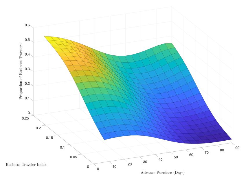
Figure 3: Proportion of Business Travelers by Ticket Class
(a) Economy Class (b) First-Class
Note: The figure presents kernel regression of reason to travel on BTI and the purchase date. Panels (a) and (b) show the
regression for economy and the first-class seats, respectively. The regression uses a Gaussian kernel with optimal “rule-of-thumb”
bandwidth.
In Figure 3 we present the results of a bivariate kernel regression where we regress an
indicator for whether a passenger is traveling for business on the BTI in that market and
number of days the ticket was purchased in advance of the flight’s departure. Figures 3(a)
and 3(b) present the results for economy and first-class passengers, respectively. There are
two important observations. First, across all values of the BTI, business passengers arrive
later than leisure passengers. Second, business passengers disproportionately choose first-
class seats. To capture this feature, in Section 3, we model the difference between business
and leisure passengers in terms of the timing of purchases and the preference for quality
by allowing the passenger mix to change as the flight date approaches, resulting in a non-
stationary demand process.
The influence of business passengers is evident on prices. Like Figure 3, Figure 4(a) and
Figure 4(b) present the results of a kernel regression with fare paid as the dependent variable
for economy and first-class cabins, respectively. In both, we present cross-sections of these
13Figure 4: Across-Market Variation in Fares
580 1300
560
1200
540
520 1100
500
1000
480
900
460
440 800
420
700
400
380 600
70 60 50 40 30 20 10 0 70 60 50 40 30 20 10 0
(a) Economy (b) First-Class
Note: The figure presents results from a kernel regression of fares paid on BTI and the purchase date. Panels (a) and (b) show
the results from the regression evaluated at different values of BTI, for economy and the first-class seats, respectively. The
regression uses a Gaussian kernel with optimal “rule-of-thumb” bandwidth.
estimated surfaces for the 25th , 50th , and 75th percentile values of the BTI. For both cabins,
greater values of the BTI are associated with substantially higher fares.
While there are clear patterns in how the dynamics of average fares vary with the BTI,
there is also substantial heterogeneity across flights in how fares change as the flight date
approaches. Furthermore, the fares are non-monotonic in arrival time. To see the non-
monotonicity in temporal patterns for individual flights that Figure 3 masks, Figure 5
presents the time-paths of economy fares for all flights in our data. Specifically, for each
flight, we estimate a smooth relationship between economy fares and time before departure
using a kernel regression, and then normalize the path relative to the initial fare we observe
for that flight for that flight. Each line is a single flight from our data, and begins when we
first observe a fare for that flight, and ends at 1, the day of the flight.
For most flights we observe little movement in fares until approximately 100 days before
departure. Yet, for a small proportion of flights, there are substantial decreases and increases
in fares as much as 5 months before departure. Further, by the date of departure, the
interquartile range of the ratio of current fare to initial fare is 0.75 to 1.85. Thus, 25% of
flights experience a decrease of more than 25%, while 25% of flights experience an increase of
greater than 85%. The variation in the temporal patterns in fares across flights is attributable
to both the across-market heterogeneity in the mix of passengers, and how airlines respond
to demand uncertainty.
14Figure 5: Flight-Level Dispersion in Fares
3
2.5
Normalized Fare
2
1.5
1
0.5
0
150 100 50 0
Days until Flight
Note: The figure presents the estimated fare paths from every flight we use in our estimation. Each line represents a flight.
We normalize the fares to unity by dividing fares by the first fare we observe for the flight. The horizontal axis represents the
number of days until the flight, where zero is the flight date.
2.3 Aircraft Characteristics
Airlines’ fares, and how they respond to realized demand, depend on the number of unsold
seats. In Figure 6(a), we display the joint density of initial capacity of first and economy
class in our sample. The smaller of the two peaks corresponds to approximately 160 economy
seats and 18 first-class seats, and the higher peak corresponds to approximately 265 economy
seats and 47 first-class seats.
Figure 6: Initial Capacity and Load Factor
(a) Density of Initial Capacities (b) Histogram of Load Factor
Note: In part (a), this figure presents the Parzen-Rosenblatt Kernel density estimate of the joint-density of initial capacities
available for nonstop travel. In part (b), this figure presents the histogram of the passenger load factor across our sample.
The five most common aircraft types in our sample are the Boeing 777 (23%), 767 (13%),
757 (13%), 737 (12%), and the Airbus A340 (8%). The 777, 747, and A340 are wide-body
15jets used typically on long-haul flights, and they roughly correspond to the higher of the two
peaks in Figure 6(a). The 737 has a typical configuration of around 160 seats, which roughly
corresponds to the smaller of the two peaks in Figure 6(a). We refer to these two peaks as
small and large modal capacity. Furthermore, the exact capacity configurations change from
flight to flight.
If we take the proportion of economy seats to the total seats for each flight and average
across all flights in our sample, we find that 88% of all seats are economy class. We merge the
SIAT data with the Department of Transportation’s T-100 segment data to get a measure
of the load factor, which is defined as the ratio of the total number of seats sold by the day
of the flight to the total number of seats available in the aircraft, for our SIAT flights. From
the T100, we know the average load factor across a month for a particular route flown by a
particular type of equipment. In Figure 6(b), we display the histogram of load factor across
flights in our sample. The median load factor is 82%, but substantial heterogeneity exists
across flights.
Overall, our descriptive analysis reveals several salient features that we capture in our
model. We find that a business-leisure taxonomy of passenger types is helpful to capture
differences in the timing of purchase, willingness-to-pay for an economy seat and a vertically
differentiated first-class seat. Further, we find evidence consistent with airlines responding to
substantial heterogeneity in the business or leisure mix of passengers across markets, creating
variation in both the level and temporal patterns of fares across markets. Finally, across
flights, we observe considerable heterogeneity in fare paths as the flight date approaches.
Together, these features motivate our model of non-stationary and stochastic demand and
dynamic pricing by airlines that we present in Section 3, as well as the estimation approach
in Section 4.
3 Model
In this section, we present a model of dynamic pricing by a profit-maximizing multi-product
monopoly airline that sells a fixed number of economy seats (0 ≤ K e < ∞) and first-class
seats (0 ≤ K f < ∞) on a flight. We assume that nonstop passengers with heterogeneous
and privately known preferences (i.e., their willingness-to-pay for an economy and first-class
seat) arrive before the date of departure (T ). Additionally, the plane’s capacity is occupied
by passengers that use the flight segment as part of a multi-segment trip. Every period the
airline has to choose the ticket prices and the maximum number of seats to release at those
prices before it realizes the demand (for that period).
Our data indicate essential sources of heterogeneity in preferences that differ by reason-
16for-travel and purchase timing. Further, variability and non-monotonicity in observed fares
suggest a role for uncertain demand. Our demand-side model seeks to flexibly capture this
multi-dimensional heterogeneity and uncertainty that serves as an input into the airline’s
dynamic-pricing problem. Furthermore, our supply-side model seeks to capture the inter-
temporal and intra-temporal trade-offs faced by an airline in choosing its optimal policy.
3.1 Demand
Let Nt denote the number of nonstop individuals that arrive in period t ∈ {1, . . . , T } to
consider buying a nonstop ticket, where T < ∞ is the flight date. We model Nt as a Poisson
random variable with parameter λnt ∈ R+ , i.e., E(Nt ) = λnt . Additionally, let Ct denote the
number of connecting passengers that utilize the airplane in period t ∈ {1, . . . , T }. We model
Ct also as a Poisson random variable with parameter λct ∈ R+ , i.e., E(Ct ) = λct . The airline
knows (λnt , λct ) for t ∈ {1, . . . , T }, but must make pricing and seat-release decisions before the
uncertainty over the realized number of arrivals is resolved each period. The nonstop arrivals
are one of two types, for-business or for-leisure. The probability that a given individual is
for-business varies across time before departure and denoted by θt ∈ [0, 1].
To model individual preferences of nonstop passengers, we use a pure characteristics ap-
proach (e.g., Mussa and Rosen, 1978; Berry and Pakes, 2007; Barseghyan, Molinari, and Thirkettle,
2021). Passengers have different willingness-to-pay for flying, but everyone prefers a first-
class seat to an economy seat. Let v ⊂ R+ denote the value a passenger assigns to flying in
the economy cabin, and let the indirect utility of this individual from flying economy and
first-class at a price p, respectively, be
ue (v, p, ξ) = v − p; uf (v, p, ξ) = v × ξ − p, ξ ∈ [1, ∞).
The (utility) premium associated with flying in a first-class seat, ξ captures the vertical
quality differences between the two cabins. Passengers are heterogeneous in terms of their v
and ξ, and v and ξ are independent and privately known to the individual. Thus, we assume
that utility from the outside option, which includes either not flying or flying through other
routes, is normalized to zero.
We assume that the preferences across passengers are realizations from type-specific dis-
tributions. Specifically, the v of for-business and for-leisure arrivals are drawn from Fvb (·) and
Fvl (·), respectively, and ξ is drawn from Fξ (·). Together with the arrival process, the type-
specific distribution of valuations creates a stochastic and non-stationary demand process
that we assume is known to the airline.
At given prices and a given number of seats available at those prices, Figure 7 summarizes
17Figure 7: Realization of Demand of Nonstop Arrivals
Airline Chooses: (pet , qet ), (pft , q ft )
Individuals Arrive : Nt ∼ P(λnt )
Business: θt Leisure: 1 − θt
Business Arrivals: Ntb Leisure Arrivals: Ntl
(vi , ξi ) ∼ Fvb × Fξ , i = 1, . . . , Ntb (vi , ξi ) ∼ Fvl × Fξ , i = 1, . . . , Ntl
Buy: qte , qtf ; Not Buy: qto
q et ≥ qte q et < qte q et ≥ qte q et < qte
qft ≥ qtf qft ≥ qtf qft < qtf qft < qtf
(Case A) (Case B) (Case C) (Case D)
Not binding Economy-class First-class Both-classes
binding binding binding
Note: A schematic representation of the timing of demand for nonstop arrivals.
18a realization of the demand process for period t for nonstop passengers. Specifically, the
realization of demand and timing of information known by the airline leading up to a flight’s
departure is as follows:
(i) Airline chooses a price and seat-release policy for economy cabin, (pet , q et ), and the
first-class cabin, (pft , qft ), that determine the prices at which a maximum number
of seats in the two cabins may be sold.
(ii) Nt many nonstop individuals arrive, the number being drawn from a Poisson
distribution with parameter λnt . Each arrival realizes their reason to fly from
a Bernoulli distribution with parameter θt (i.e., for-business equals one). Each
arrival observes their own (v, ξ), drawn from the respective distributions, Fvb (·),
Fvl (·), and Fξ (·).
(iii) Ct many connecting individuals arrive, the number is drawn from a Poisson dis-
tribution with parameter λct . A connecting arrival is assigned as a potential
economy-cabin passenger with a fixed probability r and a potential first-class
passenger with the complementary probability.
(iv) The nonstop and connecting arrivals are allocated a seat alternatingly, but con-
ditional on that, the seats are randomly allocated among either nonstop or con-
necting arrivals. Thus, connecting passengers affect only the seats available for
nonstop passengers.
(v) If neither seat-release policy is binding (realized demand does not exceed the
number of seats released in either cabin), arrivals select their most preferred cabin:
first-class if v × ξ − pft ≥ max{0, v − pet }, economy if v − pet ≥ max{0, v × ξ − pft },
and no purchase if 0 ≥ max{v × ξ − pft , v − pet }. Those arrivals choosing the
no-purchase option leave the market and never return. If the seat-release policy
is binding in either one or both cabins, we assume that arrivals make sequential
decisions in a randomized order until either none remaining wishes to travel in
the cabin with capacity remaining, or all available seats are allocated.
(vi) If there are more connecting arrivals than nonstop, then the connecting arrivals
are allocated until none are left, or a capacity binds.
(vii) Steps (i)-(iv) repeat until the departure date, t = T , or all seats are allocated.
In any given period (t), there are four possible outcomes given a demand realization:
neither seat-release policy is binding, either one of the two seat-release policies is binding, or
19both are binding. If the seat-release policy is not binding for either of the two cabins, then
the expected demand for the respective cabins in period t when the airline chooses policy
χt := (pet , qet , pft , q ft ) is
∞
X
Et (q e ; χt ) := n × Pr(Nt = n) Pr(v − pet ≥ max{0, v × ξ − pft }) = λt × Pte (χt );
| {z }
n=0
:=Pte (χt )
∞
X
f
Et (q ; χt ) := f
n × Pr(Nt = n) Pr(v × ξ − pt ≥ max{0, v − pt }) = λt × Ptf (χt ).
e
| {z }
n=0 f
:=Pt (χt )
If one or both of the seat-release policies are binding, the rationing process creates the
possibility for inefficiencies to arise both in terms of exclusion of passengers with a greater
willingness-to-pay than those allocated a seat, as well as misallocations of passengers across
cabins.
In Figure 8, we present a simple example to illustrate inefficiency arising from asymmetric
information in this environment under random allocation. Assume the airline has one first-
class and two economy seats remaining and chooses to release one seat in each cabin at
pf = 2000 and pe = 500. Suppose three nonstop passengers arrive with values v1 = 2500,
v2 = 1600, and v3 = 5000, with ξ1 = ξ2 = 2 and ξ3 = 1. Arrivals n1 and n2 are willing to
pay twice as much for a first-class seat as an economy seat, whereas arrival n3 values the
two cabins equally. Furthermore, suppose two connecting passengers arrive, and out of these
two, suppose the first connecting arrival c1 is to be allocated an economy seat, and c2 is to
be allocated a first-class seat, if available. Suppose that under the random allocation rule,
nonstop arrivals get to choose before connecting, and among nonstop arrivals, n2 gets to
choose first, and n3 is the last, and among connecting arrivals, suppose c1 is allocated first.
As shown in Figure 8, the final allocation is inefficient because a) arrival n2 gets first-class
even though n1 values it more; and b) both nonstop arrivals n1 and n3 do not get any seat.
This difference in arrival timing creates the possibility for multiple welfare-enhancing trades.
Given the limited opportunity for coordination among arrivals to make such trades and the
legal or administrative barriers, we believe random rationing is reasonable to allocate seats
within a period.8
8
Passengers considering flying are not always in the marketplace, looking for the best deal on tickets.
They arrive at different times for exogenous reasons. Random rationing captures this realistic feature of the
data. The seat release policies, presence of connecting passengers, and random assignments imply that there
may be instances when a potential passenger with a high willingness-to-pay shows up to the market and
cannot be served because a low willingness-to-pay passenger who arrived earlier was allocated the seat. If
instead, we use optimal rationing, where seats are assigned in the order of willingness-to-pay, it would lead
to higher baseline efficiency
20Figure 8: Illustration of Random Rationing Rule.
prices pf = 2000; qf = 1
Capacity: K f = 1, K e = 2
seats pe = 500, qe = 1
demand realization
v1 = 1800 v2 = 1600, v3 = 1900
ξ1 = 2, ξ2 = 2, ξ3 = 1
preference ordering
nonstop passenger-id preference passenger-order allocation
yes n1 f ≻e≻o n2 f
yes n2 f ≻e≻o random c1 e
yes n3 e≻o≻f allocation n1 o
no c1 − n3 o
no c2 − c2 o
Note: Example to demonstrate how random-rationing rule can generate inefficiency in the model.
3.2 Supply
The airline has T periods before the departure to sell K e and K f economy and first-class
seats, respectively. Each period, the airline chooses prices {pet , pft } and commits to selling no
more than {qet , q ft } ≤ ωt seats at those prices, where ωt := (Kte , Ktf ) is the number of unsold
seats in each cabin. We model that airlines must commit to a seat-release policy to mimic
the “fare bucket” strategy that airlines use in practice (e.g., Alderighi, Nicolini, and Piga,
2015), which helps the airline insure against a favorable demand shock where too many seats
are sold today at the expense of future passengers with higher willingness-to-pay. One of
this market’s defining characteristics is that the airline must commit to policies every period
before realizing the demand. The airline does not observe a passenger’s reason to fly or
valuations (v, ξ); however, the airline knows the underlying stochastic process that governs
demand and uses the information to price discriminate, both within and across periods.9
Let ce and cf denote the constant cost of servicing a passenger in the respective cabins.
These marginal costs, or so-called “peanut costs,” capture variable costs like food and bever-
age service that do not vary with the timing of the purchase but may vary with the different
levels of service in the two cabins. Let Ψ := ({Fvb , Fvl , Fξ , cf , ce }, {λt, θt , γt }Tt=1 ) denote the
9
See Barnhart, Belobaba, and Odoni (2003) for an overview of forecasting airline demand.
21vector of demand and cost primitives.
The airline maximizes the sum of discounted expected
profits by choosing price and seat-
e f e f
release policies for each cabin, χt = pt , pt , q t , qt , in each period t = 1, . . . , T given ωt . The
optimal policy is a vector {χt : t = 1, . . . , T } that maximizes expected profit
T
X
Et {π(χt , ωt ; Ψt )} ,
t=1
where π(χt , ωt ; Ψt ) = (pft −cf )qtf +(pet −ce )qte is the per-period profit after the demand for each
cabin is realized (qte and qtf ) and Ψt = ({Fvb , Fvl , Fξ , cf , ce }, {λt, θt , γt }). The airline observes
the unsold capacity (ωt ) at the time of choosing its policy, but not the particular realization
of passenger valuations that determine the realized demand. The optimal seat-release policy
must satisfy q et ≤ Kte and q ft ≤ Ktf and take on integer values.
The stochastic process for demand, capacity-rationing algorithm, connecting passengers,
and optimally chosen seat-release and pricing policies induce a non-stationary transition
process between states, Qt (ωt+1 |χt , ωt , Ψt ). The optimal policy in periods t ∈ {1, . . . , T − 1}
is characterized by the solution to the Bellman equation,
X
Vt (ωt , Ψ) = max Et π(χt , ωt ; Ψt ) + Vt+1 (ωt+1 , Ψ) × Qt (ωt+1 |χt , ωt , Ψt ) , (1)
χt
ω∈Ωt+1
where Ωt+1 represents the set of reachable states in period t + 1 given ωt and χt . The
expectation, Et , is over realizations from the demand process (Ψt ) from period t to the date
of departure T . In period T , optimal prices maximize
VT (ωT , ΨT ) = max ET π(χT , ωT ; ΨT ),
χT
because the firm no longer faces any inter-temporal tradeoffs. For model tractability, we
assume that passengers are short-lived and cannot strategically time their purchases. So,
their arrival times and their purchase times are the same and do not depend on the price
path.10 Board and Skrzypacz (2016) allow consumers to be strategic under an additional
assumption that the seller has full commitment and chooses its supply function only once,
in the first period. In the airline industry, however, the assumption that airlines choose their
fares only once at the beginning is too strong. The dynamic programming that characterizes
10
Li, Granados, and Netessine (2014) use an instrumental variables strategy to study strategic behavior
of passengers and infer that between 5% and 20% of passengers wait to purchase in a sample of domestic
markets, with the share decreasing in market distance. We expect the share to be small in our context
because we study long-haul international markets.
22an airline’s problem is helpful to understand the shadow cost of an unsold seat.11
The optimal pricing strategy includes both inter-temporal and intra-temporal price dis-
crimination. First, given the limited capacity, the airline must weigh allocating a seat to a
passenger today versus a passenger tomorrow, who may have a higher mean willingness-to-
pay because the fraction of for-business passengers increases as it gets closer to the flight
date. This decision is difficult because both the volume (λt ) and composition (θt ) of demand
change as the date of departure nears. Thus, the good’s perishable nature does not neces-
sarily generate declining price paths like Sweeting (2010). Simultaneously, every period, the
airline must allocate passengers across the two cabins by choosing χt such that the price and
supply restriction-induced selection into cabins is optimal.
To understand the problem further, consider the trade-off faced by an airline from in-
creasing the price for economy seats today: (i) it decreases the expected number of economy
seat purchases but increases the revenue associated with each purchase; (ii) it increases the
expected number of first-class seat purchases but causes no change to revenue associated
with each purchase; (iii) it increases the expected number of economy seats and decreases
the expected number of first-class seats available to sell in future periods. Effects (i) and (ii)
capture the multi-product trade-off faced by the firm, while (iii) captures the inter-temporal
trade-off. More generally, differentiating Equation 1 with respect to the two prices gives two
first-order conditions that characterize optimal prices given a particular seat-release policy:
! ! !
∂Et (q e ;χt ) f
(q ;χt )
e
Et (q ; χt ) ∂pet
− ∂Et ∂p e pet − ce
∂Et Vt+1
∂pet
+ ∂Et (q e ;χt )
t
∂Et (q f ;χt )
= ∂Et Vt+1 . (2)
Et (q f ; χt ) − ∂pf ∂pft
pft − cf ∂pft
t
The left side is the contemporaneous marginal benefit net of the “peanut costs,” while the
right is the discounted future benefit.
Equation 2 makes clear the two components of marginal cost: (i) the constant variable
cost, or peanut cost, associated with servicing seats occupied by passengers; (ii) the oppor-
tunity cost of selling additional seats in the current period rather than in future periods. We
refer to (iii), the vector on the ride side of the Equation 2, as the shadow cost of a seat in
the respective cabins. These shadow costs depend on the firm’s expectation regarding future
demand (i.e., variation in the volume of passengers and business-leisure mix as the flight date
nears), and the number of seats remaining in each cabin (i.e., Ktf and Kte ). The stochastic
nature of demand drives variation in the shadow costs, leading to equilibrium price paths
non-monotonic in time. This flexibility is crucial given the variation observed in our data
11
Throughout the paper, we focus on only one flight and do not consider substitution across future flights.
23You can also read