Progressive Human Skeleton Fitting
←
→
Page content transcription
If your browser does not render page correctly, please read the page content below
Progressive Human Skeleton Fitting
Jérôme Vignola, Jean-François Lalonde and Robert Bergevin
Laboratoire de vision et systèmes numériques (LVSN),
Département de génie électrique et de génie informatique,
Université Laval, Ste-Foy (Qc), Canada, G1K 7P4.
E-mail: {vignolaj, lalond02, bergevin}@gel.ulaval.ca
Abstract 2 Related work
This paper proposes a method to fit a skeleton or stick- The ideal solution to the skeleton fitting problem would
model to a blob to determine the pose of a person in an be to process the whole image instead of only a binary
image. The input is a binary image representing the sil- blob. This way it would be possible to obtain more details
houette of a person and the ouput is a stick-model co- about the actions of a person (for example, is the person
herent with the pose of the person in this image. A torso facing the camera or moving away from it?). Such details
model is first defined, and is then scaled and fitted to the are unavailable when using a binary blob. Unfortunately,
blob using the distance transform of the original image. at this time, there is no technique that can segment a per-
Then, the fitting is performed independently for each of son’s silhouette and extract his different parts from a real
the four limbs (two arms, two legs), using again the dis- complex scene accurately and fast enough for a system
tance transform. The fact that each limb is fitted indepen- such as the one described herein [9, 10].
dently speeds-up the fitting process, avoiding the combi-
The fitting process may be performed automatically
natorial complexity problems that are frequent with this
or non-automatically, as well as intrusively or non-
type of method.
intrusively. Intrusive manners include, for example, im-
Keywords: Skeleton fitting, Stick-model, Distance posing optical markers on the subject [8] while non-
transform, Pose estimation. automatic method could involve interacting manually to
set the joints on the image, such as in [2]. These meth-
1 Introduction ods are inappropriate for a monitoring system such as
the one described herein which strives to be non-intrusive
A method fitting a skeleton to the image region occupied and automatic. People have to be monitored without in-
by a person is needed as part of a monitoring system teractions and this operation must be processed without
which attempts to recognize the same person from two human interaction.
different points of view or at different times. Matching Many methods have been tested to find the pose of
persons is to be done according to the appearance of its a human subject in an automatic and non-intrusive man-
different limbs in the image. This is why a part-based ner. Some of these methods only provide the position of
description of the person is needed, i.e. which groups of extremities (in most cases these extremities are the head,
pixels represent the arm, the leg, etc. hands and feet), while other systems give the complete
The skeleton is a stick-model that represents the pose position of all of the joints of the person (these joints usu-
of the person in the image and makes it possible to seg- ally include the neck, shoulder, elbow, etc.). The system
ment the person into different parts. However, to reduce described by Haritaoglu et al. [7] belongs to the former
the high combinatorial complexity typical of the prob- category and uses geometrical features to divide the blob
lem at hand, the fit should be obtained in a progressive and determine the different extremities. Fujiyoshi and
manner, i.e. one limb at a time, after each limb has been Lipton [5] have no model but rather determine the ex-
previously scaled with respect to the blob’s size. tremities of the blob with respect to the centroid and as-
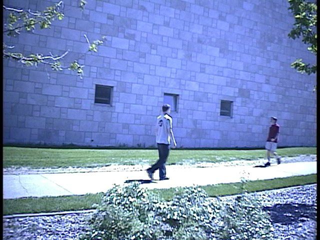
Typical situations the system should handle include sume that these points represent the head, hands and feet.
people walking parallel to or facing the camera (see fig- The exact position of the body parts is not required for
ure 2). However, the system must be robust and toler- their application. In the second class, involving systems
ate more complex situations. The main assumption to be which provide the exact position of all body joints, one
made is that people shall be in an upright position. can find [6], which uses a stick-model and tries to fit it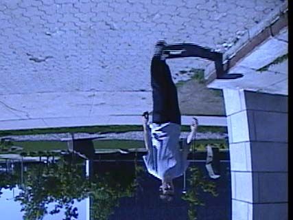
Division of the
                                                                           bounding box
                                                                            in four sub-
                                                                             bounding
                                                                                boxes
                                          Blobs
    Background      Background                                                                                              Fitting of the
                                        extraction
     modeling       subtraction                                                                                              four limbs
                                       and dilation

                                                        Computation of      Determination         Scaling and
                                                         the distance        of the trunk        positionning of
                                                           transform         extremities            the torso

                                               Figure 1: Overview of the system.

to the blob. Neural networks [13] and genetic algorithms          is computed for the whole blob. Then the blob is divided
[12] are also used. Finally, [4] presents a method dealing        in four sections by tracing vertical and horizontal lines
specifically with the detection of armed robbery. This            through the center of mass. The new bounding boxes are
method analyses the skeletonization of the blob to decide         computed for each of the four sub-images. These four
whether or not a robbery is taking place in the scene.            bounding boxes will serve in the limbs fitting module.
    The interest of the method described herein is that it
combines, in the same system, the speed of some tech-
niques and the robustness of others, while giving a com-
plete description of the body. These three elements are
almost never present simultaneoustly in a system.

3      Proposed approach
                                                                                a)                                     b)
A general overview of the system is presented in 1.
                                                                  Figure 2: a) Typical situation the system has to handle. b)
                                                                  Blobs extraction before any treatment.
3.1     Blobs Extraction
A custom background subtraction method is used to ex-
tract the silhouette of the person. That is, the mean and
the standard deviation of each pixel is computed in a se-
ries of images without any person. Then, a pixel is re-
garded as belonging to a moving object if the difference
between the mean and the current value of that pixel is
higher than a certain threshold related to the standard de-
viation. Figure 2 b) shows background subtraction.
    Once this step is completed, a test is made on each of
the blobs obtained to ensure that the area is sufficient, and
not composed only of noise. Blobs which are too small                           a)                                     b)
are eliminated. A filling algorithm is then used to ensure
that the blobs are exempt of any holes. Finally, two steps        Figure 3: a) A binary blob and the four corresponding bound-
of dilation are carried out to obtain a smooth silhouette.        ing boxes. b) The distance transform obtained for image a) and
    Then, a distance transform is computed on this image,         normalized between 0 and 255.
using an implementation of the two pass algorithm [3].
The result, shown in figure 3, is an image which gives,
for each pixel, the distance from the nearest contour. This       3.2    Skeleton model
result is used in further processing.
    In our method, the fitting is carried out progressively,      The skeleton model used herein is represented by a vector
one limb at a time. It is necessary to ensure that each limb      of 14 body parts. It is shown in figure 4.
covers his part of the blob. This is why the bounding box
is divided into four parts. To do this, the center of mass                           B = {bp1 , bp2 , . . . , bp14 }                         (1)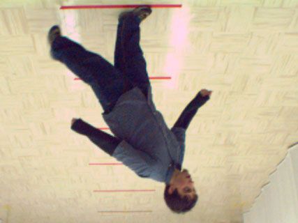
bp1                                                                 blob and finding the maximum of the distance transform
                                                              bp1                 for each of the sampled points. Using linear regression,
              bp2    bp5
                                         ex2,2=ex3,1                              a line is fitted on the points sampled, and the height is
        bp3                bp6                                ex2,1=ex1,2
                                                       bp2                        found by raising a segment up following the line direction
                    bp8                                                           until the blob’s frontiers are reached.
      bp4                  bp7           bp3
                                                                                      Let DT be the distance transform image. DT(x,y)
              bp9 bp12
                                               ex3,2=ex4,1
                                                                                  would be the value (between 0 and 255) of the pixel at
                                                              bp8
         bp10         bp13                                                        coordinate (x,y) in the distance transform image. The first
                                                                                  extremity of the trunk is ex8,1 = (x8,1 , y8,1 ). y8,1 is set
                                         bp4
                                                                                  constant to 2/15 of the person’s height and x8,1 is com-
         bp11         bp14
                                                                                  puted as being the pixel that maximize the value of the
                                                        bp9     bp12
                                                                                  distance transform. Let xl be the left x coordinate of the
                a)                                      a)                        bounding box, and xr be the right coordinate. We can
                                                                                  compute
Figure 4: a) The stick-model used to do the fitting. b) A closer
look at the right arm.                                                                         x8,1 = x| max (DT (i, y8,1 ))                (5)
                                                                                                          xl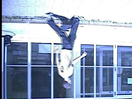
Figure 5: Torso fitting. The lenght of the torso is defined based   Figure 6: One particular position for bp3 and all the candidate
on the blob’s size. Then the torso model is scaled and his po-      positions generated by the system for bp4 . This process is re-
sition is determined using an algorithm based on the distance       peated for all possible positions of bp3 admitted by the angle
transform.                                                          constraints. The sampling angle in this case is π/32.

fixed as having the same coordinates as exi−1,2 (these co-          image:
ordinates are known because exi−1,2 belongs to the torso
                                                                                   n                    m
and the torso has already been fitted). Then, the set S                            X                    X
                                                                         IRiαβ =         DT (pα
                                                                                              k,i ) +         DT (pβk,i+1 )   (10)
of all candidate solutions for this limb is generated. In
                                                                                   k=1                  k=1
other words, all the possible positions for bpi and bpi+1
are generated according to the angle constraints that were          where DT (pα                                   α
                                                                                  k,i ) is the value of the pixel pk,i in the dis-
imposed, and with a predefined sampling angle (see fig-             tance transform image.
ure 6). This angle influences the robustness and speed of               The greater the distance between the limb and any
the technique. If the sampling angle is too large, a good           contour, the highest the IR value is.
solution could be overlooked. However, the whole pro-                   The second criterion is the coverage rating (CR),
cess might be too long if the sampling angle is chosen              which is related to the bounding box. It is a boolean vari-
small. It then becomes possible to sample points along              able. Since the bounding box has been divided into four
bpi and bpi+1 for each candidate solution. For a particu-           parts, there is one CR for every limb. When Li is fitted,
lar solution, if the angle between bpi−1 and bpi is α and           a test is processed to ensure that the blob is covered, i.e.
angle between bpi and bpi+1 is β, these sampled points              ex2i+1 is close enough from the limb’s bounding box. If
are                                                                 so, CR takes the value true. Otherwise, it assumes the
                                                                    value false. At this point, the minimal distance to fix the
                                                                    CR criterion as true has been set to 10% of the person’s
                    Piα = {pα              α
                            1,i , . . . , pn,i }             (8)
                                                                    height. If CR is true, the solution is accepted and the
             β
            Pi+1   =   {pβ1,i+1 , . . . , pβm,i+1 }          (9)    corresponding IR value is compared to those of the other
                                                                    potential solutions. The solution meeting the CR crite-
where pα 1,i is the coordinate of the first sampled point of        rion and having the highest IR is considered as being the
the body part bpi in the candidate solution with angle α.           best solution.
Here n and m depend on the sampling rate. The sampling
rate is an adjustable parameter that also influences the
robustness and speed of the method. Indeed, the more                4    Strength
points there are along a line to validate a solution, the
more robust the system is if a part of a limb has been              This method is fast compared to a global fitting method.
poorly extracted. However, the more time-consuming the              The whole process takes about one second on a Pentium
fitting process becomes.                                            III 550MHz. The fact that all limbs are fitted indepen-
     Two criteria have been developed which determine if            dently of each other speeds-up the process and avoids
a solution is good or not. The first one is the interior rat-       the combinatorial complexity problem which would oc-
ing (IR), which is computed with the distance transform             cur with a global method.
houettes are between 137 and 320 pixels high. For a blob
                                                                  with defaults (shadow, incomplete parts, etc.), the local
                                                                  fitting method permits in most cases to obtain satisfac-
                                                                  tory results, at least for the body parts that have been cor-
                                                                  rectly extracted. Figure 9 shows that the method is able to
                                                                  process blobs that are not well shaped, for instance more
                                                                  difficult cases with different kinds of shadows.
                                                                      An evaluation technique to analyse the results has
                                                                  been developed to classify a given solution for a partic-
              a)                             b)                   ular blob as being either acceptable or not by comparing
                                                                  how the stick-model has been fitted to a blob by the sys-
                                                                  tem and by humans. First, the skeleton is fitted by the
                                                                  computer and the joints of the skeleton are saved. The
                                                                  same blob is then fitted by a human. This is considered
                                                                  as the optimal solution. To compare these two solutions,
                                                                  the distance between each of the main joints is computed.
                                                                  This distance is then normalized to compensate for the
                                                                  scale effect. The results presented herein are for a trunk
                                                                  of 100 pixels. Mean and standard deviations shown in ta-
              c)                             d)                   ble 1 have been determined for 500 silhouettes. Table 2
                                                                  presents results for the 10 best fitted skeletons and table
Figure 7: Limbs fitting. Fitting is done independently for each   3 gives results for average fitted skeleton. Finally, table 4
limb. This local method speeds up the process and improves
                                                                  shows results for poorly fitted skeletons.
the robustness if some regions of the blob have been poorly ex-
tracted.                                                              Experiments show that an error of less than 5 pixels
                                                                  for a joint is excellent and that an error of about 10 pixels
                                                                  is acceptable. The reader will notice that poor fitting is
    This method also facilitates the segmentation of the
                                                                  mainly due to scaling errors, i.e. the height of the blob has
body into different parts. Indeed, the system does not
                                                                  not been correctly determined, and to unusual positions,
only extract the position of an extremity (a hand or a
                                                                  for example if a limb is not visible in the image. However,
foot, for example), but rather a segment that represents
                                                                  because of the local fitting method, even if one part is
the whole limb. This element will be very useful when
                                                                  missed, the overall fitting is often acceptable.
the pixels representing this limb must be extracted. A
system which only provides the extremity position does
not give any indication as to where the limb connected to
this extremity is located.
    A local method such as the one presented here also
increases the robustness of the whole system in the fol-
lowing way. If some region of the blob has been poorly
extracted, it is likely that only this part will be poorly fit-
ted and that the other limbs will be succesfully fitted, at
least if the torso has been successfully fitted. In the case
of a global method, a small error can lead to the failure
of the whole fitting module.

5    Experimental results
The different modules of the system have been tested on
a series of 500 images. These blobs represent silhou-
ettes with varying scales, point of vues, standing poses
(including poses where the head does not represent the            Figure 8: The segmentation of the body in his different parts
                                                                  is the next step toward building an operational and efficient sys-
highest point of the blob or where the person is bending)
                                                                  tem.
and levels of precision in the blob extraction.
    Tested images have 640x480 pixels and typical sil-
6    Conclusion                                                  [5] H. Fujiyoshi and A. Lipton. Real-time human mo-
                                                                     tion analysis by image skeletonization. In Proceed-
In this paper, a new method of stick-model or skeleton fit-          ings of the 4th IEEE Workshop on Applications of
ting has been presented. This technique is original in that          Computer Vison, pages 15–21, 1998.
it is performed progressively, one limb at a time, instead
of globally. This way, the process is faster. A skeleton         [6] Yan Guo, Gang Xu, and Saburo Tsuji. Understand-
model was defined and scaled with respect to the person’s            ing human motion patterns. In Proceedings of the
height. However, the blob’s height does not always rep-              12th International Conference on Pattern Recogni-
resents the person’s height and this could lead to an error          tion, pages 325–330, 1994.
in the scaling factor. To overcome this problem, an algo-        [7] I. Haritaoglu, D. Harwood, and L. Davis. Who,
rithm was developed to compute the height of the person              when, where, what: A real time system for detect-
even in situations where the head is not the highest point           ing and tracking people. In Proceedings of the 3th
of the blob.                                                         Face and Gesture Recognition Conference, pages
     The four limbs of the model are scaled with respect to          222–227, 1998.
the torso size. Then, they are fitted individually by gener-
ating all possible positions and selecting the best position.    [8] L. Herda, P. Fua, R. Plankers, R. Boulic, and
This best solution is computed using two criteria. First,            D. Thalmann. Skeleton-based motion capture for
the IR criterion gives a measure of the depth of a limb in a         robust reconstruction of human motion. In Pro-
blob, i.e. how far the limb is located from any contour, by          ceedings of the Computer Animation, pages 77–83,
using the distance transform of the blob’s binary image.             2000.
The CR criterion then involves the validation of the posi-
                                                                 [9] S. Ioffe and D. Forsyth. Finding people by sam-
tion of the limb by checking if the limb covers the total
                                                                     pling. In Proceedings of the 7th International Con-
bounding box area. As the fitting is conducted separately
                                                                     ference on Computer Vision, volume 2, pages 1092–
for each limb, a different bounding box is computed for
                                                                     1097, 1999.
each part of the blob.
     Future work includes segmenting the person into dif-       [10] Anuj Mohan, Constantine Papageorgiou, and
ferent parts (see figure 8) as well as possibly improving            Tomaso Poggio. Example-based object detection in
the system by adding a module to analyse the posture of              images by components. IEEE Transactions on Pat-
the subject based on the skeleton position.                          tern Analysis and Machine Intelligence, 23(4):349–
Acknowledgements: This research was supported by an                  361, 2001.
NSERC grant to R. Bergevin.
                                                                [11] NASA. Anthropometric Source Book, volume 2.
                                                                     Springfield VA, Johnson Space Center, Houston,
References                                                           TX, 1978.
                                                                [12] Jun Ohya and Fumio Kishino. Human posture es-
 [1] Norman I. Badler, Cary B. Phillips, and Bon-                    timation from multiple images using genetic algo-
     nie Lynn Webber. Simulating Humans: Computer                    rithm. In Proceedings of the 12th International
     Graphics Animation and Control. Oxford Univer-                  Conference on Pattern Recognition, pages 750–753,
     sity Press, New York, 1993. ISBN 0-19-507359-2.                 1994.
 [2] Carlos Barrón and Ioannis A. Kakadiaris. Estimat-         [13] Kazuhiko Takahashi, Tetsuya Uemura, and Jun
     ing anthropometry and pose from a single uncali-                Ohya. Neural-network-based real-time human body
     brated image. Computer Vision and Image Under-                  posture estimation. In Proceedings of the 2000
     standing: CVIU, 81(3):269–284, march 2001.                      IEEE Signal Processing Society Workshop, vol-
                                                                     ume 2, pages 477–486, 2000.
 [3] Gunilla Borgefors. Distance transformations in dig-
     ital images. Computer Vision, Graphics, and Image
     Processing, 34(3):344–371, june 1986.

 [4] Jaime Dever, Niels da VitoriaLobo, and Mubarak
     Shah. Automatic visual recognition of armed rob-
     bery. In Proceedings of the 16th IEEE Inter-
     national Conference on Pattern Recognition, vol-
     ume 1, pages 451–455, 2002.
Stats    Head        Upper    Right    Right      Left      Left     Lower      Right     Right      Left      Left      Global
                       Trunk    Elbow    Hand      Elbow      Hand     Trunk      Knee      Foot       Knee      Foot
   µ        9.32        8.40    13.22    16.67      9.41     10.33     10.40      16.17     15.51     15.43     15.51      12.76
   σ        9.58       10.20    15.70    30.63      7.30      8.05      8.01       8.58      8.79      8.50      8.79      7.66

Table 1: Mean difference (µ) and Standard deviation (σ) for the 500 images. The distance is computed in pixels and normalized
for a trunk of 100 pixels. The Global column represents the mean of all distances.

  ID       Head        Upper    Right    Right      Left      Left     Lower      Right     Right      Left      Left      Global
                       Trunk    Elbow    Hand      Elbow      Hand     Trunk      Knee      Foot       Knee      Foot
  406       3.34         2.11    1.49     2.11      4.72       5.38     6.67       6.33      1.49     10.55       1.49     4.15
  295       2.31         5.17    3.27     4.90      1.63       4.62     0.00      13.96      1.63      6.74       1.63     4.17
  164       6.56         1.82    3.64     5.75      4.07       6.56     4.07       7.71      4.07      4.07       4.07     4.76
  297       1.61         4.82    3.21     6.81      6.81       2.27     3.59      18.79      1.61      7.18       1.61     5.30
  475       5.02         1.22    0.00     6.56      4.39       6.09     1.72       8.18      8.18      9.83       8.18     5.40
  236       7.93         3.55    3.55    10.64      5.72       8.09     1.59       7.93      4.49      1.59       4.49     5.41
  381       3.15         2.81    1.41     4.45      5.07       3.98     8.56       8.90      7.96      5.80       7.96     5.46
  403       4.94         1.56    3.13     4.94      6.25       9.38     7.97       6.99      3.49      9.50       3.49     5.60
  301       3.65         4.61    3.26     6.73      0.00       4.61     7.30      12.42      3.65     11.88       3.65     5.61
  410       5.65         1.94    4.94     3.06      3.06       3.06    10.96       8.33      4.94     12.63       4.94     5.77

Table 2: The difference for joint location for the ten skeletons with the best fitting. The distance is computed in pixels and
normalized for a trunk of 100 pixels. The ID column represents the frame number and some results presented herein can be
referenced in figure 9.

  ID       Head        Upper    Right    Right      Left      Left     Lower      Right     Right      Left      Left      Global
                       Trunk    Elbow    Hand      Elbow      Hand     Trunk      Knee      Foot       Knee      Foot
  207       5.17         5.45   12.06     6.89     11.56     11.56       5.45     16.97     12.06     11.56     12.06      10.07
  307       3.72         6.00   30.15    29.50      6.00      6.86       5.26     10.13      4.99      3.33      4.99      10.09
  316       6.64         5.81   10.81    14.85      6.83      8.06       1.61     11.73     14.41     16.11     14.41      10.12
  152       6.67         5.85    6.67     6.67      0.00      9.25       3.70     14.45     21.10     15.81     21.10      10.12
  651       9.82         6.09   16.69    32.90      5.81      5.29       6.61      8.37     13.41     11.56     13.41      11.81

Table 3: The difference for joint location for skeletons with average fitting. The distance is computed in pixels and normalized for
a trunk of 100 pixels.

  ID       Head        Upper    Right    Right      Left      Left     Lower      Right     Right      Left      Left      Global
                       Trunk    Elbow    Hand      Elbow      Hand     Trunk      Knee      Foot       Knee      Foot
  461     52.28        36.28    74.24   157.59     26.74      2.05     18.57      16.41      4.35     13.37      4.35      36.93
  350     50.52        52.34    44.89   29.72      68.85     91.97     20.39      19.37     10.75     10.75     10.75      37.30
  501     31.50        42.15    50.83   34.69      28.10     21.51     50.37      55.04     53.22     53.72     53.22      43.12
  131     27.41        29.59    64.10   152.37     28.16     27.79     14.40      19.58     41.04     33.61     41.04      43.55
  132     33.98        33.98    61.53   150.00     36.52     30.81     30.81      35.16     36.52     36.52     36.52      47.49

Table 4: The difference for joint location for skeletons with poor fitting. The distance is computed in pixels and normalized for a
trunk of 100 pixels.
a)164                          b)164                          c)295                          d)295

           e)381                          f )381                         g)406                          h)406

            i)475                         j)475                          k)651                          l)651

           m)131                          n)131                          o)350                          p)350

             q)                             r)                             s)                             t)

Figure 9: Some results obtained with the described method. First and third columns represent the original images,
second and fourth columns represent the fitted skeleton. Figures a) to j) show very good results obtained in different
situations. Figures k) and l) are an average fitted skeleton. Shoulders are a bit too large, but the scale factor is the
good one and the overall fitting is acceptable. Figures m) to p) present poor fitting. In these two cases, the height is
not the good one, which leads to scaling error. This is due to the head position. However, the overall fitting is still not
so bad. Finally, figures q) to t) demonstrates, with images took in different conditions, that using the bounding box
constraints, the skeleton is well fitted even if there is shadow between the two legs (r) or side shadow (t).
You can also read