The photosphere/corona interface: new perspectives

The photosphere/corona interface:
              new perspectives
Philip Judge + R. Centeno, M. Kubo, B. Lites, S.
McIntosh, A. G. de Wijn, HAO; G. Cauzzi, K.
Reardon, Arcetri; A. Tritschler, H. Uitenbroek NSO

re-visiting some physical issues
     old vs. new perspectives
     magnetic interface
     thermal interface
                                                        September 2008

               The National Center for Atmospheric Research is operated by the University Corporation for Atmospheric Research
                  under sponsorship of the National Science Foundation. An Equal Opportunity/Affirmative Action Employer.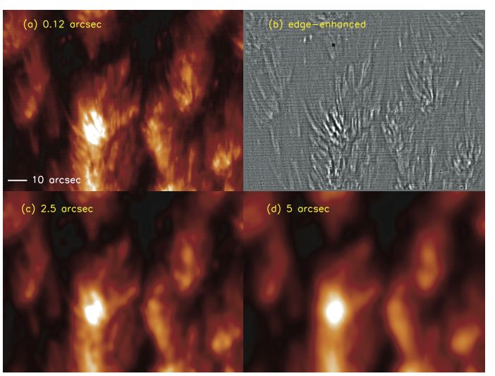

the chromosphere

•   stratified: spans 9 pressure scale heights
•   requires 30-100x as much power as the corona
•   usually contains plasma =1 surface
•   is the lower boundary for the corona
    – modulates flow of mass, momentum, energy and
      magnetic field into the corona
    – implicit mass reservoir in coronal loop scaling laws
• yet
    – “chromosphere Hinode” search reveals 1/3 of
      “corona Hinode” publications
    – chromosphere is an “ignore-o-sphere”?
    – “too complicated”?

Example of “old” perspectives
SKYLAB data - VAL thermal models

                      1D
                      RT
                      nLTE
                      HSE
                      PRD
                      ...

Heroic reference work of vital importance, 1981

Recent(!) example of “old” perspectives
     nlff field extrapolation (Schrijver et al 2008)
red:
current

          Hinode SP photospheric vector polarimetry, no
          chromospheric data (nb. Low & Flyer 2007)

New perspectives: DOT and TRACE
       9 Jul 2005 (A.G. de Wijn, R. J. Rutten)

photosphere
chromosphere
corona

magnetic interface

Magnetism and the solar atmosphere
                               lower corona     upper
                                                chromosphere
• measure B where possible
• high plasma conductivity-
  “trace field lines” from
  photosphere to corona
• TRACE & other missions
  failed to do this
• why?- chromosphere

          De Pontieu et al. 1999 upper          magnetic elements +
          “moss”                 chromosphere   reverse granulation

Gold (1964)
• consider potential
  and f-f fields in
  upper half
• the electro-
  dynamics of the
  chromosphere is
  critical to the
  supply of
  magnetic free
  energy into the
  corona.
• traditionally it is
  treated as in the
  figure

magnetic interface
  observations:
   an example

Small AR, pores

Small AR, pores: closer view

Chromosphere as seen with IBIS
• Ca II 854.2 nm
• samples many pressure
  scale heights

• base of corona is very
  different from
  photosphere

                           G. Cauzzi et al 2008, A+A

Small AR, pores: high resoution
photosphere and chromosphere

detailed study of IBIS data: G. Cauzzi et al 2008, A+A

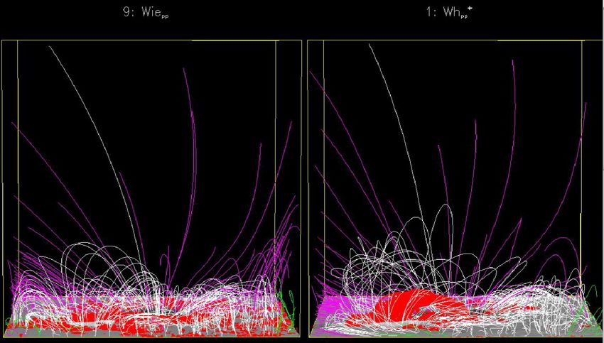
Differences between potential
           and constant α photospheric fields
• IBIS morphology⇒ transverse
  fields differ by ~20-40G
• Hinode 630.2 sensitivity BT(app)
  Lites et al (2008) ApJ 672, 1237
   – 40 Mx cm-2 px-1 (normal map)
   – 20 Mx cm-2 px-1 (deep map)
• Hinode can study photospheric vs
  chromospheric electrical currents,
  forced ➔ force free transition!
• Total ÷ potential energy:
   – 2 (chromosphere)
   – 5-10 (corona)

Hale 1908: 100 years on

                     Inspiration for
                     much work
                     generically
                     called
                     “chromospheric
                     fine structure”

magnetic interface
physical considerations

Note: twist/ electrical currents can be easier to
              detect in the chromosphere!
• IBIS again: clear Bφ ⇒ jz
• Hinode rotating spicules
• ang. mom. conservation around tubes
• Knölker et. al. (1988)- tube
  stability requires rotating flow

• Parker (1974): Bφ/Bz increases with z

Chromosphere vs. photosphere
                as the coronal boundary
• chromosphere spans 9 scale heights
• ⇒ chromosphere usually contains β=1 surface
   – j×B→ β B2/2µ above β=1 j⊥ → small
• partial ionizn⇒ 3-fluid frictional dissipation, heating
   – Qfr = j2/σ + (ξn j×B - G)2/αn,      G = ξn ∇p - ∇pn
   – “ambipolar diffusion”/star formation (1950s Schlüter, Cowling)
• case G = 0 ⇒ “Cowling conductivity” σ⊥* (Arber & cohorts)
   – Qfr = jǁ2/σ + j⊥2/σ⊥* σ /σ⊥*= 1 + 2 ξn ϖeτe ϖiτi >>1
   – ⇒ dissipation of j⊥. Explains why IBIS nearly f-f?
• NOTE: σ⊥* is some steps removed from σ (kinetic theory)
   – case G ≠ 0: σ⊥* incorrect!
   – one must simultaneously determine the nature of j⊥ (cf. E-region
     electrojet) from the dynamics

Chromosphere tends to “filter out” j⊥ : coronal
       base magnetic field → force-free
                                     Flux emergence: Arber, Haynes &
• Braginskii (1965): certain         Leake (2007) based upon Cowlingʼs
  motions (G...) dissipate j⊥        conductivity (G=0):
   – Alfvén, fast modes, dynamic
     situations where
     ∇p - ρg + j×B ≠ 0
• Not slow modes, slow
  dynamics (cf. Goodman 2000)
• So, at coronal lower boundary,
  chromosphere makes:
   – j⊥∼0; j×B∼0
   – weaker Alfvén/fast modes               ...radical effect on flux
   – curl B = αB: α(r) → constant?          emergence process
   –       (Parker current sheets..)

thermal interface

The problem- observations
• Feldman and colleagues (1983-)
   – different morphology 104 -106 K, other properties
   – TR thermally, magnetically isolated from the corona
   – radiating entity = “unresolved fine structures”

Dowdy et al. (1986)

• Mixed polarity
  within network
  boundaries
• tries to explain
  “UFS”
• indeed these are
  thermally and
  magnetically
  separate entities

Depontieu et al 2003: TRACE/SST data

Yet...

Significant correlations
exist between the H
chromospheric intensity
and the low corona

Questions concerning cool loops
• Cool loops are considered by most a viable
  explanation, but
• where does the 106 erg cm-2 s-1 conductive
  flux go?
• Is it merely a coincidence that the lower TR
  radiates about 106 erg cm-2 s-1?
• Why should the cool loop distribution make the
  upper (conductive) and lower (cool loop) TR be
  correlated, at least on scales > a few Mm?
• are they stable (Cally & Robb 1991)?
• where are the tell-tale magnetic footpoints?
• ...

Judge & Centeno (2008)

• VAULT L data vs.
  KPNO magnetic data
                              Patsourakos et al:
   – supplemented by
     Hinode SP vector
     polarimetry
• Prompted by
  Patsourakos et al
  (2007)
   – We noted something
     “odd” about
     proposed cool loops
   – large-scale alignment
     of L threads

KPVT+POTL FIELDS+VAULT
                      active network
Black=low-lying loops (h

Spicules, fibrils..

• base of the corona is a
  non-planar thermal
  boundary
• e.g., DOT H (Rutten
  2007) clockwise 0, -0.4,
  -0.6,-0.8 Å:

  consider α in
  curl B = αB for photosphere
  and coronal base

Hinode spicules

• Ca II (radial filter to enhance spicules, M. Carlsson)
spicules arise
from within
the chromo-
sphere

stratified VAL
chromosphere
1.5Mm only

Judge (2008) ApJL 683, 87-90
“spicule” ➜ cross field diffusion➜ TR radiation

Results: model L ~0.1x observed
               using only local coronal heat
1D 3-fluid
calculation
of cross-field
diffusion
from a cool
flux tube into
coronal
plasma

no field
aligned
conduction

           calculations with different coronal n,T: non-linear
           relationship between L and coronal emission

Judge (2008)

• calculations for L are promising, (also L, He I 584)
   – this is the hardest line to explain, others may follow?
• cross-field diffusion of neutrals might solve the 40+ yr problem
  of energy balance in extended structures in the lower TR
• chromosphere supplies the mass, corona the energy
   – cool loops don’t explain active network (Judge & Centeno 2008)
   – “UFS” in this new picture is thermally connected to the corona

• needed
   – 2D calculations including field-aligned conduction and dynamics
   – observations of the chromosphere/corona interface in relation to
     magnetic field

Conclusions
• the magnetic chromosphere remains poorly understood
• the Sun undergoes the awkward transition from forced β>1 to force-
  free β

To understand the corona we must understand what is under
       Gold’s line... is single-fluid MHD adequate?