Real Time Distributed Stock Market Forecasting using Feed-Forward Neural Networks, Market Orders, and Financial indicators
←
→
Page content transcription
If your browser does not render page correctly, please read the page content below
Real Time Distributed Stock Market
Forecasting using Feed-Forward Neural
Networks, Market Orders, and Financial
indicators

A distributed multi-model approach to stock forecasting

Master’s thesis in Computer science and engineering

Oscar Carlsson, Kevin Rudnick

Department of Computer Science and Engineering
C HALMERS U NIVERSITY OF T ECHNOLOGY
U NIVERSITY OF G OTHENBURG
Gothenburg, Sweden 2021

Master’s thesis 2021

      Real Time Distributed Stock Market
Forecasting using Feed-Forward Neural Networks,
    Market Orders, and Financial indicators

    A distributed multi-model approach to stock forecasting

                Oscar Carlsson, Kevin Rudnick

          Department of Computer Science and Engineering
            Chalmers University of Technology
                 University of Gothenburg
                    Gothenburg, Sweden 2021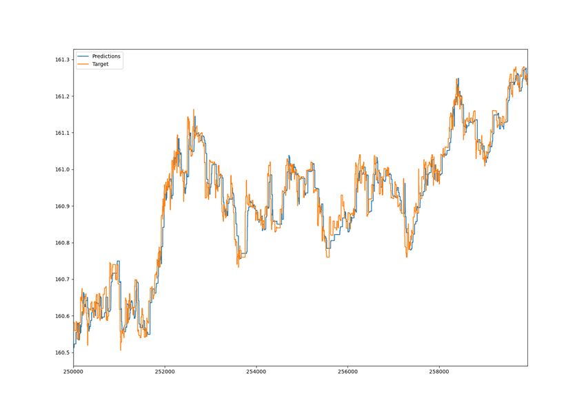
Real Time Distributed Stock Market Forecasting using Feed-Forward Neural Net-
works, Market Orders, and Financial indicators
A distributed multi-model approach to stock forecasting
Oscar Carlsson, Kevin Rudnick

© Oscar Carlsson, Kevin Rudnick, 2021.

Supervisor: Philippas, Tsigas
Examiner: Andrei, Sabelfeld

Master’s Thesis 2021
Department of Computer Science and Engineering
Chalmers University of Technology and University of Gothenburg
SE-412 96 Gothenburg
Telephone +46 31 772 1000

Typeset in LATEX
Gothenburg, Sweden 2021

iv

Real Time Distributed Stock Market Forecasting using Feed-Forward Neural Net-
works, Market Orders, and Financial indicators
A distributed multi-model approach to stock forecasting
Oscar Carlsson, Kevin Rudnick
Department of Computer Science and Engineering
Chalmers University of Technology and University of Gothenburg

Abstract
Machine learning and mathematical models are two tools used in prior research of
stock predictions. However, the stock market provides enormous data sets, making
machine learning an expensive and slow task, and a solution to this is to distribute
the computations. The input to the machine learning in this thesis uses market
orders, which is a different way to make short-term predictions than previous work.
Distributing machine learning in a modular configuration is also implemented in
this thesis, showing a new way to combine predictions from multiple models. The
models are tested with different parameters, with an input base consisting of a list of
the latest market orders for a stock. The distributed system is divided into so-called
node-boxes and tested based on latency. The distributed system works well and has
the potential to be used in large systems. Unfortunately, making predictions with
market orders in neural networks does not provide good enough performance to be
viable. Using a combination of predictions and financial indicators, however, shows
better results.

Keywords: Machine learning, deep neural network, distributed systems, stock mar-
ket prediction, market orders.

                                                                                     v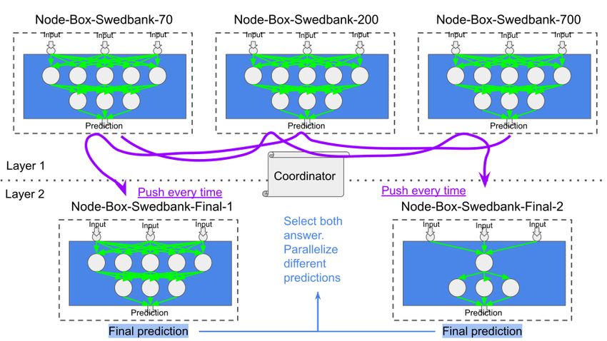
Acknowledgements
We would like to thank our supervisor Philippas Tsigas for the guidance, support,
and advice during the thesis.

We would also like to thank our examiner Andrei Sabelfeld for taking the time to
read trough our thesis and giving us feedback.

Finally we want thank our partners-in-life Amanda and Sonja for supporting us
throughout this thesis and always keeping spirits high. Long live beters.

                          Oscar Carlsson, Kevin Rudnick, Gothenburg, June 2021

                                                                              vii
Contents

List of Figures                                                                                                                xiii

List of Tables                                                                                                                 xvii

1 Introduction                                                                                                                   1
  1.1 Aim of The Project . . . . . . .     .   .   .   .   .   .   .   .   .   .   .   .   .   .   .   .   .   .   .   .   .     2
  1.2 Risk and Ethical Considerations      .   .   .   .   .   .   .   .   .   .   .   .   .   .   .   .   .   .   .   .   .     2
  1.3 Limitations . . . . . . . . . . .    .   .   .   .   .   .   .   .   .   .   .   .   .   .   .   .   .   .   .   .   .     3
  1.4 Thesis outline . . . . . . . . . .   .   .   .   .   .   .   .   .   .   .   .   .   .   .   .   .   .   .   .   .   .     3

2 Theory                                                                                                                         5
  2.1 Stock market momentum . . . . . . . . . . . . .                          .   .   .   .   .   .   .   .   .   .   .   .     5
  2.2 Lagging and leading indicators . . . . . . . . . .                       .   .   .   .   .   .   .   .   .   .   .   .     5
      2.2.1 Exponentially weighted moving average .                            .   .   .   .   .   .   .   .   .   .   .   .     5
      2.2.2 Relative Strength Index . . . . . . . . .                          .   .   .   .   .   .   .   .   .   .   .   .     6
      2.2.3 Moving Average Convergence Divergence                              .   .   .   .   .   .   .   .   .   .   .   .     6
      2.2.4 Volatility . . . . . . . . . . . . . . . . .                       .   .   .   .   .   .   .   .   .   .   .   .     7
      2.2.5 Price Channels . . . . . . . . . . . . . .                         .   .   .   .   .   .   .   .   .   .   .   .     7
  2.3 Machine Learning . . . . . . . . . . . . . . . . .                       .   .   .   .   .   .   .   .   .   .   .   .     7
      2.3.1 Neural networks . . . . . . . . . . . . . .                        .   .   .   .   .   .   .   .   .   .   .   .     7
      2.3.2 Loss function . . . . . . . . . . . . . . .                        .   .   .   .   .   .   .   .   .   .   .   .     8
             2.3.2.1 Backpropagation . . . . . . . .                           .   .   .   .   .   .   .   .   .   .   .   .     9
      2.3.3 Activation functions . . . . . . . . . . .                         .   .   .   .   .   .   .   .   .   .   .   .    10
             2.3.3.1 ReLU . . . . . . . . . . . . . .                          .   .   .   .   .   .   .   .   .   .   .   .    10
             2.3.3.2 Leaky ReLU . . . . . . . . . .                            .   .   .   .   .   .   .   .   .   .   .   .    10
  2.4 Normalization . . . . . . . . . . . . . . . . . . .                      .   .   .   .   .   .   .   .   .   .   .   .    10
      2.4.1 Min-max Normalization . . . . . . . . .                            .   .   .   .   .   .   .   .   .   .   .   .    11
      2.4.2 Z-Score Normalization . . . . . . . . . .                          .   .   .   .   .   .   .   .   .   .   .   .    11

3 Previous work                                                                                                                 13

4 Methods                                                                                                                       15
  4.1 Data . . . . . . . . . . . . . . . . . .         .   .   .   .   .   .   .   .   .   .   .   .   .   .   .   .   .   .    15
      4.1.1 Building features . . . . . . .            .   .   .   .   .   .   .   .   .   .   .   .   .   .   .   .   .   .    15
            4.1.1.1 Price . . . . . . . . .            .   .   .   .   .   .   .   .   .   .   .   .   .   .   .   .   .   .    15
            4.1.1.2 Time . . . . . . . . .             .   .   .   .   .   .   .   .   .   .   .   .   .   .   .   .   .   .    15
            4.1.1.3 Financial indicators               .   .   .   .   .   .   .   .   .   .   .   .   .   .   .   .   .   .    16

                                                                                                                                 ix
Contents

          4.1.2 Matching x and y data . . . . .       .   .   .   .   .   .   .   .   .   .   .   .   .   .   .   .   .   16
          4.1.3 Graphs . . . . . . . . . . . . . .    .   .   .   .   .   .   .   .   .   .   .   .   .   .   .   .   .   17
    4.2   Distributed system . . . . . . . . . . .    .   .   .   .   .   .   .   .   .   .   .   .   .   .   .   .   .   17
          4.2.1 Node-Box . . . . . . . . . . . .      .   .   .   .   .   .   .   .   .   .   .   .   .   .   .   .   .   17
          4.2.2 Smart-sync . . . . . . . . . . .      .   .   .   .   .   .   .   .   .   .   .   .   .   .   .   .   .   18
          4.2.3 Applying Techniques in Layer 1        .   .   .   .   .   .   .   .   .   .   .   .   .   .   .   .   .   21
          4.2.4 Coordinator . . . . . . . . . . .     .   .   .   .   .   .   .   .   .   .   .   .   .   .   .   .   .   21
          4.2.5 Coordinator Protocol . . . . . .      .   .   .   .   .   .   .   .   .   .   .   .   .   .   .   .   .   21
          4.2.6 Redundancy . . . . . . . . . . .      .   .   .   .   .   .   .   .   .   .   .   .   .   .   .   .   .   23
          4.2.7 Parallelization . . . . . . . . . .   .   .   .   .   .   .   .   .   .   .   .   .   .   .   .   .   .   23
          4.2.8 Cycling node-boxes . . . . . . .      .   .   .   .   .   .   .   .   .   .   .   .   .   .   .   .   .   23
          4.2.9 Financial Indicator Node . . . .      .   .   .   .   .   .   .   .   .   .   .   .   .   .   .   .   .   24
          4.2.10 Test Bench . . . . . . . . . . .     .   .   .   .   .   .   .   .   .   .   .   .   .   .   .   .   .   25
    4.3   Stock predictor . . . . . . . . . . . . .   .   .   .   .   .   .   .   .   .   .   .   .   .   .   .   .   .   25
          4.3.1 PyTorch . . . . . . . . . . . . .     .   .   .   .   .   .   .   .   .   .   .   .   .   .   .   .   .   25
          4.3.2 Neural networks . . . . . . . . .     .   .   .   .   .   .   .   .   .   .   .   .   .   .   .   .   .   26
          4.3.3 Input data . . . . . . . . . . . .    .   .   .   .   .   .   .   .   .   .   .   .   .   .   .   .   .   26
          4.3.4 Output data . . . . . . . . . . .     .   .   .   .   .   .   .   .   .   .   .   .   .   .   .   .   .   27
          4.3.5 Training . . . . . . . . . . . . .    .   .   .   .   .   .   .   .   .   .   .   .   .   .   .   .   .   28
          4.3.6 Testing . . . . . . . . . . . . . .   .   .   .   .   .   .   .   .   .   .   .   .   .   .   .   .   .   28

5 Results                                                                                                                 31
  5.1 Feed-forward Neural Network . . . . . . . . . . . .                         . . . .         .   .   .   .   .   .   31
      5.1.1 Min-max normalization . . . . . . . . . . . .                         . . . .         .   .   .   .   .   .   31
      5.1.2 Z-normalization . . . . . . . . . . . . . . . .                       . . . .         .   .   .   .   .   .   32
             5.1.2.1 Swedbank . . . . . . . . . . . . . .                         . . . .         .   .   .   .   .   .   32
             5.1.2.2 Nordea . . . . . . . . . . . . . . .                         . . . .         .   .   .   .   .   .   33
      5.1.3 Discussion . . . . . . . . . . . . . . . . . . .                      . . . .         .   .   .   .   .   .   35
  5.2 Distributed System . . . . . . . . . . . . . . . . . .                      . . . .         .   .   .   .   .   .   37
      5.2.1 Smart-sync . . . . . . . . . . . . . . . . . .                        . . . .         .   .   .   .   .   .   37
      5.2.2 Node-Boxes latency . . . . . . . . . . . . . .                        . . . .         .   .   .   .   .   .   37
      5.2.3 Discussion of Smart-sync . . . . . . . . . . .                        . . . .         .   .   .   .   .   .   39
      5.2.4 Discussion of Node-boxes . . . . . . . . . . .                        . . . .         .   .   .   .   .   .   39
  5.3 Distributed combined models . . . . . . . . . . . .                         . . . .         .   .   .   .   .   .   41
      5.3.1 Discussion . . . . . . . . . . . . . . . . . . .                      . . . .         .   .   .   .   .   .   44
  5.4 General remarks . . . . . . . . . . . . . . . . . . . .                     . . . .         .   .   .   .   .   .   45
      5.4.1 Convergence Towards Average . . . . . . . .                           . . . .         .   .   .   .   .   .   45
      5.4.2 Offset in X and Y axis . . . . . . . . . . . .                        . . . .         .   .   .   .   .   .   45
      5.4.3 Deep and Shallow Network performance . .                              . . . .         .   .   .   .   .   .   45
      5.4.4 Network instability . . . . . . . . . . . . . .                       . . . .         .   .   .   .   .   .   46
      5.4.5 Financial Indicators Combined With Market                             Orders          .   .   .   .   .   .   47

6 Conclusion                                                                                                              49
  6.1 Future work . . . . . . . . . . . . . . . . . . . . . .                     .   .   .   .   .   .   .   .   .   .   50
      6.1.1 Long Short-Term Memory and Transformers                               .   .   .   .   .   .   .   .   .   .   50
      6.1.2 Train model with data from several stocks .                           .   .   .   .   .   .   .   .   .   .   50
      6.1.3 Volume indicators . . . . . . . . . . . . . . .                       .   .   .   .   .   .   .   .   .   .   50

x
Contents
6.1.4 Train using node-boxes . . . . . . . . . . . . . . . . . . . . . . 50
6.1.5 Optimize node-box code . . . . . . . . . . . . . . . . . . . . . 51
6.1.6 Classification predictor . . . . . . . . . . . . . . . . . . . . . . 51
Bibliography 53
A Appendix 1 I
xiContents xii
List of Figures
4.1 The base of a Node-Box . . . . . . . . . . . . . . . . . . . . . . . . . 18
4.2 Node-Box with Swebank’s 200 latest market orders . . . . . . . . . . 18
4.3 Three nodes in layer 1, with their targets connected to one node in
layer 2 . . . . . . . . . . . . . . . . . . . . . . . . . . . . . . . . . . . 19
4.4 Basic structure of the smart-sync. . . . . . . . . . . . . . . . . . . . . 19
4.5 Smart-sync with data added. The data in green is completed data
that has been sent to be processed. The data in yellow is still missing
data. . . . . . . . . . . . . . . . . . . . . . . . . . . . . . . . . . . . . 20
4.6 The dark green color indicates old data that has been overwritten. . . 21
4.7 Nodes in layer 1 taking turns to calculate their target, possibly achiev-
ing higher processing power . . . . . . . . . . . . . . . . . . . . . . . 21
4.8 Node-Boxes asking the coordinator who and how to communicate . . 22
4.9 Two Node-Boxes are doing the same calculations to achieve redundancy. 23
4.10 Two Node-Boxes doing different calculations to parallel processing. . . 24
4.11 Two nodes cycling their workloads, increasing the processing power . 24
4.12 FI-Node, which gives financial indicators as features to the Node-Box
in layer 2 . . . . . . . . . . . . . . . . . . . . . . . . . . . . . . . . . . 25
4.13 Graph showing how the data is split in the distributed system. Test
L1 overlaps Train L2, Eval L2, and Test L2 as the same dataset is
used. Lx means Layer x. . . . . . . . . . . . . . . . . . . . . . . . . . 29
5.1 Graphs for predictions of three models using min-max normalized
data with different window sizes; 70, 200 and 700. All graphs depict
the same time period . . . . . . . . . . . . . . . . . . . . . . . . . . . 31
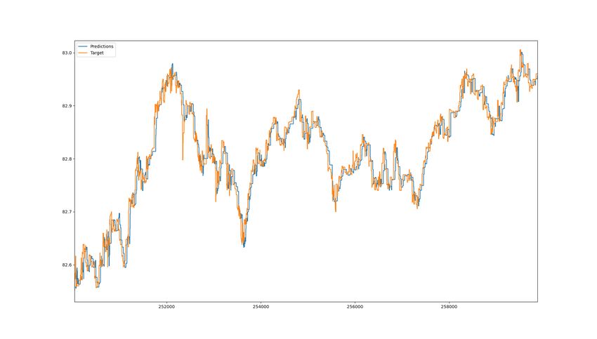
5.2 Two graphs for Swedbank stock price prediction using model
70_100e_lr0.0001_S. Left graph shows prediction for 3 hour window
of Swedbank stock. The left shows a 30min window. Larger figures
can be found in Appendix I. . . . . . . . . . . . . . . . . . . . . . . . 33
5.3 Two graphs for price prediction using model 200_50e_lr0.0001_S.
Left graph shows prediction for 3 hour window of Swedbank stock.
The left shows a 30min window. Larger figures can be found in Ap-
pendix I. . . . . . . . . . . . . . . . . . . . . . . . . . . . . . . . . . . 34
5.4 Two graphs for price prediction using model 700_100e_lr0.0001_S.
Left graph shows prediction for 3 hour window of Swedbank stock.
The left shows a 30min window. Larger figures can be found in Ap-
pendix I. . . . . . . . . . . . . . . . . . . . . . . . . . . . . . . . . . . 34
xiiiList of Figures
5.5 Two graphs for price prediction using model 70_100e_lr0.0001_N.
Left graph shows prediction for 3 hour window of Nordea stock. The
left shows a 30min window. Larger figures can be found in Appendix I. 35
5.6 Two graphs for price prediction using model 200_100e_lr0.0001_N.
Left graph shows prediction for 3 hour window of Nordea stock. The
left shows a 30min window. Larger figures can be found in Appendix I. 36
5.7 Two graphs for price prediction using model 700_30e_lr1e-05_N.
Left graph shows prediction for 3 hour window of Nordea stock. The
left shows a 30min window. Larger figures can be found in Appendix I. 36
5.8 Graph showing the difference between Algorithm A and B. . . . . . . 38
5.9 Graph showing the fastest, mean, and slowest time it took to run n
node-boxes in layer 1, with one node-box in layer two. The test is
done over a 5 minute interval and is measured from the time a node
in layer 1 starts its processing, until the node in layer 2 calculates it
prediction from that timestamp. . . . . . . . . . . . . . . . . . . . . . 39
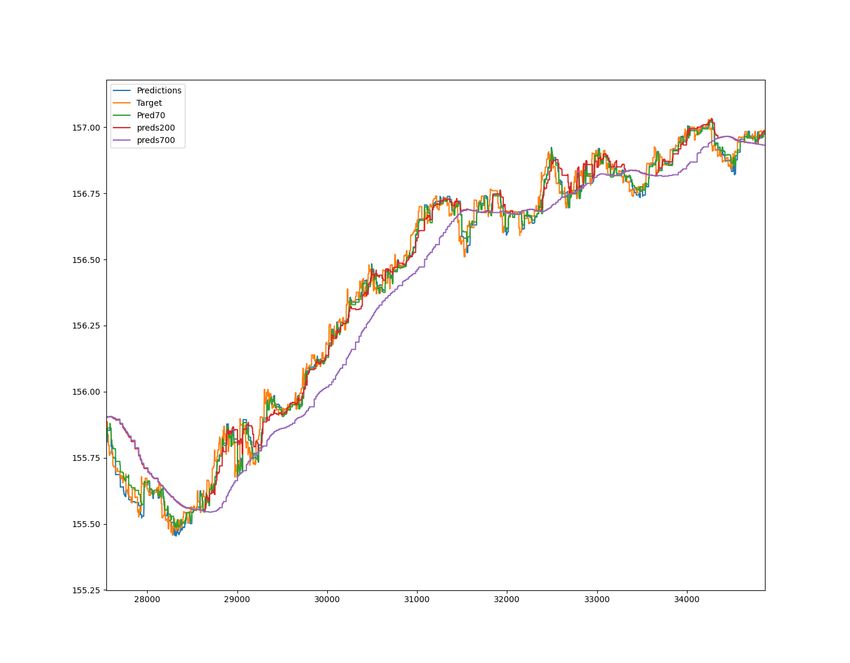
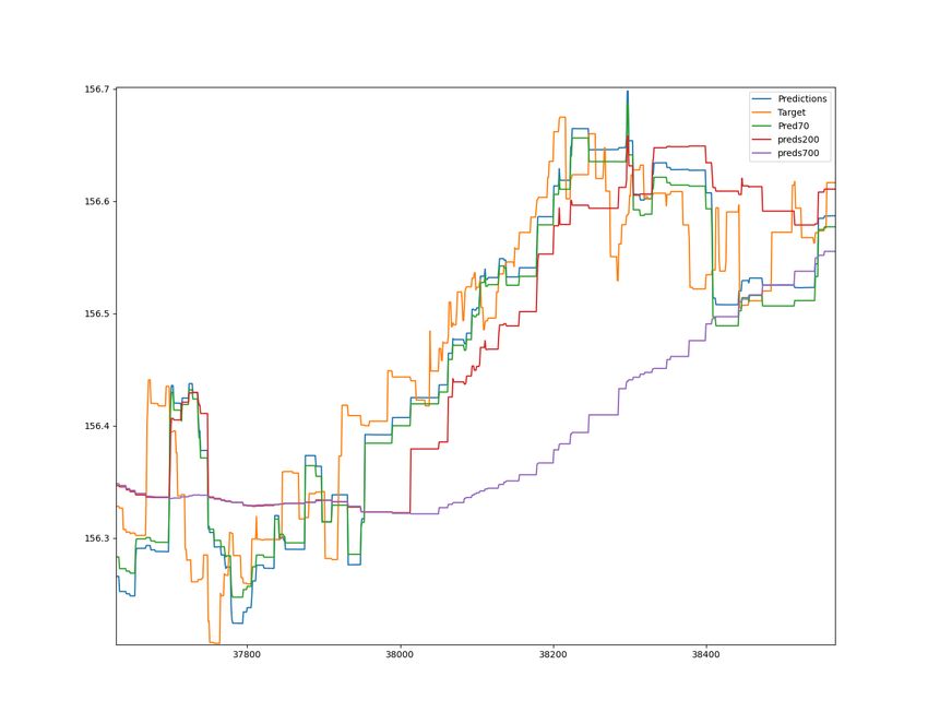
5.10 Graph shows stock price predictions for the distributed model
vol50_lr0.01_None_D. Pred70, Preds200 and Preds700 refers to the
prediction inputs used for the distributed model. Predictions for a 3
hour Swedbank window. . . . . . . . . . . . . . . . . . . . . . . . . . 42
5.11 Graph shows stock price predictions for the distributed model
vol50_lr0.01_None_D. Pred70, Preds200 and Preds700 refers to the
prediction inputs used for the distributed model. Predictions for a 30
min Swedbank window. . . . . . . . . . . . . . . . . . . . . . . . . . . 42
5.12 Graph shows stock price predictions for the distributed model
ema15_macd_rsi5_rsi30_vol100_vol50_lr0.001_NordeaPred70_D.
Pred70, Preds200 and Preds700 refers to the prediction inputs used
for the distributed model. Predictions for a 3 hour Swedbank window. 43
5.13 Graph shows stock price predictions for the distributed model
ema15_macd_rsi5_rsi30_vol100_vol50_lr0.001_NordeaPred70_D.
Pred70, Preds200 and Preds700 refers to the prediction inputs used
for the distributed model. Predictions for a 30 min Swedbank window. 44
5.14 Price prediction result of a section of the test data for Swedbank_A,
using model ema_70_35E_30s_1e-06_time1. X-axis is num-
bering of datapoints from the start of the test set. Data collected
from 08/25-2020 to 15/3-2021 . . . . . . . . . . . . . . . . . . . . . . 46
5.15 Price prediction result of a section of the test data for Swedbank_A,
using model price_200_5E_15s_1e-06_time1. X-axis is num-
bering of datapoints from the start of the test set. Data collected
from 08/25-2020 to 15/3-2021 . . . . . . . . . . . . . . . . . . . . . . 46
5.16 Average test loss for two independent runs using the same data. Nor-
malization is not applied. . . . . . . . . . . . . . . . . . . . . . . . . . 47
5.17 Average test loss for two independent runs using the same data. Nor-
malization applied. . . . . . . . . . . . . . . . . . . . . . . . . . . . . 47
A.1 Prediction of Nordea stock with 70 market orders as input, using
model 70_100e_lr0.0001_N. The graph is shown over a 3 hour window. II
xivList of Figures
A.2 Prediction of Nordea stock with 70 market orders as input, using
model 70_100e_lr0.0001_N. The graph is shown over a 30 minute
window. . . . . . . . . . . . . . . . . . . . . . . . . . . . . . . . . . . II
A.3 Prediction of Nordea stock with 200 market orders as input, using
model 200_100e_lr0.0001_N. The graph is shown over a 3 hour win-
dow. . . . . . . . . . . . . . . . . . . . . . . . . . . . . . . . . . . . . III
A.4 Prediction of Nordea stock with 200 market orders as input, using
model 200_100e_lr0.0001_N. The graph is shown over a 30 minute
window. . . . . . . . . . . . . . . . . . . . . . . . . . . . . . . . . . . III
A.5 Prediction of Nordea stock with 700 market orders as input, using
model 700_30e_lr1e-05_N. The graph is shown over a 3 hour window. IV
A.6 Prediction of Nordea stock with 700 market orders as input, using
model 700_30e_lr1e-05_N. The graph is shown over a 30 minute
window. . . . . . . . . . . . . . . . . . . . . . . . . . . . . . . . . . . V
A.7 Prediction of Swedbank stock with 70 market orders as input, using
model 70_100e_lr0.0001_S. The graph is shown over a 3 hour window. VI
A.8 Prediction of Swedbank stock with 70 market orders as input, using
model 70_100e_lr0.0001_S. The graph is shown over a 30 minute
window. . . . . . . . . . . . . . . . . . . . . . . . . . . . . . . . . . . VII
A.9 Prediction of Swedbank stock with 200 market orders as input, using
model 200_50e_lr0.0001_S. The graph is shown over a 3 hour window.VIII
A.10 Prediction of Swedbank stock with 200 market orders as input, using
model 200_50e_lr0.0001_S. The graph is shown over a 30 minute
window. . . . . . . . . . . . . . . . . . . . . . . . . . . . . . . . . . . VIII
A.11 Prediction of Swedbank stock with 700 market orders as input, using
model 700_100e_lr0.0001_S. The graph is shown over a 3 hour window. IX
A.12 Prediction of Swedbank stock with 700 market orders as input, using
model 700_100e_lr0.0001_S. The graph is shown over a 30 minute
window. . . . . . . . . . . . . . . . . . . . . . . . . . . . . . . . . . . IX
A.13 Prediction of Swedbank stock using the distributed model
rsi30_lr0.01_None_D. The graph is shown over a 3 hour window. . . X
A.14 Prediction of Swedbank stock using the distributed model
rsi30_lr0.01_None_D. The graph is shown over a 30 minute window. XI
xvList of Figures xvi
List of Tables

4.1   The hardware specification of the test bench. . . . . . . . . . . . . . . 25

5.1   MSE and MAE test-set losses for models using min-max normaliza-
      tion. Swedbank between 1 Mars - 19 April . . . . . . . . . . . . . . .          32
5.2   Table showing loss scores over Swedbank test set, 1 Mars to 19 April
      for three different models. Losses for a 10 minute average strategy
      and the offset strategy is also shown. Swedbank single models (the
      best ones, used in dist ) 70 uses time, 200, 700 does not (Deep 30s all)        33
5.3   Table showing loss scores over Nordea test set, 1 Mars to 19 April for
      three different models. Losses for a 10 minute average strategy and
      the offset strategy is also shown. . . . . . . . . . . . . . . . . . . . .      35
5.4   Comparison between Algorithm A and B with different input-sizes. .              38
5.5   Node-boxes benchmark as n : m, where n is the number of nodes in
      layer 1, and m the number of nodes in layer 2 . . . . . . . . . . . . .         38
5.6   Table shows MSE and MAE losses for layer two models used in the
      distributed network. Sorted by MSE loss. Data is Swedbank stock
      price for 13 April - 19 April . . . . . . . . . . . . . . . . . . . . . . .     41
5.7   Table shows MSE and MAE losses for top performing distributed
      models and single stock models. Data is Swedbank stock price for 13
      April - 19 April . . . . . . . . . . . . . . . . . . . . . . . . . . . . . .    41

                                                                                     xvii
List of Tables xviii
1
                           Introduction

The stock market introduces considerable monetary opportunities for investors with
their ears to the ground. Buying when the market is low and selling when it is
high is a common saying in the stock market community. However, employing this
strategy with good timing and precision is a challenging task. To stand a chance,
investors use various predictive techniques to gain some market insight. However,
with the massive amount of traded stocks each second[47] it can be a daunting task
to forecast this massive market. Traditionally investors have used mathematical
models for different kinds of technical analyses, such as the Black-Scholes model
[24], the Heston model [9] or the Gamma Pricing model [25]. These models are
proficient and are still in use today. Other financial tools often used in conjugation
with pricing models are financial indicators such as the Moving Average Conver-
gence Divergence (MACD), the Relative Strength Index (RSI), and the Stochastic
Oscillator (KDJ). Traditionally an investor needs experience to combine all these
models and indicators into a final quality prediction. Studies show that these tech-
nical analysis techniques can increase profitability when being acted upon compared
to a buy-and-hold strategy [6, 50, 37].

Even though several pricing models have shown promising results, some studies still
debate whether the stock market is predictable [44]. The efficient market hypoth-
esis and random walk hypothesis [26] are two examples of such theories debating
stock market predictability, both of which state that the stock price is not based
on historical value or historical movement but instead based on new information.
Moreover, the hypothesis state that the value of a stock is precisely its price and
is determined instantly based on new information. An opposite school of thought
states that the market is indeed predictable and thus is not arbitrarily random. It
states that the market price moves in trends and that market history repeats itself.
Since market price is determined (in the end) by humans selling and buying stocks,
the human psyche determines the market, which does not necessarily react instantly
to new information and is prone to follow trends.
In the hopes of detecting such price trends, several researchers have deployed price
prediction models using neural networks [11, 29]. Neural networks are function
approximators that can learn advanced patterns in data. Furthermore, neural net-
works are universal, meaning they can make predictions on any data, thus not
limiting choices of input data. For example, Chong et al.[5] created a deep neural
network that inputs several 5min intervals of stock return data from several differ-
ent stocks, showing the potential of cross-stock data. Qian and Rasheed [36], using
daily return data, increased their prediction accuracy with an ensemble of several

                                                                                    1
1. Introduction machine learning models, combining artificial neural networks, decision trees, and k-nearest neighbors. This ensemble outperformed all individual models. In the stock market, there are two main types of transactions; market orders and limit orders. Market orders are placed at the current market price and executed nearly instantly. The buyer or seller can not decide the price of the transaction. Setting an asking price lower or higher than the market price creates a limit order, which executes when it matches someone else’s market order. Several researchers have created models which aim to forecast stock market price based on limit order status [45, 41], and other researchers have created models using fixed interval price data, for example, daily price or 5min interval price segments. However, to the best of our knowledge, no research exists describing the use of market orders directly in real-time. 1.1 Aim of The Project The main contribution of this thesis will be to create a model that attempts to forecast the stock market using market orders in real-time. Additionally, the massive quantity of stock information, financial indicators, and earnings reports that can be gathered from the stock market indicate the need for a system that can utilize several such inputs at once. Our goal is to create a system that inputs several different types of predictive information and creates a final prediction. We hypothesize that by utilizing several models, prediction prices from different stocks, and various window sizes, the combined prediction could produce a better result than any single model. Additionally, since we wanted to display the computational power potential of a distributed system, using market orders was a natural decision. 1.2 Risk and Ethical Considerations There are several considerations to have in mind when working with the stock mar- ket. First of all, legalities must be taken into considerations, such as Pump and Dump Schemes[39] and Insider Trading[38]. In the case of this thesis, there is no trading or social interaction done, so there is no risk of any impact on the stock market. As there is no impact on the stock market, there is no need to consider any legalities. An ethical issue to consider is the idea of machine learning trying to understand human behavior for the possibility of earning money (when someone else will lose it). In this case, the program will try to predict stock prices by learning from its previous history. As it will only look at individual market orders, which can be seen as individual trades between humans, it will solely base its prediction on human behavior. It will try to find patterns such as optimism and pessimism, which could correspond to an upcoming rise or fall in the stock market price. However, this is solely speculation, and the program might find other patterns that a human cannot see or understand. 2
1. Introduction

1.3     Limitations
As no historic market order data was found for Stockholmsbörsen, the data was
collected daily as soon as the thesis was proposed. The short time resulted in a
limited amount of historic market order data, which could impact the performance
of the machine learning algorithms.

Our data will consist of market orders, on which we will perform our forecasting.
However, on the stock market, one can perform several different orders. Limit or-
ders are one of those. Limit orders can contain a lot of predictability information,
as shown by Zheng[53]. However, we will not use this data and limit ourselves to
market orders.

The system will use historical stock data, as previously mentioned. Thus, the system
will not use live stock market data. Using live data would have been an intriguing
step to take, but it would add little value to the academic goal of this thesis.

The testing of the distributed part of the thesis was done on a single computer,
as there was not possible to access an extensive network of computers. It would
theoretically work over several computers, but it will not be possible to get any
performance statistics from this thesis.

1.4     Thesis outline
Six chapters divide the thesis. After the introduction, the theory chapter explains
different machine learning aspects and financial indicators.

In chapter 3, we examine previous work of stock prediction with machine learning
and distributed machine learning. Several different techniques that inspired this
thesis are mention.

Chapter 4 explains the machine learning components used in our predictive models
and presents the distributed system.

Chapter 5 describes the result of the thesis and discusses those results. The main
focus of the results is the performance of the predictions, but it also includes some
benchmarks of the distributed system.

Chapter 6 is the final chapter which contains the conclusion and future work.

                                                                                   3
1. Introduction 4
2
                                 Theory

In this chapter, we present relevant background information and theories. The first
sections describe the stock market and relevant financial indicators. Following this,
machine learning information is explained, such as neural networks, backpropaga-
tion, and normalization.

2.1     Stock market momentum
Stock market momentum can be a good indicator for deciding between a long or
short position for any investor. Momentum in the stock market serves to measure
the overall trend based on historical data. Several researchers have shown that
following a strategy based on stock market momentum can be highly profitable [12,
17]. Many indicators can measure stock market momentum, such as RSI or MACD,
which are described in further detail below.

2.2     Lagging and leading indicators
A lagging indicator is an indicator that aims to explain the past. In doing so, one
might find specific trends that indicate what will happen in the future. For example,
if the unemployment rate went up last month and this month, one could say that it
seemingly will rise again next month. This prediction is, of course, not certain, as
the unemployment rate can not climb indefinitely.
A leading indicator on the other hand, says what will happen in the future. Events
that have happened but have not yet affected the process at hand are the basis for
these indicators. For example, if customer satisfaction is way down, the company
performance might not be affected yet, but it might be in the future.

2.2.1    Exponentially weighted moving average
Exponentially weighted moving average (EMA) is a technique used to calculate the
average of rolling data. What makes EMA unique is that it uses the constant α
to determine how much impact older data should have on the new average. The
expression used for EMA is as follows:

                              x̂k = αx̂k−1 + (1 − α)xk

                                                                                   5
2. Theory
where 0 < α < 1. x̂k is the calculated EMA, α is the constant to determine the
importance of older data, also known as the filter constant. x̂k−1 is the most recent
EMA, and xk is the current value [43].
2.2.2 Relative Strength Index
Relative Strength Index (RSI) is a financial indicator that shows the momentum of
a stock. It is an oscillator that ranges from 0 to 100. It is calculated by comparing
the decrease and increase of closing prices over a certain period. Presented by Welles
wilder Jr in 1978, this indicator has seen significant use among investors. Tradition-
ally, an RSI value under 30 is considered a buy signal, and a value over 70 a sell
signal. On average, the RSI value is 50, meaning any RSI over this value indicates a
possibly overbought security, and anything under a possibly oversold security [42].
When calculating the RSI value, a time window first needs to be determined. Welles
Wilder presented a period of 14 periods as an appropriate window. The periods
could be any time intervals, for example, days, weeks, or months. Then two expo-
nentially moving averages are calculated. One over any periods where the closing
price is down, and one for periods with a higher closing price. The RS value can be
determined by:
EM AU P
RS =
EM ADOW N
The following formula is used to convert this relative strength value into a value
between 0 and 100, :
100
RSI = 100 −
1 + RS
The result RSI is the relative strength index value.
2.2.3 Moving Average Convergence Divergence
Moving Average Convergence Divergence (MACD) is a momentum-based indicator
that shows the relationship between long and short-term exponentially moving aver-
ages. In other terms, it helps decide if the market is overbought or oversold compared
to the expected trend, the long-term exponentially moving average. MACD value is
calculated simply by subtracting a short-running EMA by a long-term EMA; thus,
a negative value indicates that the security is underperforming short term, and vice
versa for a positive MACD value [52].
Normally the MACD value is based on a 12 period EMA and a 26 period EMA and
can thus be calculated by the following formula:
M ACD = EM A12 − EM A26
Any MACD movement that crosses zero typically indicates a buy or sell signal.
62. Theory
2.2.4 Volatility
Volatility is a statistical measure of the dispersion of a stock. Dispersion is the
expected range for which a value is predicted to fall within, in other terms, the
uncertainty of a particular position. The uncertainty could be determined by, for
example, the returns or risk of a portfolio.
If the price of a stock falls and climbs rapidly over a certain period, the security can
be considered volatile. How much the price oscillates around the mean price in a time
segment can be interpreted as the volatility value. Thus stocks with high volatility
have less predictability and are considered higher risk than stocks with low volatility.
The variance of the price over some time defines historical volatility. The standard
deviation can measure historical volatility during this period [10].
2.2.5 Price Channels
Price channels are indicators for the highest and lowest price trends over a time
segment. Donchian channels are a way to calculate price channels over different
time segments. The highest point, not including the current timestamp, of the
stock price during a time segment calculates the top channel. During the same time
segment, the stock’s minimum price calculates the bottom channel. The current
price is not included in the time segment to make it possible to see if the current
price breaks the current trend of the top or bottom channel. Breaking the current
trend could indicate a future bear or bull trend [7, 4].
2.3 Machine Learning
Machine learning is a process in which a computer improves a model’s predictability
power by finding patterns in data. By processing a large amount of sample data
points from some distribution, the computer can learn how to interpret the data
and output an accurate result. These inputs could be pre-collected annotated data
or data gathered live via interaction with an environment. Machine learning can
solve many different problems, including item classification, regression, and text
processing. Different machine learning algorithms are thus more suited to specific
problems than others. For example, a decision tree will not be as suited for image
classification as a Convolutional neural network (CNN) [28].
2.3.1 Neural networks
Neural networks are a type of machine learning built by layers of weights and biases
that can learn most classification or regression tasks. Often portrayed as a network of
nodes, a neural network can train to approximate any non-linear function. Between
nodes, an activation function is used that introduces non-linearity to the model,
explained in further detail below. Typically a neural network has several layers,
starting with the input layer. This layer inputs some vector x, which then propagates
72. Theory
forward through the network, finally reaching the output layer. Layers between the
input and output layers are called hidden layers. The term deep neural networks
refer to networks with multiple hidden layers. Neural networks require a larger
amount of data than other machine learning approaches since they contain more
parameters to optimize than other machine learning techniques.
2.3.2 Loss function
Loss functions, or cost functions, present a way to evaluate the performance of clas-
sifiers. It does so by representing the error of some predictions compared to the
target with an actual number. Intuitively this is needed since simply measuring a
classifier in simple wrong, or correct terms does not provide any numerical scale re-
garding how accurate the classifier is. For example, if a model can classify the animal
species of a picture, such as a cat, predicting a dog is better than predicting a whale.
As predictions improve, the value given by the loss function decreases; thus, training
a classifier is an optimization problem where we seek the function f , which maps
inputs to outputs that minimize the loss. Let L(·, ·), be the loss function and
L(f (xi ), yi ) be the loss for prediction f (xi ), where xi is the input vector, and for yi
the target value. For N training samples the optimization problem is [48]
N
1 X
min L(f (xi ), yi )
f N
i=1
Choosing a loss function is an integral part of solving this optimization problem
satisfactorily. For example, a typical loss function for classification tasks is the
cross-entropy loss. The cross-entropy loss is defined as:
L(f (xi ), yi ) = yi log(σf (xi ))
where σ(·) is the probability estimate, and yi is the target label for data point i.
The greater probability value from σ for a correct answer will yield a lower loss.
For regression tasks, a typical loss function is the Mean Squared Error (MSE), also
known as L2 loss. Pn
(yi − f (xi ))2
M SE = i=1
n
where yi is the target value for data sample i and f (xi ) is the predicted value [20].
An alternative way to calculate loss is to use the mean absolute error (MAE), cal-
culated as following:
Pn
i=1 |f (xi ) − yi |
M AE =
n
82. Theory
where f (xi ) is the prediction, yi is the target value for data sample i, and n is the
number of values [49].
2.3.2.1 Backpropagation
Backpropagation is a method for training and fitting neural networks. The word
back refers to the method used in doing this, where gradients are calculated from end
to start, backward, in order to calculate them efficiently. Gradients are the direction
that a function is increasing. Thus, by calculating all gradients for all weights with
respect to a loss function, one can use the gradients with an optimization algorithm,
such as Stochastic gradient descent.
Calculating gradients using more traditional approaches is done by calculating the
gradient for each weight independently, which grows exponentially in a neural net-
work. On the other hand, backpropagation utilizes previously calculated gradients,
finding all gradients in linear time.
If J measures the error between an output from the model and the target, then ∆J
is the movement of the loss function, which we are trying to minimize. We call
∆J the gradient for the loss function that builds up a vector containing all partial
derivatives of weights and biases.
Let, x: the input vector
y: the target vector
J: the loss or error function
L: amount of layers in neural network
W l : the weights connecting layers l − 1 and l
bl : the bias for layer l
f l : activation function for layer l
A single layer in the neural network has the following structure:
z l = W l ∗ al−1 + bl
al = f l (z l )
where al is the output of layer l and al−1 is the previous layers output.
The gradients as mentioned before is calculated from end to start, thus using the
chain rule:
δJ l δal δJ
δW l
= δW
δz l δz l δal
This can be expanded to each layer of the network since:
δJ l l δJ
δal−1
= δaδzl−1 δa
δz l δal
Thus reusing some of the derivatives of layer l for finding the derivatives for layer
l − 1. This propagates through the nodes until the start is reached in which case
a0 = x.
92. Theory
Using all the partial derivatives for the weights and biases, the gradient ∆J is then:
δJ
1
δW
δJ
δb 1
∆J = ...
δJ
δW L
δJ
δbL
2.3.3 Activation functions
Activation functions that output small values for small value inputs and large out-
puts for large value inputs if that value reaches a threshold. This "non-linearity,"
where the output drastically changes at some threshold, introduces neural networks’
ability to learn complex tasks.
2.3.3.1 ReLU
ReLU (rectified linear activation function) has the following property:
x
i, if xi ≥ 0
yi = (2.1)
0, if xi < 0
This property means that y should equal x unless it is lower than 0, and in that
case, it is 0. ReLU is classified as a non-saturated activation function [51].
2.3.3.2 Leaky ReLU
Leaky ReLU is a variant of ReLU which will not set the negative values to 0. The
definition is as following:
x
i, if xi ≥ 0
y i = xi (2.2)
ai
, if xi < 0
where ai is a constant in Z+ [51]. A problem with a regular ReLU is called the dying
ReLU, which results in neurons becoming inactive, making all input result in an
output of 0 [22]. Leaky ReLU solves this problem as it never changes any output to
0 [23]. Research suggests that leaky ReLU gives a better result than regular ReLU
[51].
2.4 Normalization
The purpose of normalization is to bring different data sets to a similar scale. The
reason is to equalize the impact of data points for the machine learning algorithm.
For example, without normalization, data sets with huge numbers could overpower
data sets with smaller numbers, even though both of their data could be equally
important for the machine learning [32].
102. Theory
2.4.1 Min-max Normalization
Min-max normalization is a normalization technique where all values in a data-set
are linearly transformed into fitting between a minimum and maximum value, such
as 1 and 0. Thus, 0 Would correspond to the lowest value in the original data-set
and 1 to the highest value. The function to calculate min-max normalization of a
data point is as follows:
x − xmin
f (x) =
xmax − xmin
where xmin is the original minimum value in the data set and xmax is the maximum
value [32].
2.4.2 Z-Score Normalization
Z-Score normalization normalizes the data in a way that compensates for outliers. If
a single value in a data-set is much higher or lower than the rest of the data points,
using min-max normalization would skew the result, as almost all data points will be
in the lower or higher section of the normalized data. Z-Score normalization solves
this problem by using the mean and standard deviation. The created normalized
data will hover around zero, depending on their standard deviation. The function
for Z-Score normalization is as following:
x−µ
f (x) =
σ
where µ is the mean value of the data set, and σ is the standard deviation [32].
112. Theory 12
3
                         Previous work

Several researchers have published studies applying neural networks to forecast the
stock market. Many have also done so together with financial indicators. This sec-
tion presents relevant work to this thesis and how our approach differs from related
work.

In the scope of input data for stock forecasting, most researches lean towards longer
time segments, often using daily price increments [33, 18, 31]. Using daily prices
provides a broader, more macroeconomic viewpoint for models to make predictions
and requires an extended data collection period. Other research has used shorter
time segments, in the order of minutes, [5, 40], in turn shortening data collection
time. However, we have not found any research which attempts to utilize direct
market orders, which show price jumps in real-time.

Numerous studies are published showing the use of machine learning for financial
forecasting. Furthermore, the use of neural networks for this task has seen much
research [5, 19]. For example, Yang et al. [3] and shows that the daily closing price
of the Shanghai market can be predictable using artificial neural networks. Chong
et al.[5] presents a deep neural network that utilizes historical returns from several
stocks, showing with a sensitivity matrix that stock prices are to some degree cor-
related with each other. Hoseinzade et al. [16] also show that cross stock prices are
correlated using a convolutional neural network (CNN), including time as an input
dimension.

Patel et al. [34] create several machine learning networks for predicting stock market
prices. They investigate the performance of combing different networks in a hybrid
system. Using data from two different Indian indexes, they create an input vector
containing ten financial indicators, such as RSI, MACD, and daily close. From their
experimental results, the use of a two-stage fusion network reigns supreme. The
first stage in the model consisting of a Support vector regression (SVR) following
by a neural network. Patel et al. further explore using different machine-learning
techniques but do not investigate how different indicators affect the result.

Agrawal et al. [1] further investigates the use of financial indicators for stock price
prediction. Training an LSTM network using both volume and price indicators, they
achieve high classification scores. Their experiments reveal that moving average and
MACD correlate highly with the closing price. Dixon et al. [8] designs a deep neural
network which input features consist of lagged price differences and moving averages

                                                                                    13
3. Previous work with varying window sizes. He concludes that DNN is a promising platform for stock price prediction combined with financial indicators. As data size and data complexity increase, predictive models will too. Increasing lo- cal computational power has a limit, financial or physical. Distributed models serve as a solution to this problem, using the power from several computers in parallel. In 2014 Mu Li et al.[21] showed, using a parameter server, they could efficiently distribute a single model’s parameters over several computation nodes. All nodes calculate gradients for different data samples in this system, where-after a server calculated new weights from all gradients, which are returned to the nodes. In [14] Hajewski and Oliveira create an SmSVM distributed network for ensemble learning. Here several worker nodes create predictions that a single master node collects, and the final output is simply the majority vote of all worker predictions. Predictions are used as votes since all models need to approximate the same func- tion; that is, the models try to predict the same target. Ahmed et al. [2] creates a similar network of machine learning models, creating a multi-model ensemble of machine learning models in order to forecast weather conditions. 14
4
                                Methods

This chapter explains the procedure that was applied to obtain our results. Fur-
thermore, it describes utilized tools, libraries, and algorithms.

4.1       Data
All data used in this thesis is based on market orders from Nasdaq OMX Nordiq[30].
The data was gathered using their Download CSV options on the various stock
overviews. Via this button, all daily market orders for each stock could be collected.
Each market order contained price, time of trade, stock id, amount of shares etc.
A script was written which collected this data daily, starting on the 25:th of Au-
gust 2020 and continuing until the 19:th of April 2021. A CSV file for each stock
combined the market orders, making it easy to process several months’ worth of data.

4.1.1     Building features
The raw market orders obtained from the stock exchange need to be processed into
features to be used with machine learning. This section describes what the input
features for the neural networks contain and how the features are created.

4.1.1.1   Price
For each second during trading hours, all new market orders are placed into a fixed
size queue. The size of this queue is referred to as window size for the prediction
models. The values in this queue are appended to a CSV file, where each row cor-
responds to each second. This means that the CSV file contains the window size
amount of market order prices for each second of open hours.

The window sizes tested are 70, 200, and 700. It should be noted that it is impossible
to determine any time segment from the market orders, as it is unknown if the values
in the queue would be replaced in one second or over several minutes.

4.1.1.2   Time
In the CSV file created, each row represents one second. A separate column for each
price can be added to keep track of the time for each market order. The time is

                                                                                   15
4. Methods
normalized for each day. The formula for the normalization is the following:
x
F (x) =
32400
where x is the timestamp adjusted to start at 0 and end at 32400. In other words
the first timestamp of the day gets offset to become zero, the second timestamp one,
and so on until the final timestamp of the day, which will become 32400.
4.1.1.3 Financial indicators
Several financial indicators were calculated in order to be used in neural networks.
The financial indicators used were RSI, MACD, Volatility, EMA, and Price Chan-
nels. These indicators were calculated using the market orders described above.
Many of these indicators describe change over a specific time interval, in which case
several different time variations was calculated, for example, a 10-minute EMA and
a 30-minute EMA.
Donchian channels inspired the implementation of the price channels, but the cal-
culation of the max and min points differ. In order to find a max point for the price
channels, two steps are performed. First, the time segment looked at is split into n
number of sections. Secondly, the maximum points in the first and last section are
selected, which is then used to calculate a straight line between the points in the
following way:
y1 = maxP oint1
y2 = maxP oint2
x1 = timestampM axP oint1
x2 = timestampM axP oint2
∆y y2 − y1
k= =
∆x x2 − x1
m = y − kx = y1 − kx1
After this, we can use the straight-line equation to calculate the y value of the line
between the maximum points at the latest timestamp:
y = kx + m
where x is the current price at the latest timestamp.
4.1.2 Matching x and y data
As the input vector for the machine learning model cannot vary in size, there occurs
a problem during the beginning of the day as the window might not be filled the
first second upon market opening from a lack of market orders. The implemented
solution is to wait until the window has been filled, then begin creating and saving
features. In order to find the matching target value for each input vector, the latest
164. Methods
price is offset with the prediction time. When there is a new day, the window is
cleared, and a new offset is created at that timestamp.
Another issue arises when trying to predict the future in the last n seconds of a day,
where n is the number of seconds predicted into the future. As the last n seconds
will not have any future prediction because the stock market has closed, the solu-
tion is to not predict during these seconds. However, by not predicting the last n
seconds, it also means that the y data corresponding to the last n seconds of a day
is not added to the data set.
4.1.3 Graphs
Plotting the stock price there are periodic straight lines in the y direction. The
reason for this is when a weekend or end of the day occurs, and the price changes
drastically during this time. This also means that the x-axis in the graphs only
shows time when the stock market is open. Therefore the numbers on the x-axis
should be seen as seconds of open stock-market time.
4.2 Distributed system
The distributed system is a system of nodes connected in any desired configuration.
The nodes work together in layers, where each layer sends its output to the layer
below it. For example, in the top layer, the nodes could get their data from a third-
party source, such as a stock exchange. The nodes in the bottom layer output the
final result of calculations in the system. The distributed system code was written
in python to get a prototype up and running as fast as possible.
4.2.1 Node-Box
A Node-Box is the base piece of each node, as seen in Figure 4.1. This Node-Box
contains a processor, inputs, and an output. For example, the processor could be
an algorithm to calculate a financial indicator such as RSI or a machine learning
algorithm. Each Node-Box belongs to a layer, where layer one is the top layer, and
layer n is the bottom layer. The output of one or several Node-Boxes could be a
single or several other Node-Boxes inputs in the layer below. Combining several
Node-Boxes creates the possibility of setups that support redundancy, parallelisms,
and increased computational speed. Figure 4.2 shows a simple example of a single
Node-Box. In this figure, the inputs are the latest 200 market orders for the stock
Swedbank.
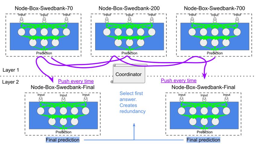
Figure 4.3 shows a connected example of Node-Boxes. In this figure, there are a
total of four nodes, three in layer one and one in layer two. All nodes in layer one
174. Methods Figure 4.1: The base of a Node-Box Figure 4.2: Node-Box with Swebank’s 200 latest market orders send their predictions as an input to Node-Box-Swedbank-Final, which calculates the final prediction with the help of all predictions from layer one. 4.2.2 Smart-sync A data structure has been created to synchronize the different inputs received in a node-box, referred to as asmart-sync structure. The smart-sync synchronizes the data at different timestamps in an asynchronous way, making it fault-tolerant against delays. As the predictions made by machine learning in the processing layers are between 5 and 60 seconds, it is more important that a prediction gets processed as fast as possible and less important that every prediction gets processed. For every second a prediction is not processed, it loses importance, and if more time has passed than 18
4. Methods

Figure 4.3: Three nodes in layer 1, with their targets connected to one node in
layer 2

the prediction time, then we already know the actual price, and the prediction is
useless. The smart-sync handles this issue by having a Window-Size (WS), which
decides how many seconds the smart-sync should keep information.

A single matrix, with a height of the WS and a width of the input-size+1, creates
the base for the smart-sync structure. The input-size is the size of the number of
inputs that should be synchronized. Increasing the width by one makes it possible
to fit a field to check how many cycles have been done. A floor division between the
timestamp and WS calculates this field, denoted as TS // WS. Figure 4.4 visualizes
the structure. In the figure, a field denoted TS % WS can be seen. This field is the
index of the matrix, and TS % WS is how the data should be indexed. Thus, TS %
WS is the timestamp modulo window-size and will place the new data in a cyclic
pattern.

Figure 4.4: Basic structure of the smart-sync.

When new data is to be added, three things are needed:
 1. The timestamp
 2. The node-box id
 3. The data

                                                                                 19
4. Methods
The timestamp is used to calculate which row the data should be put in by us-
ing TS % WS. The node-box id is used to select which column the data should be
placed in. The IDs need to be sequential, as to calculate the column position, the
formula (ID % input-size)+1 is used. Increasing the input size by one is used to
ignore the first field where the number of cycles is kept track of. The data is added to
the corresponding row and column, calculated from the timestamp and node-box id.
When data is added to the smart-sync two checks are done:
1. Compare the incoming data with the field of the current cycle. If the cycle
is the same, add the data to the correct column. If the field is lower than
the incoming data, erase all data in the row and add the new data to the
corresponding column. If the field is higher than the incoming data, then do
nothing. These steps will ensure that the new data overwrites the old data
and that the old data never overwrites the new data.
2. Check if the row where the data was added is filled. If a row is filled, data has
been received from all sources at the specific timestamp, which means that it
can be processed. The smart-sync will thereby notify the processor with an
array of the data at that timestamp.
Figure 4.5 shows an example of added data. The two rows in yellow have not been
processed yet as they are still missing some data. To the left, under the column TS,
shows the original timestamp. The upcoming timestamps would start overwriting
the old ones, as shown in Figure 4.6. A darker green marks the overwritten rows
from the old ones.
The second check when data is added to the smart-sync is tested in two different
ways. In the first one, called Algorithm A, the whole row is iterated to check if it
is filled. This iteration has a complexity of O(n). The second way, Algorithm B, is
to have an integer that counts how many times an element has been inserted into
a row. Every new cycle, the integer resets. Algorithm B has a time complexity of
O(1), as there is no iteration.
Figure 4.5: Smart-sync with data added. The data in green is completed data
that has been sent to be processed. The data in yellow is still missing data.
204. Methods
Figure 4.6: The dark green color indicates old data that has been overwritten.
4.2.3 Applying Techniques in Layer 1
Redundancy, parallelization, or an increase in processing power, can all be applied
to layer one as well. For example, if an increase of processing power is desired, the
number of Node-Boxes in layer one can be doubled and run in cycles the same way
as layer 2. Figure 4.7 shows an illustration of this.
Figure 4.7: Nodes in layer 1 taking turns to calculate their target, possibly achiev-
ing higher processing power
4.2.4 Coordinator
The Coordinator is used to decide the communication between the different Nodes.
The different nodes ask the Coordinator where they should send or receive their pre-
dictions, as seen in Figure 4.8. Depending on how the Coordinator is programmed,
the nodes can be utilized in different ways. Some of the possible utilization could
be for redundancy, parallelization, or an increase in processing power.
4.2.5 Coordinator Protocol
The protocol can be divided into three steps:
214. Methods
Figure 4.8: Node-Boxes asking the coordinator who and how to communicate
1. Discovery
2. Designation
3. Initiation
Discovery
In the Discovery phase, every node-box that wants to join the system connects to the
coordinator and sends its layer position. The coordinator keeps track of the different
node-boxes by saving the IP and port they used to connect. The coordinator can
complete the Discovery phase in two different ways, depending on its configuration.
The first way is to wait until a certain number of node-boxes has connected, and the
second one is to have a waiting time and accept any number of node-boxes during
that time.
Designation
In the Designation phase, the coordinator takes the different node-boxes discovered
in the Discovery phase and assigns a connection between them. This connection
is based on the configuration of the node-box, such as Redundancy, Parallelization,
or increased processing power. When the coordinator has decided which node-boxes
should communicate with which, it returns a key-value store with the following
structure:
’port’: int,
’id’: int,
’server_ip_port’: list(tuple)
port is the port number the node-box should use when hosting a server for its out-
put. id is the unique id of the node-box, which can be used for identification.
server_ip_port is a list of tuples, where each tuple contains an IP address and a
port. The tuples are the node-boxes that the current node-box should listen to and
use as input.
224. Methods
Initiation Lastly the initiation phase begins. In this step, the individual node-
boxes has received their unique key-value store from the coordinator. As soon as
this is received, the node-boxes will start their local server and try to connect to
other servers in the server_ip_port key. As soon as all the node-boxes have con-
nected and started their servers, the system is up and running.
4.2.6 Redundancy
Redundancy can be achieved by having two or more nodes in any layer with the
same prediction model and the same input data. Any prediction of these nodes can
then be used as the final answer. So, for example, if one of the nodes crashes, the
other can continue to operate as usual. Figure 4.9 shows an example of this, where
two Node-Boxes in layer two create redundancy.
Figure 4.9: Two Node-Boxes are doing the same calculations to achieve redun-
dancy.
4.2.7 Parallelization
It is possible to parallelize two different Node-Boxes by sending the same input to
two or more Node-Boxes in any layer. The Node-Boxes will work independently
on their data, and their predictions can be used as desired. Figure 4.10 shows an
example of this with two Node-Boxes.
4.2.8 Cycling node-boxes
If the case would exist where a Node-Box cannot keep up with inference every
second, it is possible to distribute this load over several Node-Boxes, which would
increase the processing power. Every Node-Box would receive features to predict
every n seconds, where the first Node-Box gets it on second n, the second one on
234. Methods Figure 4.10: Two Node-Boxes doing different calculations to parallel processing. second n + 1, and so on. When every node has received features to predict, it will restart again with node n. An example can be seen in Figure 4.11. Figure 4.11: Two nodes cycling their workloads, increasing the processing power 4.2.9 Financial Indicator Node The Financial Indicator Node (FI-Node) is a node that only calculates different Financial Indicators, such as MACD or RSI. The purpose is to add more features to any Node-Box in an effort to improve the machine learning performance. The FI-Node calculates financial indicators for any single stock, such as Swedbank, but could also calculate financial indicators for an index if desired. Figure 4.12 shows an illustration of this. 24
4. Methods

Figure 4.12: FI-Node, which gives financial indicators as features to the Node-Box
in layer 2

4.2.10     Test Bench
When running any benchmarks or tests is was run on the system shown in Table
4.1.

 CPU     Intel i5-4670k (4 cores), Overclocked to 4,3 GHZ
 GPU     Nvidia GTX 970
 RAM     32 GB DDR3
 OS      Pop!_OS 20.10 (based upon Ubuntu 20.10)

Table 4.1: The hardware specification of the test bench.

4.3      Stock predictor
This section describes the machine learning libraries, input feature construction,
and network architecture used in this thesis. It further describes how the training
for layer one models and created and describes the combined distributed system.

4.3.1     PyTorch
The machine learning library, PyTorch, creates and trains models. PyTorch is an
open-source library that Facebook mainly develops. This thesis uses the python
interface but is executed in a C++ environment. PyTorch introduces a tensor data
structure, a matrix-style structure developed for fast computations on graphic pro-
cessing units (GPU). It also contains an auto differentiation feature, which alleviates
training neural networks through backpropagation[35].

                                                                                    25
You can also read