Real-to-Sim Registration of Deformable Soft Tissue with Position-Based
←
→
Page content transcription
If your browser does not render page correctly, please read the page content below
Real-to-Sim Registration of Deformable Soft Tissue with Position-Based
Dynamics for Surgical Robot Autonomy
Fei Liu†,1 Member, IEEE, Zihan Li†,1 , Yunhai Han1 , Jingpei Lu1 , Florian Richter1 Student Member, IEEE
and Michael C. Yip1 Senior Member, IEEE
Abstract— Autonomy in robotic surgery is very challenging
in unstructured environments, especially when interacting with
deformable soft tissues. The main difficulty is to generate
model-based control methods that account for deformation
arXiv:2011.00800v3 [cs.RO] 30 Apr 2021
dynamics during tissue manipulation. Previous works in vision-
based perception can capture the geometric changes within
the scene, however, model-based controllers integrated with
dynamic properties, a more accurate and safe approach, has
not been studied before. Considering the mechanic coupling
between the robot and the environment, it is crucial to develop
a registered, simulated dynamical model. In this work, we
propose an online, continuous, real-to-sim registration method
to bridge 3D visual perception with position-based dynamics
(PBD) modeling of tissues. The PBD method is employed to
simulate soft tissue dynamics as well as rigid tool interactions
for model-based control. Meanwhile, a vision-based strategy
is used to generate 3D reconstructed point cloud surfaces
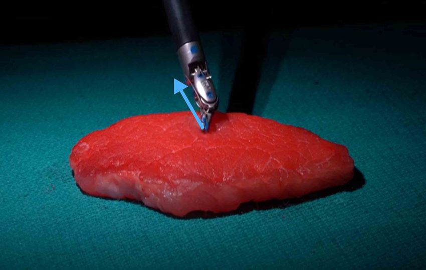
based on real-world manipulation, so as to register and update Fig. 1: A demonstration of real-to-sim registration for deformable
the simulation. To verify this real-to-sim approach, tissue tissue. The top figures show the real images, and the bottom figures
experiments have been conducted on the da Vinci Research show the corresponding registered meshes before (left) and after
Kit. Our real-to-sim approach successfully reduces registration (right) manipulation using our method. The blue arrow indicates
error online, which is especially important for safety during the grasping direction.
autonomous control. Moreover, it achieves higher accuracy in
occluded areas than fusion-based reconstruction.
these methods require the complete observation of the de-
formable tissue and are not able to handle the occlusions. A
I. I NTRODUCTION
Finite Element Method (FEM) implemented with the SOFA
Surgical robotic autonomy has drawn significant interest framework [10] was used in [11] during procedures involving
in recent years, as it may help ease surgeon fatique, reduce inserting needles into tissues. However, FEM as a general
human errors, or address lack-of-access to timely, life-saving strategy has a significant problem that one cannot explicitly
surgery in remote or under-served communities [1]. Regard- apply position constraints on the simulation easily, so the
less of what type of surgical task is being performed, which registration between real world and simulation cannot be well
is essential for manipulating tissues safely. defined. Works in autonomous debridement [12] and tissue
Different approaches to 3D reconstruction and tracking tensioning [13], [14] applied learning method to identifying
from cameras have been proposed for dynamic and de- proper tissue properties from visual input. However, none
formable environments, such as structure from motion (SFM) of these works considered the physical dynamics explicitly.
[2], simultaneous localization and mapping (SLAM) [3], They directly extract control policies from vision rather than
[4], and fusion-based model-free tracking [5], [6]. A more establish an underlying model and solve the model-based
comprehensive review can be found in [5]. However, visual control problem, which limits the performance beyond the
information alone is not capable of providing internal dy- training environments.
namical properties of soft tissues, such as mechanics, inertial Another way to integrate tissue dynamics is to build
properties – the features that are needed for accurate model- a physical-based surgical simulator. In computer graphics,
based control. position-based dynamics (PBD) is a popular method of
To address the aforementioned problem, several works simulating object deformation [15] in real-time. It has shown
have been conducted to estimate the partial tissue dynamics great potential in the application for surgical simulation
and deformations by using reinforcement learning [7], defor- scenarios, such as biopsies [16] and cutting [17].
mation Jacobian [8], and adaptive estimator [9]. However, Taking advantage of fast real-time PBD simulation, we
intend to bridge the gap between visual perception and
† Equal contributions. physical tissue dynamics modeling through an online, con-
1 Advanced Robotics and Controls Lab, University of California San
Diego, La Jolla, CA 92093 USA. {f4liu, zil027, y8han, tinuous, real-time registration method. We call this real-to-
jil360, frichter, yip}@ucsd.edu sim registration. The method incorporates the point cloud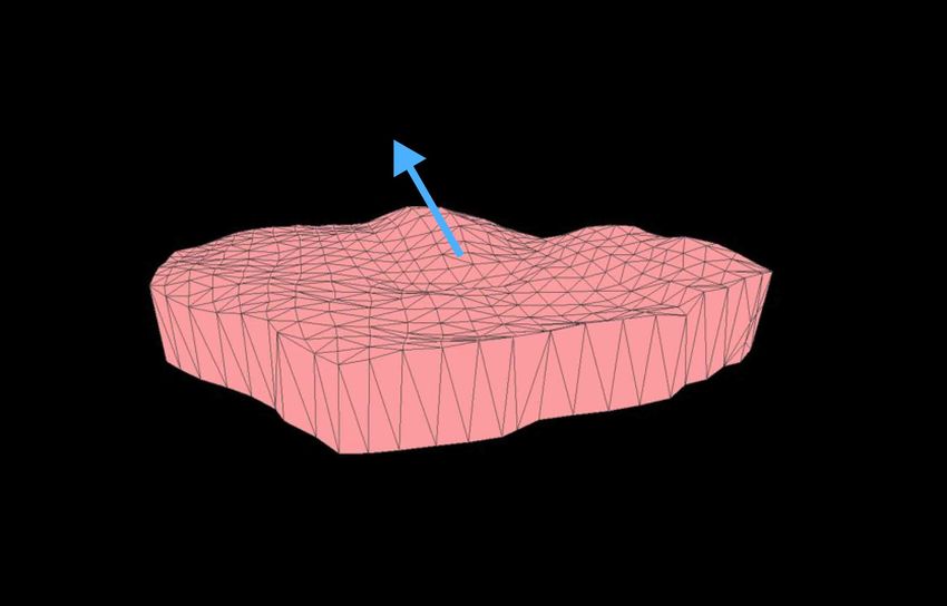
extracted from cameras at each frame to update the simulated         Algorithm 1: Simulation Process
surface particles in PBD. This points-to-particles correspon-    1    x∗ = xt + ∆tζvt + ∆t2 M−1 fext (xt )       . prediction
dence can be viewed as a surface constraint and solved as a      2    while iter < SolverIterations do
registration cost function by gradient descent. To the best of   3       for constraint C ∈ C do
our knowledge, this is the first work to perform deformation                      iter
                                                                 4           [∆x]C = ∇x∗ C                 . constraint solving
registration for simulation using PBD, relying on real-world                  ∗        ∗     iter
                                                                 5           x = x + [∆x]C
observation of tissue deformation (Fig. 1). The contributions
                                                                 6       end
of our method are summarized as,
                                                                 7    end
  1) a position based framework for surgical simulation          8    xt+1 = x∗                              . update position
     involving physical constraints (i.e. distance, volume       9

                                                                      vt+1 = xt+1 − xt /∆t                   . update velocity
     represented by particles, etc.),
  2) a real-to-sim matching algorithm for registration is
     applied as an additional dynamic constraint for PBD,
  3) integration of surgical perception framework (SuPer)        constraint and replace the triangle area preservation with
     proposed in [5], which can potentially improve the          tetrahedron volume preservation.
     accuracy of fusion-based reconstruction in the occluded
     areas.                                                                 Cdistance (x1 , x2 ) = |x1 − x2 | − d0
                                                                                                    1                         (1)
Our method was implemented on a da Vinci Research Kit              Cvolume (x1 , x2 , x3 , x4 ) = (x2,1 × x3,1 ) · x4,1 − v0
[18]. Multiple tissue manipulation experiments were con-                                            6
                                                                    Where, d0 is the initial distance between x1 ∈ R3
ducted to highlight its effectiveness and accuracy. We believe
                                                                 and x2 ∈ R3 and v0 is the initial tetrahedron volume
that this real-to-sim method is a fundamental step towards
                                                                 represented by the four corner particles x1 , x2 , x3 , x4 ∈ R3 .
generalizable surgical automation.
                                                                 The position corrections [∆xi ]distance and [∆xi ]volume can be
                      II. S IMULATION                            obtained respectively.
                                                                    2) Shape Matching: Shape matching is a geometrically
A. Position-based Dynamics (PBD)                                 motivated approach of simulating deformable objects [23] to
   Physical simulation has been studied in the past decades      preserve rigidity. The basic idea is to separate the particles
and can be classified into mesh-based ([10], [19]) and mesh-     into several local cluster regions and then, to find the best
free methods ([20], [21]). For all methods, there is an          transformation that matches the set of particle positions
inherent trade-off between physical accuracy, computational      (within the same cluster) before and after deformation,
stability, and real-time performance. Unlike physical sim-       denoted by {x̂i } and {xi }, respectively.
ulators, the PBD method provides a real-time solver and             The corresponding rotation matrix R and the translational
stable time integration scheme that makes it fast and robust     vector t̂, t of each cluster are determined by minimizing the
to use in practice. Different materials are identified not by    total error,
                                                                                                  n
their physical parameters but through constraint equations                                       X
                                                                                                     kR x̂i − t̂ + t − xi k22

which define particle positions and position-derivatives. This          arg minR∗ ,t̂∗ ,t∗ =                                  (2)
                                                                                               i
representation of positional evolution can naturally build the   where n represents the number of particles in the correspond-
link from visual perception to image data, as it could force     ing cluster. The detailed solutions can be found in [15] by
a topological constraint on the surface particles of a scene.    polar decomposition of the transformation matrix. Thus, the
It also allows us to combine different types of geometrical      position corrections of shape matching can be computed as
constraints (such as distance, volume, etc.). More details of
                                                                         [∆xi ]shape matching = R∗ x̂i − t̂∗ + t∗ − xi

                                                                                                                           (3)
PBD method can be found in [15].
   In our research, the simulated object is defined as a set       The above constraints can be computed through the Gauss-
of N particles and M constraints. Given the current position     Seidel method [15] (Lines 3 to 6 in Algorithm 1).
x and velocity v of the particles, the simulation process is
                                                                                        III. R EGISTRATION
described in Algorithm 1. A force fext acts on each particle,
which only includes gravity in this work. When a local              To ensure our PBD simulator matches the real-world
set of particles is grasped by a manipulator, their positions    observations, we propose a real-to-sim registration algo-
are constrained to the manipulator’s trajectory under the        rithm, which achieves position correction by minimizing
assumption that they are fixed to the end effector.              a registration cost. The main contribution of our work is
                                                                 bridging the gap between the PBD simulation and a 3D visual
B. Geometric Constraints                                         observation. In this work we will leverage the perception
   We include several geometric constraints for simulation of    framework introduced in [5], which is a fusion-based method
the particle dynamics to generate the soft tissue deformation.   for surface reconstruction and deformable tissue tracking.
   1) Distance Constraint & Volume Preservation: In [22],           An outline of our real-to-sim registration is shown in
the authors proposed a 2D PBD-based surgical simula-             Algorithm 2 and visualized in Fig. 2. Signed distance
tion framework. In this work, we adapt the same distance         function (SDF) field is used in this work to evaluate the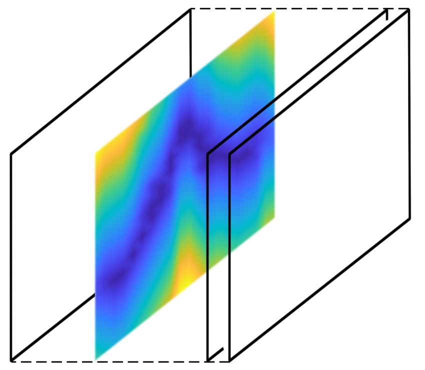
Fig. 2: The real-to-sim registration algorithm flow involves both the observed point cloud and PBD simulation. P 0 and P t are the observed
point clouds at time 0 and t respectively. X 0 and X t are the simulated volume meshes (represented by particles) in PBD. M0 and Mt
are the extracted surface (a subset of volume mesh) particles. Ωt is the inverse deformation field (IDF) of M0 described along a 3D
grid. Φ0 is the initial signed distance field (SDF) of P 0 defined along the grid, and Φt is the approximated SDF. The registration cost
gradient ∇J t can then be calculated for PBD simulation updates. The math symbols can also be referred to Algorithm 2.

    Algorithm 2: Real-to-Sim Registration Flow
     input : Initial point cloud P 0 , registration stiffness
              λregi
1    X 0 ← P0                         . initial PBD particles generation
2    Φ0 ← P 0                                   . initial SDF generation
3    t=0
4    while not terminated do
 5       Mt ← X t                   . extract surface particles from PBD     Fig. 3: The boundary space (left) is discretized into Eulerian space
 6       Ωt ← Mt                    . calculate inverse deformation field    grids. The simulated tissue surface is represented by mesh particles
                                                                             inside it. Each space point p is weighted by its 8 surrounding grid
 7       P t ← {pt1 , pt2 , · · · }            . get current point cloud     cube vertices vi according to the normalized distance to each face.
 8       Φt ← Φ0 , Ωt , P t               . approximate deformed SDF
 9       J t ← Φt , P t                      . calculate registration cost
10       ∇J t ← Mt                      . calculate registration gradient    computed and all other SDF values are estimated by tracing
11       X t ← ∇J t , λregi . perform PBD simulation with registration       back with the IDF Ωt . The SDF values are then evaluated
12       t ← t + ∆t                                                          as registration cost (detailed in Section III-C) and taken into
13   end                                                                     PBD simulation.

                                                                             A. Initial SDF Generation
                                                                                In practice, instead of constructing a continuous 3D SDF
difference between observed point cloud data and simulated                   field, we only discretize the boundary space that envelops
deformation. We firstly define the initial SDF field Φ0 ,                    the whole deforming mass into a 3D Eulerian grid V, as
in a discrete Eulerian 3D space, using the first frame of                    shown in Fig. 3. Only the discrete SDF value at each grid
reconstructed point cloud data P 0 (detailed in Section III-A).              vertex v ∈ R3 is calculated. Then the SDF value of a
The SDF indicates the signed distance between a given space                  position within (but not necessarily falling on) this grid can
point and the initial surface mesh constructed from point                    be identified via linear interpolation of its surrounding eight
cloud M0 . Meanwhile, the PBD simulation is also initialized                 grid cube vertices ({v1 , v2 , v3 , · · · , v8 }) in which the point
using the initial surface mesh. We extend the surface mesh                   resides. The interpolation weights are calculated according
into a volumetric tetrahedron mesh X 0 along the gravity                     to the normalized distance to each face of the surrounding
direction with pre-assumed thickness of the soft tissue. Then                cube, named by {α, β, γ, 1 − α, 1 − β, 1 − γ}. For any given
at each time t, we construct an inverse deformation field                    point in space q ∈ R3 , the SDF vector is interpolated as
(IDF) Ωt by taking the simulated surface mesh Mt as input                      Φ0 (q) = (1 − α)(1 − β)(1 − γ)Φ0 (v1 )
(detailed in Section III-B). Thus, the deformed SDF Φt of                             + (1 − α)(1 − β)γΦ0 (v2 )                              (5)
the point cloud P t can be approximated by tracing back the                                                   0
                                                                                      + (1 − α)β(1 − γ)Φ (v3 ) + ... + αβγΦ (v8 )    0
surface deformation using IDF Ωt ,
                                                                             where Φ0 (vi ), i ∈ {1, 2, · · · , 8} is the initial SDF vector
                Φt (P t ) ≈ Φ0 (P t + Ωt (Mt ))             (4)              for its surrounding grid vertices. This is calculated by the
     To sum up, only the SDF field at initial frame Φ0 is                    distance to corresponding closest point p0∗ ∈ R3 inside the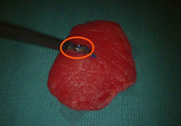
Fig. 4: The demonstration of inverse deformation field (IDF). For
simplicity, we visualize the 3D IDF (left) by one 2D Eulerian
grid slice (middle and right). Middle figure shows the inverse
deformation vectors of current surface particles (red points on solid
curve) regarding initial particles (black points on dashed curve).
Right figure shows the diffusion of whole grid vertices.

received initial point cloud frame P 0 . Then, the initial SDF
                                                                        Fig. 5: The demonstration of reconstructed volume meshes on the
vector for each grid vertex v ∈ V is defined by                         tissue manipulation dataset. The top-left figure shows the real image
                Φ0 (v) = v − p0∗                                        and the top-right figure shows the tracked surface particles using the
                                                            (6)         surgical perception framework. The bottom figures show the sim-
                p0∗ = arg minp0 ∈P 0 kv − p0 k2
                                                                        ulation results, with (left) and without (right) the registration. The
B. Inverse Deformation Field (IDF)                                      estimated mesh is more realistic after the real-to-sim registration.
   An inverse deformation field (IDF) can be computed by
tracing back the positions of particles to their initial ones, as       tration process is performed as a numerical gradient descent
shown in Fig. 4. First, for each surface particle mti ∈ R3 in           via a backwards difference approach,
the surface mesh set Mt at current time t, we can obtain the                                  J t (mt + ∆m) − J t (mt )
deformation vector by subtracting the corresponding particle                         ∇m t J t =                         (10)
                                                                                                          ∆m
at time t = 0, m0i ∈ R3 as,
                                                                        where ∆m ∈ R3 is a manually assigned small forward
                      Ωt (mti ) = m0i − mti                      (7)    deformation of surface particles.
where   mti ,   m0ican be acquired directly from the PBD                D. Constraint Satisfaction for Real-to-Sim Registration
simulation.
                                                                           Traditional point-to-point registration will force all par-
  Then, for all of the discreate Eulerian grid vertices v ∈
                                                                        ticles on the surface to the observed position, which may
V in the initial SDF space, we define their corresponding
                                                                        violate the object’s geometrical structure if the tracking al-
deformation field vector as,
                                                                        gorithm provides an incorrect correspondence. To avoid this,
               Ωt (v) = Ωt (mt∗ )
                                                            (8)         we perform correspondence-free corrections by minimizing
               ∗ = arg minm0∗ ∈M0 kv − m0∗ k2                           the difference between two surfaces instead of pairs of cor-
where ∗ is the index of the closest particle to the grid vertex         responding points. Since point-to-point correspondences are
v in initial surface set M0 . It can be viewed as a diffusion           not strictly enforced, the error can hardly be zero. However,
operation for each Eulerian grid vertex. For any other point            by pulling each simulated particle along the total registration
q ∈ R3 in the initial SDF space, the deformation field is               gradient, the points will finally rest in a neighborhood of the
calculated using a similar interpolation method as the one              observation and consist of a similar tissue surface.
shown in Eq. 5.                                                            In Eq. 9 and 10, the summation of registration cost
                                                                        J t and the gradients of each surface particle ∇m J t are
C. Real-to-Sim Registration Cost
                                                                        obtained, which correspond to another constraint C and ∇x C
   In this section, we define the real-to-sim registration cost         in Algorithm 1, respectively. Thus, the position correction
function. This registration refers to the matching between the          introduced by real-to-sim registration can be directly updated
immediate visual perception and the PBD simulation of the               as an additional, soft constraint. We introduce a stiffness
current timestamp. The matching cost can be defined as the              parameter λregi ∈ [0, 1] to tune this constraint:
summation of the deformed SDF values approximated using                             [∆x]registration = λregi · ∇m J t , x = m       (11)
the surface mesh particles Mt and all visual perception data,
                                                                        With the stiffness term λregi , the simulator will not force
i.e. point cloud P t . Suppose pti ∈ R3 is the i-th point in P t ,
                                                                        the surface immediately to the observed point cloud, which
then the registration cost function is formulated as
                          Xn                                            avoids oscillation while trying to satisfy different constraints
              J t (Mt ) =    kΦt (pti )k22 , pti ∈ P t       (9)        in Gauss-Seidel style.
                           i=0
                                                                                      IV. E XPERIMENTS AND R ESULTS
where n is the number of points in the reconstructed point
cloud P t .                                                             A. Experiment Setups and Evaluation Metrics
   Since our algorithm consists of multiple discrete grid                 In order to demonstrate the effectiveness of the proposed
calculations which precludes analytical gradients, the regis-           registration framework, we conducted experiments on two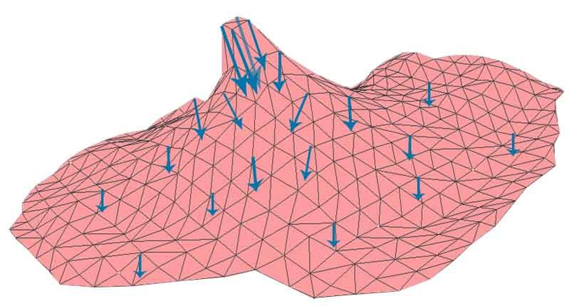
cloud pobs
i ∈ P t and the corresponding simulated surface
particle mi ∈ Mt :
sim
n
X
Errorwith/without regis = msim
i − pobs
i 2
(12)
i
where, n is the total number of simulated surface particles.
It is necessary to mention that the evaluation metric defined
here is different from the registration cost (which is using
SDF) in the previous section, and will be averaged over
Fig. 6: The visualization of the error between the simulation and timestamps or number of particles in the following data
observed surface particles before (left) the after (right) the real-to- analysis. The surface particles are from PBD simulation at
sim registration (averaged in timestamp). After the registration, the
real-to-sim error is reduced significantly around the pinch point. each time t. Both the simulation cost with registration and
the one without are documented.
X-Y Error (W/O Regis.) X-Y Error (W Regis.)
Z Error (W/O Regis.) Z Error (W Regis.) B. Chicken Skin Experiment
0.6
In this experiment, a surgical tool with a gripper was used
to lift the chicken skin, as shown in Fig. 5. If we performed
Error (mm)
PBD without our registration method, the simulated volume
0.4
mesh would not deform to the same shape as visually
observed. The quantitative comparison results shown in Fig.
0.2
6 also support our observation. After performing real-to-
sim registration, PBD simulation was able to capture the
0 surface deformation as observed from point cloud. In the
0 10 20 30 40 50 60 70 80 90
Timestamp left of Fig. 6, the errors around grasping areas is abnormally
high due to lack of realistic tissue parameters in simulation,
Fig. 7: The real-to-sim registration errors (averaged over all surface while in the right figure, our method significantly reduce the
particles) on XY -plane and on Z-direction (gravity direction). The error between simulation and observation. From Fig. 7, we
errors both in the Z-direction and XY -plane are decreased after can tell that our method corrects both the errors in the Z-
registration.
direction (gravity direction) and in XY -plane. However, the
XY errors remain large even after registration. It is caused
different live environments involving soft tissues manipulated by the uncertainties, i.e., noises from stereo reconstruction,
using the da Vinci Research Kit (dVRK [18]): (1) the tracking noises of the surgical tool etc. Meanwhile, the
Chicken Skin Experiment from SuPer dataset [5], and (2) deformation is mostly happening in anti-gravity direction (Z)
the Pork Steak Experiment, which consists of four motion in our grasping experiments, while only small deformation
trajectories: lift, cube, butterfly and sine wave. For each (in millimeter level) is presented in XY -plane. The noise
experiment, the visual perception framework [5] was utilized is relatively large comparing to XY deformation and un-
to track the tissue surface point cloud as the real-world dermines the real result. Hence, we will focus on the error
observation after masking out the background area. The vol- introduced in the Z-direction in the following experiments.
ume meshes (represented by particles) were created from the
initially reconstructed point cloud before the manipulation, C. Pork Steak Experiment
and the PBD simulation process started as the control actions In this experiment, we tested our method by manipulating
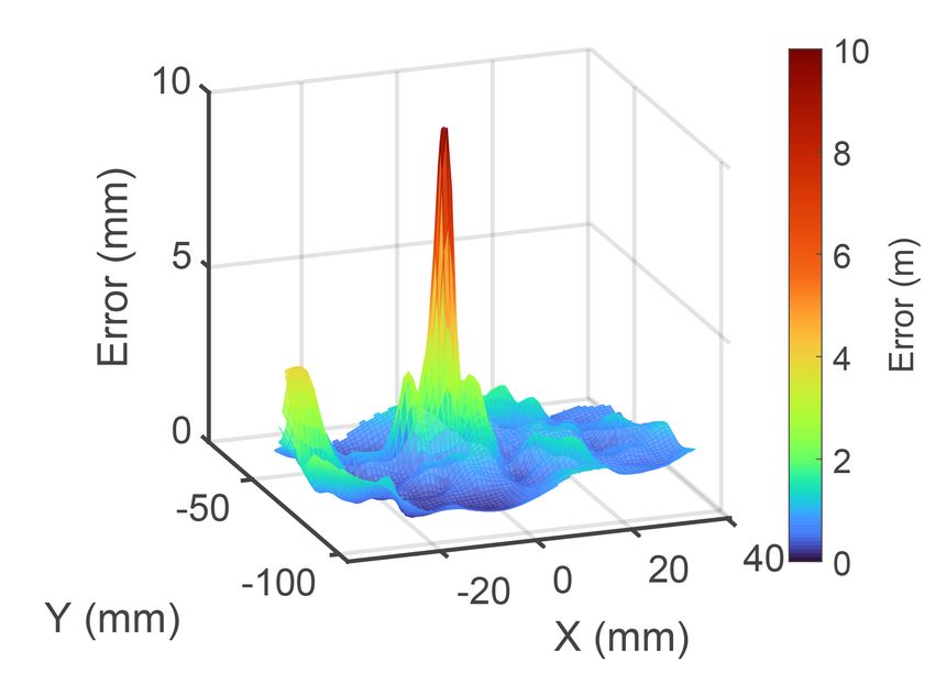
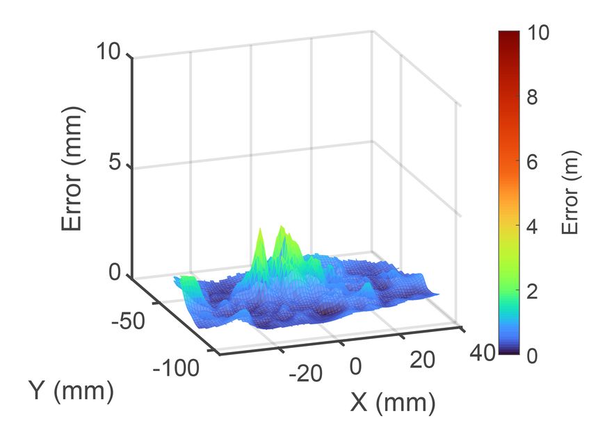
were executed. the tissue with four different moving trajectories, which are
The control actions involved grasping the surface of the shown in the first column of Fig. 8. The following columns
tissue and producing a tissue deformation to track for the show the plots of real-to-sim errors in time (averaged over
real-to-sim method. The grasp location was defined in the all surface particles) and the heatmaps of the real-to-sim
simulation by the four closest surface particles to the end- errors in space (averaged over the timestamps) with and
effector. During the registration, their positions were cor- without registration, repectively. The experiment results show
rected using the shape matching method with the observed the importance of online, real-to-sim registration in properly
point cloud. The simulation boundary conditions were satis- representing the scene deformation.
fied by fixing the boundary particles’ position from the initial The areas circled by the black dash lines in the heatmaps
volume mesh, where the real chicken skin and pork steak are the regions occluded by the surgical tool during the
were fixed on the table. This would be representative of an manipulation (see Fig. 9). This information is typically
internal cavity where tissue would not typically be separated not available, but we were using the SuPer framework [5]
from connected organ before cutting. for reconstruction, which does spatio-temporal fusion under
In order to quantitatively evaluate the system performance, partial occlusions to estimate their position. Because these
we evaluated the registration cost of both whole surface and points are being only estimated and not measured in the
individual surface particles. We define the evaluation metric video frame, we can exclude those occluded points from
as the L2 norm between the 3D position of the observed point our overall error measurements. The second column in Fig.
Error before registration (w/o mask) Error after registration (w/o mask)
Error before registration (with mask) Error after registration (with mask) 10 10
40 2.5 -180 -180
8 8
2 -160 -160
Error (mm)
Error (mm)
Y (mm)
Z (mm)
6
Y (mm)
6
Error (mm)
30
1.5 -140 -140
4 4
-120 -120
20 1
-100 2 -100 2
-30
0.5
-40 -145
-140 -80 0 -80 0
-50 -135
X (mm) 0 -60 -40 -20 0 20 -60 -40 -20 0 20
Y (mm) 0 10 20 30 40 50 60 70 80
X (mm) X (mm)
Timestamp
1.2 8 8
-180 -180
1
30 6 6
-160 -160
Error (mm)
Error (mm)
0.8
Error (mm)
Z (mm)
Y (mm)
Y (mm)
25 -140 4 -140 4
0.6
-120 -120
20 0.4
2 2
-100 -100
-34 0.2
-38
-42 -135 -140
-145 -80 0 -80 0
-125 -130 0
X (mm) Y (mm) 0 10 20 30 40 50 60 70 80 -60 -40 -20 0 20 -60 -40 -20 0 20
Timestamp X (mm) X (mm)
3 6 6
-180 -180
40 2.5
-160 -160
Error (mm)
Error (mm)
4 4
Z (mm)
2
Error (mm)
Y (mm)
Y (mm)
30 -140 -140
1.5
-120 2 -120 2
1
20
-30 -100 -100
-35 0.5
-40 -140 -150
-120 -130 -80 0 -80 0
0
X (mm) Y (mm) 0 20 40 60 80 100 120 -60 -40 -20 0 20 -60 -40 -20 0 20
Timestamp X (mm) X (mm)
1.5 6 6
50 -180 -180
-160 -160
Error (mm)
4
Error (mm)
1 4
Error (mm)
Z (mm)
Y (mm)
Y (mm)
40
-140 -140
30 0.5 -120 2 -120 2
-30 -100 -100
-40 -150
-50 -130 -140 0 -80 -80 0
-120 0
X (mm) 0 50 100 150 -60 -40 -20 0 20 -60 -40 -20 0 20
Y (mm)
Timestamp
X (mm) X (mm)
Fig. 8: The quantitative results of the proposed real-to-sim registration method for four different manipulations (one for each row) in
Pork Steak Experiment. The plots in the first column show the real tool trajectories (lift, cube, butterfly, and sine wave from top to
bottom, respectively). The second column shows the plots of real-to-sim errors before and after registration in time by averaging the
surface particles (with and without masking of the occluded particles). The third and fourth columns show the real-to-sim errors in space
(averaged over the timestamps) with and without registration respectively. The areas circled by dashed lines indicate the regions occluded
by the tool. Our method significantly reduced errors in different manipulation tasks.
V. D ISCUSSION AND C ONCLUSION
In this paper, we have introduced a real-to-sim registration
method to initialize and effectively register a PBD simulation
to a real, live surgical scene. Several real experiments have
been conducted on dVRK with detailed quantitative error
Fig. 9: An example of the inaccurate reconstructions of the regions analysis. Our method provides a crucial link between volu-
occluded by the surgical tool. The left figure is the real scene. The
middle figure is the observed point cloud and the right figure is the metric PBD simulations, which is necessary in model-based
simulation result without registration. The orange circles indicate control, and surface reconstructions of deformable tissue
the occluded regions in each figure. It is obvious that the observation based on camera images.
of the occluded regions is inaccurate. For future works, we will investigate control policies
for surgical automation that use the proposed real-to-sim
8 shows the mean real-to-sim registration errors (with and registration. The proposed geometrical constraints are differ-
without mask) in time. The red solid line shows the error ent from traditional force models using material parameters
with registration averaging over all surface particles, while which may result inaccuracy. More constraints can be ex-
the blue solid line shows the averaged error with registration ploited to increase realistic of simulation. Furthermore, the
after excluding the particles that are occluded for more than registration gradient can be applied to optimizing a control
half of the total frames. Since the SuPer framework deals policy for a specific tissue manipulation task using model
with the occluded area using the history information for predictive control.
fusion, our method provides a more reasonable estimation ACKNOWLEDGEMENT
of the occluded area by using the PBD simulation. This is
Many thanks to Hanpeng Jiang for experimental setup.
another contribution of our work.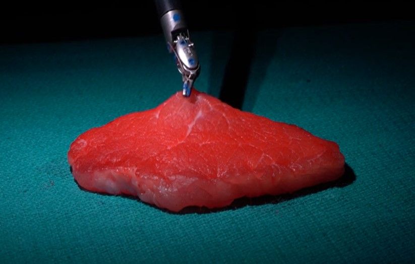
R EFERENCES                                        [18] P. Kazanzides, Z. Chen, A. Deguet, G. S. Fischer, R. H. Taylor, and
                                                                                      S. P. DiMaio, “An open-source research kit for the da vinci surgical
 [1] M. C. Yip and N. Das, “Robot autonomy for surgery,” CoRR, vol.                   system,” in IEEE Intl. Conf. on Robotics and Auto. (ICRA), Hong
     abs/1707.03080, 2017. [Online]. Available: http://arxiv.org/abs/1707.            Kong, China, 2014, pp. 6434–6439.
     03080                                                                       [19] W. Tang and T. R. Wan, “Constraint-based soft tissue simulation for
 [2] M. N. Cheema, A. Nazir, B. Sheng, P. Li, J. Qin, J. Kim, and                     virtual surgical training,” IEEE Transactions on Biomedical Engineer-
     D. D. Feng, “Image-aligned dynamic liver reconstruction using intra-             ing, vol. 61, no. 11, pp. 2698–2706, 2014.
     operative field of views for minimal invasive surgery,” IEEE Trans-         [20] Y. Duan, W. Huang, H. Chang, W. Chen, J. Zhou, S. K. Teo, Y. Su,
     actions on Biomedical Engineering, vol. 66, no. 8, pp. 2163–2173,                C. K. Chui, and S. Chang, “Volume preserved mass–spring model
     2019.                                                                            with novel constraints for soft tissue deformation,” IEEE Journal of
 [3] N. Mahmoud, T. Collins, A. Hostettler, L. Soler, C. Doignon, and                 Biomedical and Health Informatics, vol. 20, no. 1, pp. 268–280, 2016.
     J. M. M. Montiel, “Live tracking and dense reconstruction for hand-         [21] J. Wang, X. Li, J. Zheng, and D. Sun, “Dynamic path planning for in-
     held monocular endoscopy,” IEEE Transactions on Medical Imaging,                 serting a steerable needle into a soft tissue,” IEEE/ASME Transactions
     vol. 38, no. 1, pp. 79–89, 2019.                                                 on Mechatronics, vol. 19, no. 2, pp. 549–558, 2014.
 [4] J. Song, J. Wang, L. Zhao, S. Huang, and G. Dissanayake, “Mis-              [22] Y. Han, L. Fei, and M. C. Yip, “A 2d surgical simulation framework
     slam: Real-time large-scale dense deformable slam system in minimal              for tool-tissue interaction,” arXiv preprint arXiv:2010.13936, 2020.
     invasive surgery based on heterogeneous computing,” IEEE Robotics           [23] M. Müller, B. Heidelberger, M. Teschner, and M. Gross, “Meshless
     and Automation Letters, vol. 3, no. 4, pp. 4068–4075, Oct 2018.                  deformations based on shape matching,” ACM Trans. Graph., vol. 24,
 [5] Y. Li, F. Richter, J. Lu, E. K. Funk, R. K. Orosco, J. Zhu, and M. C.            pp. 471–478, 2005.
     Yip, “Super: A surgical perception framework for endoscopic tissue
     manipulation with surgical robotics,” IEEE Robotics and Automation
     Letters, vol. 5, no. 2, pp. 2294–2301, 2020.
 [6] J. Lu, A. Jayakumari, F. Richter, Y. Li, and M. C. Yip, “Super deep:
     A surgical perception framework for robotic tissue manipulation using
     deep learning for feature extraction,” arXiv preprint arXiv:2003.03472,
     2020.
 [7] C. Shin, P. W. Ferguson, S. A. Pedram, J. Ma, E. P. Dutson,
     and J. Rosen, “Autonomous tissue manipulation via surgical robot
     using learning based model predictive control,” in 2019 International
     Conference on Robotics and Automation (ICRA), May 2019, pp. 3875–
     3881.
 [8] F. Alambeigi, Z. Wang, Y.-h. Liu, R. H. Taylor, and M. Armand,
     “Toward semi-autonomous cryoablation of kidney tumors via model-
     independent deformable tissue manipulation technique,” Annals of
     Biomedical Engineering, vol. 46, no. 10, pp. 1650–1662, Oct 2018.
     [Online]. Available: https://doi.org/10.1007/s10439-018-2074-y
 [9] F. Zhong, Y. Wang, Z. Wang, and Y. Liu, “Dual-arm robotic needle
     insertion with active tissue deformation for autonomous suturing,”
     IEEE Robotics and Automation Letters, vol. 4, no. 3, pp. 2669–2676,
     2019.
[10] F. Faure, C. Duriez, H. Delingette, J. Allard, B. Gilles, S. Marchesseau,
     H. Talbot, H. Courtecuisse, G. Bousquet, I. Peterlik, and
     S. Cotin, “SOFA: A Multi-Model Framework for Interactive Physical
     Simulation,” in Soft Tissue Biomechanical Modeling for Computer
     Assisted Surgery, ser. Studies in Mechanobiology, Tissue Engineering
     and Biomaterials, Y. Payan, Ed. Springer, June 2012, vol. 11, pp.
     283–321. [Online]. Available: https://hal.inria.fr/hal-00681539
[11] Y. Adagolodjo, L. Goffin, M. De Mathelin, and H. Courtecuisse,
     “Robotic insertion of flexible needle in deformable structures using
     inverse finite-element simulation,” IEEE Transactions on Robotics,
     vol. 35, no. 3, pp. 697–708, 2019.
[12] S. A. Pedram, P. W. Ferguson, C. Shin, A. Mehta, E. P. Dutson,
     F. Alambeigi, and J. Rosen, “Toward synergic learning for autonomous
     manipulation of deformable tissues via surgical robots: An approxi-
     mate q-learning approach,” 2019.
[13] B. Thananjeyan, A. Garg, S. Krishnan, C. Chen, L. Miller, and
     K. Goldberg, “Multilateral surgical pattern cutting in 2d orthotropic
     gauze with deep reinforcement learning policies for tensioning,” in
     2017 IEEE International Conference on Robotics and Automation
     (ICRA), 2017, pp. 2371–2378.
[14] T. Nguyen, N. D. Nguyen, F. Bello, and S. Nahavandi, “A
     new tensioning method using deep reinforcement learning for
     surgical pattern cutting,” 2019 IEEE International Conference
     on Industrial Technology (ICIT), Feb 2019. [Online]. Available:
     http://dx.doi.org/10.1109/ICIT.2019.8755235
[15] M. Macklin, M. Müller, and J. Bender, “Position-based simulation
     methods in computer graphics,” Eurographics Tutorial, 2017.
[16] E. Tagliabue, D. Dall’Alba, E. Magnabosco, C. Tenga, I. Peterlik,
     and P. Fiorini, “Position-based modeling of lesion displacement
     in ultrasound-guided breast biopsy,” International Journal of
     Computer Assisted Radiology and Surgery, vol. 14, no. 8, pp.
     1329–1339, Aug 2019. [Online]. Available: https://doi.org/10.1007/
     s11548-019-01997-z
[17] I. Berndt, R. Torchelsen, and A. Maciel, “Efficient surgical cutting with
     position-based dynamics,” IEEE Computer Graphics and Applications,
     vol. 37, no. 3, pp. 24–31, 2017.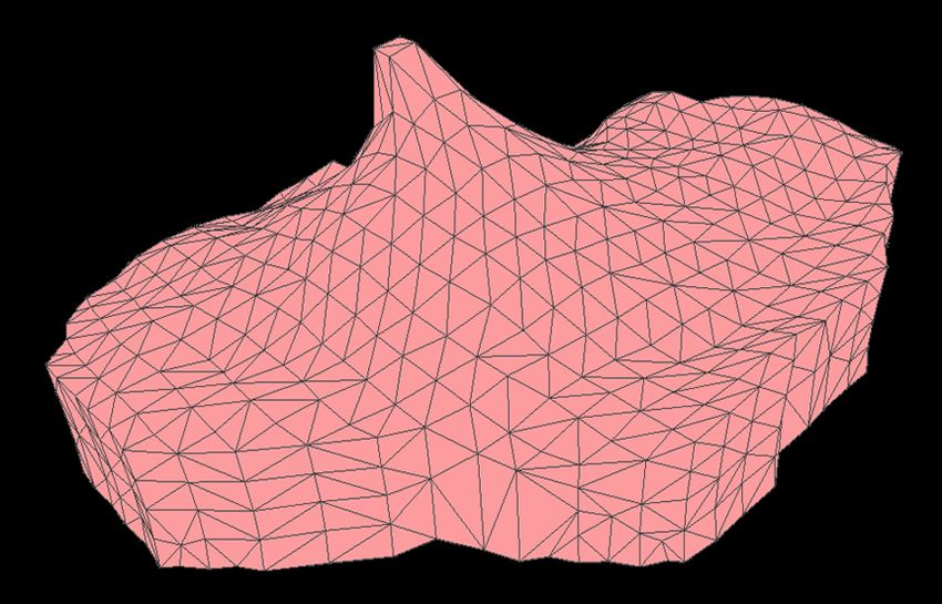
You can also read