Heading direction with respect to a reference point modulates place-cell activity - bioRxiv
←
→
Page content transcription
If your browser does not render page correctly, please read the page content below
bioRxiv preprint first posted online Oct. 2, 2018; doi: http://dx.doi.org/10.1101/433516. The copyright holder for this preprint
(which was not peer-reviewed) is the author/funder, who has granted bioRxiv a license to display the preprint in perpetuity.
                                   All rights reserved. No reuse allowed without permission.

    Heading direction with respect to a reference point modulates
    place-cell activity

                    1                  2                  1                 1                1,4,6,7                   1,3,4,5,6,7
    Jercog P.E. , Ahmadian Y. , Woodruff C. , Deb-Sen R. , Abbott L.F.                                 , Kandel E.R.

    1
      Dept. of Neuroscience, College of Physicians and Surgeons of Columbia University, New York, NY 10032, USA
    2
      Institute of Neuroscience, Dept. of Biology and Mathematics, University of Oregon, Eugene, OR 97401, USA
    3
      Dept. of Psychiatry, College of Physicians and Surgeons of Columbia University, New York, NY 10032, USA
    4
      Dept. of Physiology and Cellular Biophysics, College of Physicians and Surgeons of Columbia University, New
               York, NY 10032, USA
    5
      Howard Hughes Medical Institute at Columbia University, New York, NY 10032, USA
    6
      Zuckerman Mind Brain Behavior Institute, Columbia University, New York, NY 10027, USA
    7
      Kavli Institute for Brain Science, Columbia University, New York, NY 10032, USA

    Abstract

    Utilizing electrophysiological recordings from CA1 pyramidal cells in freely moving mice, we
    find that a majority of neural responses are modulated by the heading-direction of the animal
    relative to a point within or outside their enclosure that we call a reference point. Our findings
    identify a novel representation in the neuronal responses in the dorsal hippocampus.

    Introduction

    Successful navigation requires knowledge of both location and direction, quantities that must
    be computed from self-motion and environmental cues. Place cells in the dorsal
    hippocampus (O’Keefe and Dostrovsky 1971), grid cells in entorhinal cortex (Fyhn et al
    2004), and head-direction cells in various brain regions (Wiener et al 1989, Taube et al
    1990, Mueller et al 1994, Sargolini et al 2006, Rubin et al 2014) are leading candidates for
    providing neural representations of location and direction. Recent studies have revealed
    goal-oriented cells hippocampus of the bat tuned to the direction of motion relative to
    rewarded locations within an environment (Sarel et al 2017; see also Hoydal et al 2018).
    Here, we provide evidence that CA1 neurons in mice exhibiting selectivity for location are
    also modulated by heading direction relative to a reference point located inside or outside
    their enclosure.

    Results

    We recorded 1244 neurons in the dorsal region of both hippocampi (area CA1;Methods) in
    12 C57BL/J6 mice recorded daily during 4 sessions of 10 minutes each over a period of 10
    days. The analysis presented here is based on 697 neurons that satisfied a set of minimal
    response and sampling criteria (Methods). During each session, food deprived animals
    foraged freely within a 50 by 50 cm enclosure. In addition to monitoring the location of the
    animal (x, y), we tracked its absolute heading-direction angle (H), defined as heading
    direction relative to a fixed orientation in the room (coinciding with a cue card on one wall).
    The enclosure was divided into 100 square bins (5 cm by 5 cm each) and the heading angle
    into 10 bins of 36° each. Firing rates of the recorded neurons were computed for each bin,
    yielding firing-rate data r(x, y, H).
bioRxiv preprint first posted online Oct. 2, 2018; doi: http://dx.doi.org/10.1101/433516. The copyright holder for this preprint
(which was not peer-reviewed) is the author/funder, who has granted bioRxiv a license to display the preprint in perpetuity.
                                   All rights reserved. No reuse allowed without permission.

    Figure 1: Heading-direction modulation. a) Firing rate as a function of location for a typical place
    cell (left). Colors from blue to red indicate low to high firing rates. Percent variance across neurons
    explained by location tuning (right). b) Example of heading-direction tuning in one neuron. Radius of
    curve is proportional to the firing rate. c) Tuning of firing rate for heading direction shown as rate-
    weighted sums of heading direction vectors within each bin. Place fields are also shown, as in a. Red
    circles are the centers of mass of the place fields. White squares denote bins with average firing rates
    too low to be included in the analysis of directional modulation. d) Average tuning strengths of
    heading-direction modulation across bins for actual and randomly reshuffled data. Tuning strength is
    defined as the lengths of vectors computed as in c, averaged over bins for each neuron. For
    surrogate data, head-direction angles were randomly reshuffled in each bin. Green circle denotes the
    means of both distributions. e, f) Correlation between the preferred heading direction (pref. HD) and
    either the direction of motion (top) or the velocity (bottom) for actual compared to shuffled data.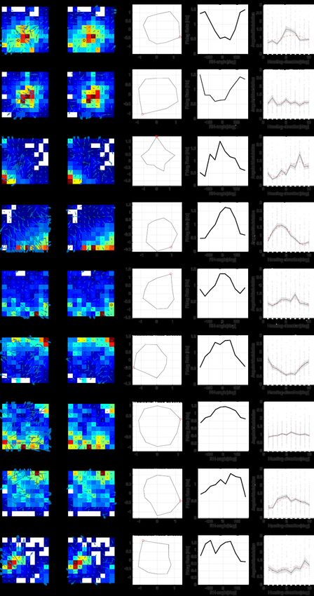
bioRxiv preprint first posted online Oct. 2, 2018; doi: http://dx.doi.org/10.1101/433516. The copyright holder for this preprint
(which was not peer-reviewed) is the author/funder, who has granted bioRxiv a license to display the preprint in perpetuity.
                                   All rights reserved. No reuse allowed without permission.

    Responses of most of the recorded neurons were modulated by the location of the animal,
    and many would be classified as place-cells (Fig.1a (left)). Additional modulation of the
    activity of hippocampal neurons by heading direction relative to a fix orientation within the
    experimental room has been reported (Fig.1b Wiener et al 1989, Rubin et al 2014), although
    confounds associated with animal behavior have challenged the interpretation of this effect
    (Mueller et al 1994). Because place tuning accounts for a relatively small percentage of the
    variance of our recorded neurons (less than 50%, and often considerably less;Fig.1a (right)),
    we investigated modulation of the neuronal responses by heading direction defined more
    generally, that is, relative to various points in the environment.

    A conventional place-cell description is obtained by averaging the rates r(x, y, H) over
    heading angles yielding a place-modulated rate r(x, y). To examine directional modulation,
    we considered the ratio R(x, y, H) = r(x, y, H)/r(x, y) for all bins that have firing rates greater
    than 0.5 Hz (we eliminated smaller rates to avoid numerical problems with small
    denominators; results did not change when we changed this cutoff). We multiplied unit
    vectors corresponding to angles centered within each heading-direction bin by the
    associated rate ratio R(x, y, H) and averaged to compute a preferred heading vector for each
    bin (Fig.1c; Methods; for further examples see SupplFig.1). We quantified heading-direction
    tuning by computing the lengths of these preferred heading vectors and averaging them over
    bins to obtain a tuning strength for each neuron. We then compared tuning strengths
    computed from the data with results obtained by randomly shuffling the heading angles
    within each bin (Methods). In this comparison, 70% of the recorded neurons have stronger
    modulation by heading direction for the data than for the shuffled data, a highly statistically
    significant effect (Fig.1d; p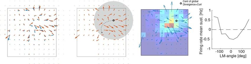
bioRxiv preprint first posted online Oct. 2, 2018; doi: http://dx.doi.org/10.1101/433516. The copyright holder for this preprint
(which was not peer-reviewed) is the author/funder, who has granted bioRxiv a license to display the preprint in perpetuity.
                                   All rights reserved. No reuse allowed without permission.

    point. We used a subtraction procedure to assure that the average of the modulation over H
    is equal to 1 to remove biases (Methods).

    Tuning strengths, defined as in figure 1d, were computed by multiplying the rates r(x, y) by
    the modeled direction modulation, and these were then compared between actual and
    shuffled data. A majority of neurons (70%) showed stronger tuning for actual than shuffled
    data (Fig.2b). We also computed the percent variance accounted for by the modulated rates
    and compared it to the percentages accounted by the direction-unmodulated rates r(x, y).
    Many neurons showed a substantial increase in explained variance when the directional-
    modulation described by the model was included (Fig.2c&d). This model describes the
    directional tuning of many neurons quite accurately (Fig.2e).

    Figure 2: Model of modulation by heading-direction relative to a reference point.
    a) Definitions of the reference point and reference-heading angle. b) Reference-heading (RH)
    angle tuning for the recorded population of neurons compared to the tuning for surrogate data
    with randomly shuffled heading directions. Green circle is defined as in figure 1. c) Variance
    explained by the model with both reference-heading angle and place modulation compared to a
    purely spatial description. d) Histogram of the fractional change in variance, defined as the
    change in variance divided by the variance explained solely by place modulation. e) Examples of
    model fit (red line) across heading-angle bins for 5 different neurons. Black lines are means and
    shaded areas are standard error of the mean for the data. The red line is an average of the
    model over spatial bins. Grey points show all the data for each neuron.

    The fitting process provides a distribution of the modulation strengths (g; Fig.3a), the
    preferred reference-heading directions (!! ; Fig.3b), and the x and y coordinates of the
    reference point (Fig.3c). The firing rates of most of the neurons are maximally enhanced
    when the animal moves toward the reference point (! p = 0). Reference points for the majority
    of the neurons (60%) are inside the enclosure, 8% are outside but close to the enclosure,
    and 32% are distal (Fig.3d). Neurons with distal reference points are effectively modulated
    by the absolute heading direction of the animal (Suppl.Fig.3). For neurons with reference
    points inside the enclosure, we found no correlation between the location of the reference
    point and the center of the place field (Fig.3e).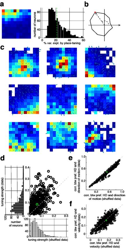
bioRxiv preprint first posted online Oct. 2, 2018; doi: http://dx.doi.org/10.1101/433516. The copyright holder for this preprint
(which was not peer-reviewed) is the author/funder, who has granted bioRxiv a license to display the preprint in perpetuity.
                                   All rights reserved. No reuse allowed without permission.

    We also utilized an independent method to search for reference point locations based on an
    iterative algorithm that finds the centers of divergences and curls from the heading direction
    responses vector fields (Suppl.Fig.4). We found that the points of maximum divergence and
    curl generated by this method provide a good estimation of the reference point locations
    fitted by the model, coinciding in a majority of the cells within the same quadrant of the
    enclosure (Suppl.Fig.5).

    Figure 3: Fitted model parameters across neurons. a) Histogram of the amplitude of the angular
    modulation. b) Histogram of angle of the preferred reference-heading direction. c) Reference point
    locations inside and outside the enclosure. The the square in the center of the panel indicates the
    enclosure. Distal reference points do not appear in this figure. d) Histogram of the distances of
    reference points (RP) from the center of the enclosure. e) Coordinates of the reference points (x-left,
    y-right) compared to the coordinates of the centers of the place fields for each neuron.

    Conclusions

    We find that the firing rates of the majority of neurons in the CA1 region of the dorsal
    hippocampus are modulated by the heading direction of the animal relative to a reference
    point in the environment. The majority of the neurons have a higher response when the
    animal moves towards the location of the reference point. This generalizes the idea of goal-
    (Sarel et al 2017) and object-oriented (Hoydal et al 2018) neurons to a more abstract
    relationship of heading direction to an unmarked point in the environment, the reference
    point, and it accounts for previously reported head-direction cells (Wiener et al 1989) as
    neurons with reference points located far from the enclosure.
bioRxiv preprint first posted online Oct. 2, 2018; doi: http://dx.doi.org/10.1101/433516. The copyright holder for this preprint
(which was not peer-reviewed) is the author/funder, who has granted bioRxiv a license to display the preprint in perpetuity.
All rights reserved. No reuse allowed without permission.
References
Fyhn M, Molden S, Witter MP, Moser EI, Moser MB. Spatial representation in the entorhinal
cortex. Science. 2004 Aug 27;305(5688):1258-64.
Hoydal OA, Skytoen ER, Moser M-B, Moser, EI (2018) Object-vector coding in the medial
entorhinal cortex. BioR!iv doi: doi.org/10.1101/286286.
Muller RU, Bostock E, Taube JS, Kubie JL (1994) On the directional firing properties of
hippocampal place cells. J Neurosci 14:7235–7251.
O’Keefe J, Dostrovsky J (1971) The hippocampus as a spatial map. Prelim-
inary evidence from unit activity in the freely-moving rat. Brain Res 34:171–175.
Rubin, A, Yartsev, MM and Ulanovsky, N, 2014. Encoding of head direction by hippocampal
place cells in bats. J Neurosci 34:1067-1080.
Sarel A, Finkelstein A, Las L, Ulanovsky N (2017) Vectorial representation of spatial goals in
the hippocampus of bats. Science 355:176-180.
Sargolini, F, Fyhn, M, Hafting, T, McNaughton, BL, Witter, MP, Moser, MB and Moser, EI,
2006. Conjunctive representation of position, direction, and velocity in entorhinal cortex.
Science, 312(5774), pp.758-762.
Taube JS, Muller RU, Ranck JB (1990). Head-direction cells recorded from the
postsubiculum in freely moving rats. I. Description and quantitative analysis. J Neurosci 10:
420–435.
Wiener SI, Paul CA, Eichenbaum, H (1989) Spatial and behavioral correlates of
hippocampal neuronal activity. J Neurosci 9:2737-2763.
Acknowledgments
PEJ’s research supported by the Mathers Foundation and Swartz Program in Computational
Neuroscience.
YA’s research supported by the Swartz Program in Computational Neuroscience.
LFA's research supported by NSF NeuroNex Award DBI-1707398, the Gatsby Charitable
Foundation and the Simons Collaboration for the Global Brain.
ERK’s research supported by the Mathers and Howard Hughes Medical Institute.
Contributions
PEJ designed the experiment, did the surgeries for the recordings, analyzed the data and
helped write the manuscript; YA helped designing statistical tests; CW ran behavioral
experiments; RD performed data pre-processing; LFA developed the model, analyzed the
data and wrote the manuscript; ERK helped with the design of the experiment and writing of
the manuscript and supervised the project.bioRxiv preprint first posted online Oct. 2, 2018; doi: http://dx.doi.org/10.1101/433516. The copyright holder for this preprint
(which was not peer-reviewed) is the author/funder, who has granted bioRxiv a license to display the preprint in perpetuity.
All rights reserved. No reuse allowed without permission.
Methods
Subjects
Data was recorded from 12 male C57BL/6J mice. In 4 mice, 1 microdrive with a bundle of 4
tetrodes was implanted in the right hippocampal area CA1, and the other 8 mice were
implanted with two microdrives each, with 4 tetrodes in both hemispheres (area CA1:
1.8mmDL, 1.8mmRC, ~1.1mm deep). Mice were 6-9 month old (30-34g.) at the time of the
implantation surgery. After surgery, all mice were individually housed under 12 hr light/dark
cycle and provided water ad libitum and one food pellet overnight (maintaining the same
body-weight as prior to the implantation (+ the implant)). All housing procedures conformed
to National Institute of Health (NIH) standards using protocols approved by the Institutional
Animal Care and Use Committee (IACUC).
Electrode implantation and surgery
Custom-made, reusable microdrives (Axona) were constructed by attaching an inner (23 ga)
stainless steel cannula to the microdrive’s movable part to allow inserting the electrode
reliably at 10 microns steps. An outer (19 ga) cannula covered the exposed tetrode section
from the dura to the inner cannula. Tetrodes were built by twisting four 17 µm thick platinum-
iridium wires (California wires) and then heat bonded them. Four such tetrodes were inserted
into the inner cannula of the microdrive and connected to the wires of the microdrive. Prior to
surgery, the tetrodes were cut to an appropriate length and plated with a platinum/gold
solution with additives (Ferguson J.E. et al 2009) until the impedance dropped to 80–100
KΩ. All surgical procedures were performed following NIH guidelines in accordance with
IACUC protocols. Mice were anesthetized with a mixture of 0.11 ml of Ketamine and
Xylazine (100 mg/ml, 15 mg/ml, respectively) per 10 g body weight. Once under anesthesia,
mice were fixed to the stereotaxic unit with head restrained using ear-bars. The head was
shaved and an incision was made to expose the skull. Ten jeweler's screws were inserted
into the skull to support the microdrive implant. Two of these screws were soldered to wires
and screwed until they pierced the Dura, which served as a ground/reference for EEG
recordings (one in olfactory-bulb and one in the cerebellum). A 2 mm hole was made in the
skull at position 1.8 mm medio-lateral and 1.8 mm antero-posterior to bregma junction.
Tetrodes were lowered to about 0.7 mm from the surface of the brain (dura). Dental cement
was spread across the exposed skull and secured to the microdrive. Any loose skin was
sutured back in place to cover the wound. Mice were given Carprofen (5 mg/kg) post-
operatively to reduce post-procedure pain. Mice usually recovered within a day after the
tetrodes were lowered.
Histology
To determine the exact final position of the tetrodes in a given animal we performed Nissl
dye staining on hippocampal slices. After the experiment was concluded, mice were
anesthetized with an overdose of 0.5 ml Ketamine and Xylazine solution (100 mg/ml and 15
mg/ml, respectively) and intra-cardiac perfused with 40 ml of 4% PFA solution, immediately
after the tetrodes were retracted before mice were decapitated. The skull was cut open from
the bottom of the head to expose the brain, which was gently removed and stored in 4%
PFA solution for 24 hr in a shaker. The brain was coronally sliced in 30 µm thick sections
using a cryostat at -13˚C. The sections were stained with fluorescent Nissl dye (Neurotrace)
and mounted onto a slide. The brain sections were viewed under a high magnification
microscope, and digital pictures of the slices were taken.bioRxiv preprint first posted online Oct. 2, 2018; doi: http://dx.doi.org/10.1101/433516. The copyright holder for this preprint
(which was not peer-reviewed) is the author/funder, who has granted bioRxiv a license to display the preprint in perpetuity.
All rights reserved. No reuse allowed without permission.
Experimental methods
After animals recovered their normal weight a few days post-surgery, the electrodes were
connected to an amplifier to detect single cells. Tetrodes were lowered ~12.5microns twice a
day (6 hrs. apart) until the number of recorded cells was maximized (this process took
between seven to ten days). After the depth of the electrode was optimal, we waited 3-8
days for recording stabilization. Animals were food deprived for four hours before the
recording sessions throughout the length of the experiment (7-35 days). Animal’s were
reconnected to 16 or 32 channels for every single session of ten minutes and introduced in
the same region of the arena relative to the recording room in each of the three
environments. Each environment is approximately 50cm wide with walls that are 40 cm in
height. All three environments present a cue card on the internal side of the enclosure with
the same orientation relative to the room for all three environments (north on our plots in fig.
1) to act as a reference point for navigation. Environment A was a square enclosure with
black walls and white floor that has ground food (vanilla cookie) spread over the surface of
the floor and also a small pellet ~10cm away from the S-E corner of the environment.
Environment B was a circular enclosure with black walls and brown textured floor with
ground food (cocoa flavored puffed rice) spread over the surface. Environment C was a
circular enclosure with white walls and floor and no food. We used these differences in
shape and reward distribution to enhance the animal’s ability to differentiate between the
environments. Animals were release to freely explore the environments and eat the food. For
this paper, we only used the data from Environment A.
Recordings were done with Neuralynx amplifiers: Lynx-8, with a total of 16 to 32 channels
depending on the success of the electrode’s implantation surgery. Data was collected in
continuous format at a 30 kHz sampling rate and then pre-processed using NDManager
(Hazan et al 2006). High and low frequencies were separated and spike wave-forms were
extracted for cell identification. Cell clusters were computed using the EM algorithm
implemented in the KlustaKwik software (KD Harris et al 2000) over the concatenated data
of the 12 sessions within a day for each animal. Human inspection over each cluster was
done using Klusters software (Hazan et al 2006). Spike times and animal trajectories were
transformed into Matlab objects and data analysis was performed using this platform.
Before analyzing the data, the length of the useful portion of the experiment over days for a
given mouse was determine based on our criteria of recording stability. Because we wanted
“in principle” to follow the same cells over days, we established the following criteria for
determine stability: for each cell we chose the channel with the largest spike-waveform
fluctuation over the 4 channels on a given tetrode. We then computed over that channel the
mean wave-form in a vector of 40 discretized points (at 30 kHz sampling rate). We
calculated the peak amplitude of the mean waveform over all cells and also its standard
deviation. We then compared the distributions of peak wave-forms for each cell across days
using a t-test for two distributions with different means and standard deviations; when these
distributions became statistically different we stopped using the data from that day on, for
that particular animal.
Data analysis
After units were isolated, cells were considered for the analysis if their average firing rate
across the 4 sessions within a day was higher than 0.1 Hz. This threshold left out
approximately 2% of the cells. To avoid spikes that are not correlated with mouse position
due to pre-play or re-play (e.g. nonspecific spatial firing when animals are not moving withinbioRxiv preprint first posted online Oct. 2, 2018; doi: http://dx.doi.org/10.1101/433516. The copyright holder for this preprint
(which was not peer-reviewed) is the author/funder, who has granted bioRxiv a license to display the preprint in perpetuity.
All rights reserved. No reuse allowed without permission.
the box; Nádasdy et al 1999, Diba & Buszaki 2007, Davidson et al 2009), we only kept
frames in which the animal was moving faster than 4 cm/sec. This threshold was obtained by
scoring movies and avoid frames where animals were not moving their bodies but just their
heads. We called these bins: “effective time bins”. For each spatial and angular bin (x,y,H, 3-
dim, 10 bins per dimension, 1000 total spatial bins), we utilized the effective time bins to
count the spikes occurring in each of bin. We then computed the mean-rate for each bin as
the spike counts for each of the samples from each visit of the animal to a given spatial bin.
We then divided the mean spike count by the size of the time bin (1/30 s) defined by our
maximum accuracy for predicting animal position and heading-direction. Heading-direction
(H) is the angle in 2-D between the position of the animal at time !! and time !!!! . We also
monitored the head direction of the animal measured by the positions of two LEDs attached
to the pre-amplifier connected to the mouse tetrode boards, but this variable was not as well
defined as the heading-direction (H) due to the many degrees of freedom of the animal’s
head while moving during the session. We use the same definition of heading-direction as
Sarel et al 2017.
Model fitting
Our proposed model describes the angular dependency of the firing rate for all heading-
direction angles and spatial bins. We binned each spatial and angular coordinate into 10
bins to have sufficient statistics within each bin. We used averages of 72 samples per bin
during 40 minute recording per day. Position and heading-direction was computed at the
video camera frame rate of 30 Hz. Heading direction was computed from the change in the
animal’s position between two video recording frames (previous and current frame).
Because the model fit heading-direction modulation, we divided the firing rate for all three
dimensions by the spatial dependence only, assuming that the modulation of the firing rate
by heading-direction is multiplicative. Thus, we considered the quantity
!(!, !, !) = ! (!, !, !)/!(!, !)
Over the entire article we only considered spatial bins in which average firing rates were
larger than 0.5 Hz (we call this the “min-criteria”). We then used neurons that satisfy the
following conditions: minimum number of spatial bins that satisfy the min-criteria = 10;
minimum range of heading-direction angles to which the cell is responsive to = 50 deg. We
also reproduced the same results with lower thresholds of minimum firing rate (0.1Hz).
The model has a periodic dependence on the angle between the heading-direction of the
animal’s trajectory and the location of the reference point (See Fig.1b)
!!"#$% (!, !, !) = 1 + !(! − !), where ! = !"#(! − !! ) and ! = ![!]!
! = arctan !!"#.!"#$% − !, !!"#.!"#$% − ! , and imposing !!"#$% !, !, ! > 0
We fitted the values of !,!! , !!"#.!"#$% , !!"#.!"#$% by minimizing the variance of the model
with respect to the data: ! = !"#[!!"#$% (!, !, !) − !(!, !, !)].
We minimized the variance utilizing an unconstrained nonlinear optimization procedure: the
fminsearch function from MATLAB. For the initial parameter estimates we used: !=0;!! =0;
!!"#.!"#$% =Place-cell’s center of mass X-coord, !!"#.!"#$% =Place-cell’s center of mass Y-
coord.bioRxiv preprint first posted online Oct. 2, 2018; doi: http://dx.doi.org/10.1101/433516. The copyright holder for this preprint
(which was not peer-reviewed) is the author/funder, who has granted bioRxiv a license to display the preprint in perpetuity.
All rights reserved. No reuse allowed without permission.
Statistical tests
In figure 1a, we computed the variance explained by a place description to describe how well
the mean rate over all angular bins explain the neural activity,
!"#[!(!, !)]
Variance Explained by Place without tuning = 1 −
!"#[!(!, !, !)]
In figure 1b. we show, in a polar plot, the average rate for each of the 10 heading-direction
angles, averaged over the entire experiment.
For figure 1d,e and f, we performed a chi-square goodness-of-fit test, and we rejected the
hypothesis that the distributions in the X and Y axis were coming from the same distribution
with the actual values computed being pvalue=6x10-14, pvalue=2x10-36, pvalue=0.028 respectively.
In figure 2b, we performed a chi-square goodness-of-fit test, and we rejected the hypothesis
that the distributions in the X and Y axis were coming from the same distribution with the
actual value computed being pvalue=4x10-15.
In figure 2c, we compared the variance explained by the place-tuning versus the variance
explained by including reference-heading (RH) angular dependence where the reference
point was fitted by the model:
!"#[!(!, !)]
Variance Explained by Place − tuning = 1 −
!"#[!(!, !, !)]
!"#[!(!, !)!model (!, !, !)]
Variance Explained including RH tuning = 1 −
!"#[!(!, !, !)]
References for Methods
J.E. Ferguson, C. Boldt, and A.D. Redish (2009) Creating low-impedance tetrodes by
electroplating with additives 2009 Sens Actuators A Phys.;156(2):388-393.
L. Hazan, M. Zugaro, G. Buzsáki (2006). Klusters, NeuroScope, NDManager: a Free
Software Suite for Neurophysiological Data Processing and Visualization, J. Neurosci.
Methods; 155:207-216.
Harris KD, Henze DA, Csicsvari J, Hirase H, Buzsáki G. (2000) Accuracy of tetrode spike
separation as determined by simultaneous intracellular and extracellular measurements. J
Neurophysiol.; 84(1):401-14.bioRxiv preprint first posted online Oct. 2, 2018; doi: http://dx.doi.org/10.1101/433516. The copyright holder for this preprint
(which was not peer-reviewed) is the author/funder, who has granted bioRxiv a license to display the preprint in perpetuity.
All rights reserved. No reuse allowed without permission.
Supplementary Figure 1: Normalized vector fields obtained from the heading direction
with higher vector strength on each spatial bin. Top, Correlation of the vector fields for
the raw data, and for shuffle data to compare the values of correlations that we would obtain
at chance on a vector field of 10 by 10 bins. Correlation of the vector fields for the raw data
versus shuffle, show a population of cells that could not be explain by randomly adding
directions on the place cell field modulated by the behavior of the animal (pink region)
Bottom, example of normalized vectors fields to visualize organization of prefer heading
direction response. The structures in some neurons are global and give information of a
perturbation like a curl, a divergence or a saddle-node at the other side of the arena.bioRxiv preprint first posted online Oct. 2, 2018; doi: http://dx.doi.org/10.1101/433516. The copyright holder for this preprint
(which was not peer-reviewed) is the author/funder, who has granted bioRxiv a license to display the preprint in perpetuity.
All rights reserved. No reuse allowed without permission.
Supplementary Figure 2: Non-uniformities in heading direction distribution per spatial
bin, does not explain the angular tuning of neural responses. Each spatial bin has a
distribution of heading directions manifesting the directionality of the trajectories when the
animal visited that given spatial bin. Left: The angular distribution per bin is not uniform and
is represented by the map on red tones on the top-left plot. The more red is the bin, the less
uniform are the visits in a session of 40min. The distribution over the bins for the whole
environment is represented by the mean and the std of distributions per bin, as a circle in the
plot for all sessions. Red circle is a “average” sessions represented on the map above. Right:
mean and +/- std of vector-strength for the populations of neurons when are included spatial
bins with different levels of heading direction coverage, starting by the bins with the best 10%
uniformity, until reaching the totality of bins indicated by 100%. As is it shown, the angular
tuning decreases when bins with lower uniformity are included in the computation of the
vector-strength. This rules out the argument by Mueller et al 1994, that the angular tuning in
dorsal hippocampal neuronal responses is an artifact of the low angular coverage of certain
bins of the environment close to the borders of the box. If any, including this bins into the
computation of the angular tuning, decreases then tuning as it is shown here.bioRxiv preprint first posted online Oct. 2, 2018; doi: http://dx.doi.org/10.1101/433516. The copyright holder for this preprint
(which was not peer-reviewed) is the author/funder, who has granted bioRxiv a license to display the preprint in perpetuity.
All rights reserved. No reuse allowed without permission.
Supplementary Figure 3: Examples of neuronal response for reference point tending to
infinity generated by our model. (Top-left) If the reference point is within the arena and
with phase angle ( θp =0) neural response relative to the heading-direction is maximal when
animal faces the reference point. (Top-from-left to-right) If the reference point moves from
the center of the arena, the heading-direction vector field tend to point to the reference point
reaching the point of a parallel field with reference point at the infinity. Heading-direction
circular histogram shows the evolution towards a traditional pure Head-direction neuronal
response. (Bottom-from-left to-right) as on the top row heading-direction response tend to
behave as traditional head-direction cells when reference point moves to infinity. In these
examples the θp is equal to 90, so the maximal neural response is when the animal moves
perpendicular to the reference point.bioRxiv preprint first posted online Oct. 2, 2018; doi: http://dx.doi.org/10.1101/433516. The copyright holder for this preprint
(which was not peer-reviewed) is the author/funder, who has granted bioRxiv a license to display the preprint in perpetuity.
All rights reserved. No reuse allowed without permission.
Supplementary Figure 4: Computing the center of the divergence and the curl of the
heading-direction responses’ vector field. Far-left: vector field generated by the vectors of
the best heading direction responses in each bin (blue arrows) for all bins in the arena (10 by
10). Red arrows are the smoother version of the original vector field (blue) convolved with a
2-D gaussian filter for vector’s angle and length. This filter gives a 2 extra bins of edging.
Left: once the vector field is smoothed, the location of the curl and the divergence (which are
local descriptors of the field) are computed within a disc around the possible candidate,
starting from the center of the arena and running in an iterative manner, in order to find the
center of divergence+curl for a large part of the field. We will call this, the global center of
divergence and curl for the neural response (black circle). Right: superposition of the
heading direction vector field with the place-field in x-y coordinates. Far-right: neural
response for the angle dependence relative to the center of the global divergence+curl.
Supplementary Figure 5:Curl+Divergence iterative method coincide with the reference
point location obtained by our proposed model. The method described on Suppl.Fig.4 to
find the Curl and Divergence of the heading-direction neural response provides candidates
for the singularities related the reference points. The estimation of the reference point location
from the two methods predicts this singular points to be within the same environment
quadrant. The error between the methods is not small, but is mainly originated by the fact that
we can only compute Curl and Divergence within the enclosure. We also show that this
prediction is not random, since the distribution of the Curl+divergence distance to the
place-fields center of mass (another comparable point within the enclosure) is much higher.bioRxiv preprint first posted online Oct. 2, 2018; doi: http://dx.doi.org/10.1101/433516. The copyright holder for this preprint
(which was not peer-reviewed) is the author/funder, who has granted bioRxiv a license to display the preprint in perpetuity.
All rights reserved. No reuse allowed without permission.
Supplementary Figure 6: RH tuning for all cells included in Fig1c to show diversity in the
RH-tuning responses.You can also read