A Robust and Scalable Approach to Face Identi cation
←
→
Page content transcription
If your browser does not render page correctly, please read the page content below
A Robust and Scalable Approach to
                 Face Identification

            William Robson Schwartz, Huimin Guo, Larry S. Davis

     University of Maryland, A.V. Williams Building, College Park, MD, 20742
                       {schwartz,hmguo,lsd}@cs.umd.edu

      Abstract. The problem of face identification has received significant
      attention over the years. For a given probe face, the goal of face identifi-
      cation is to match this unknown face against a gallery of known people.
      Due to the availability of large amounts of data acquired in a variety of
      conditions, techniques that are both robust to uncontrolled acquisition
      conditions and scalable to large gallery sizes, which may need to be in-
      crementally built, are challenges. In this work we tackle both problems.
      Initially, we propose a novel approach to robust face identification based
      on Partial Least Squares (PLS) to perform multi-channel feature weight-
      ing. Then, we extend the method to a tree-based discriminative structure
      aiming at reducing the time required to evaluate novel probe samples.
      The method is evaluated through experiments on FERET and FRGC
      datasets. In most of the comparisons our method outperforms state-
      of-art face identification techniques. Furthermore, our method presents
      scalability to large datasets.

      Key words: Face Identification, Feature combination, Feature selec-
      tion, Partial Least Squares.

1   Introduction

The three primary face recognition tasks are verification, identification, and
watch list [1]. In verification, the task is to accept or deny the identity claimed
by a person. In identification, an image of an unknown person is matched to
a gallery of known people. In the watch list task, a face recognition system
must first detect if an individual is on the watch list. If the individual is on the
watch list, the system must then correctly identify the individual. The method
described in this paper addresses the identification task.
    Previous research has shown that face recognition under well controlled ac-
quisition conditions is relatively mature and provides high recognition rates even
when a large number of subjects is in the gallery [2, 3]. However, when images
are collected under uncontrolled conditions, such as uncontrolled lighting and
changes in facial expressions, the recognition rates decrease significantly.
    Due to the large size of realistic galleries, not only the accuracy but also the
scalability of a face identification system needs to be considered. The main scala-
bility issues are the following. First, the number of subjects in the gallery can be
quite large, so that common search techniques, such as brute force nearest neigh-
bor, employed to match probe faces do not scale well. Second, in applications
such as surveillance and human computer interaction, in which new subjects are
added incrementally, the necessity of rebuilding the gallery models every time a
new subject is added compromises the computational performance of the system.
    We tackle both problems. In order to reduce the problems associated with
data collected under uncontrolled conditions, we consider a combination of low-
level feature descriptors based on different clues (such approaches have provided
significant improvements in object detection [4, 5] and recognition [6]). Then, fea-
ture weighting is performed by Partial Least Squares (PLS), which handles very
high-dimensional data presenting multicollinearity and works well even when
very few samples are available [5, 7–9]. Finally, a one-against-all classification
scheme is used to model the subjects in the gallery.
    To make the method scalable to the gallery size, we modify the one-against-
all approach to use a tree-based structure. At each internal node of the tree,
a binary classifier based on PLS regression is used to guide the search for the
matching subject in the gallery. The use of this structure provides substantial
reduction in the number of comparisons when a probe sample is matched against
the gallery and also eliminates the need for rebuilding all PLS models when new
subjects are added to the gallery.
    Our proposed face identification approach outperforms state-of-art techniques
in most of the comparisons considering standard face recognition datasets, par-
ticularly when the data is acquired under uncontrolled conditions, such as in
experiment 4 of the FRGC dataset. In addition, our approach can also handle
the problem of insufficient training data – results show high performance when
only a single sample per subject is available. Finally, due to the incorporation
of the tree-based structure, a significant number of comparisons can be saved
when compared to approaches based on brute force nearest neighbor search.

2   Related Work

Detailed discussion of face recognition and processing can be found in recent and
comprehensive surveys written by Tolba et al. [2] and Zhao et al. [3].
    Most approaches to face recognition can be divided into two categories: holis-
tic matching methods and local matching methods [10]. Methods in the former
category use the whole face region to perform recognition and includes techniques
such as subspace discriminant analysis, SVM, and AdaBoost; these may not cope
well with the generalizability problem due to the unpredictable distribution of
real-world testing face images. Methods in the latter category first locate several
facial features and then classify the faces according to local statistics.
    Local binary patterns (LBP) and Gabor filters are descriptors widely used in
face recognition. LBP is robust to illumination variations due to its invariance
to monotonic gray-scale changes and Gabor filters are also robust to illumina-
tion variations since they detect amplitude-invariant spatial frequencies of pixel
gray values [10]. There are several combinations or variations based on these
descriptors that have been used for face recognition [6, 11–13].
    Most recently developed face recognition systems work well when images are
obtained under controlled conditions or when the test image is captured un-
der similar conditions to those for the training images. However, under varying
lighting or aging effects, their performance is still not satisfactory. To perform
recognition under fairly uncontrolled conditions Tan and Triggs [14] proposed a
preprocessing chain for illumination normalization. They used the local ternary
patterns and a Hausdorff-like distance measure. Holappa [15] used local binary
pattern texture features and proposed a filter optimization procedure for illumi-
nation normalization. Aggarwal [16] presented a physical model using Lambert’s
Law to generalize across varying situations. Shih [17] proposed a new color space
LC1 C2 as a linear transformation of the RGB color space.
    Another challenge is that most current face recognition algorithms perform
well when several training images are available per subject; however they are still
not adequate for scenarios where a single sample per subject is available. In real
world applications, one training sample per subject presents advantages such as
ease of collect galleries, low cost for storage and lower computational cost [18].
Thus, a robust face recognition system able to work with both single and several
samples per subject is desirable. In [19], Liu et al. proposed representing each
single (training, testing) image as a subspace spanned by synthesized shifted
images and designed a new subspace distance metric.
    Regarding the scalability issues discussed previously, there is also previous
work focused on scaling recognition systems to large datasets. In [20] a technique
for combining rejection classifiers into a cascade is proposed to speed up the
nearest neighbor search for face identification. Guo and Zhang [21] proposed the
use of a constrained majority voting scheme for AdaBoost to reduce the number
of comparisons needed.

3     Proposed Method

In this section, we first present the feature extraction process and a brief review of
partial least squares regression. Then, the proposed face identification approach
is explained in two steps. Initially, we describe the one-against-all approach, then
we describe the tree-based structure, which improves scalability when the gallery
is large and reduces the computational cost of matching probe samples.

3.1   Feature Extraction

After cropping and resizing the faces, each sample is decomposed into overlap-
ping blocks and a set of low-level feature descriptors is extracted from each block.
The features used include information related to shape (histogram of oriented
gradients (HOG) [22]), texture (captured by local binary patterns (LBP) [13]),
and color information (captured by averaging the intensities of pixels in a block).
HOG captures edge or gradient structures that are characteristic of local
shape [22]. Since the histograms are computed for regions of a given size, HOG
is robust to some location variability of face parts. HOG is also invariant to
rotations smaller than the orientation bin size.
    Local binary patterns [13] have been successfully applied in texture classifica-
tion. LBP’s characterize the spatial structure of the local image texture and are
invariant under monotonic transformations of the pixel gray values. The LBP
operator labels the pixels of an image by thresholding the 3 × 3 neighborhood
of each pixel using the center value. A label is obtained by multiplication of the
thresholded values by the binomial factors 2p followed by their addition. The
256-bin histogram of the resulting labels is used as a feature descriptor.
    Once the feature extraction process is performed for all blocks inside a
cropped face, features are concatenated creating a high-dimensional feature vec-
tor v. This vector is used to describe the face.

3.2   Partial Least Squares Regression
Partial least squares is a method for modeling relations between sets of observed
variables by means of latent variables. PLS estimates new predictor variables,
latent variables, as linear combinations of the original variables summarized in a
matrix X of predictor variables (features) and a vector y of response variables.
Detailed descriptions of the PLS method can be found in [23, 24].
    Let X ⊂ Rm denote an m-dimensional feature space and let Y ⊂ R be a 1-
dimensional space of responses. Let the number of samples be n. PLS decomposes
matrix X n×m ∈ X and vector y n×1 ∈ Y into

                                 X = TPT + E
                                  y = U qT + f

where T and U are n × p matrices containing p extracted latent vectors, the
(m × p) matrix P and the (1 × p) vector q represent the loadings and the
n × m matrix E and the n × 1 vector f are the residuals. Using the nonlinear
iterative partial least squares (NIPALS) algorithm [7], a set of weight vectors is
constructed, stored in the matrix W = (w1 , w2 , . . . , wp ), such that

                      [cov(ti , ui )]2 = max [cov(Xwi , y)]2                    (1)
                                       |wi |=1

where ti is the i-th column of matrix T , ui the i-th column of matrix U and
cov(ti , ui ) is the sample covariance between latent vectors ti and ui . After ex-
tracting the latent vectors ti and ui , the matrix X and vector y are deflated by
subtracting their rank-one approximations based on ti and ui . This process is
repeated until the desired number of latent vectors has been extracted.
   Once the low dimensional representation of the data has been obtained by
NIPALS, the regression coefficients β m×1 can estimated by

                             β = W (P T W )−1 T T y.                            (2)
remaining subjects

  subject s i

                                                                                     subjects in the gallery
                                                                                                        ...
                                                        probe sample

                                                                         response
feature extraction            feature extraction

                                                                                                         ...
                                                        feature vector
            PLS model for subject s i                                                       subject
                        (a)                                                         (b)

Fig. 1. One-against-all face identification approach. (a) construction of the PLS re-
gression model for a subject in the gallery; (b) matching of a probe sample against the
subjects in the gallery. The best match for a given probe sample is the one associated
with the PLS model presenting the highest regression response.

The regression response, yv , for a feature vector v is obtained by

                                                   yv = y + β T v                                              (3)

where y is the sample mean of y.
    Notice that even though the number of latent vectors used to create the low
dimensional representation of the data matrix X is p (possibly greater than
1), Equation 3 shows that only a single dot product of a feature vector with
the regression coefficients is needed to obtain the response of a PLS regression
model – and it is this response that is used to rank faces in a gallery. This
characteristic makes the use of PLS particularly fast for finding matches for
novel probe samples, in contrast to other methods where the number of dot
product evaluations depends on the number of eigenvectors considered, which is
quite large in general [25].

3.3     One-Against-All Approach

The procedure to learn models for subjects in the gallery g = {s1 , s2 , . . . , sn },
where si represents exemplars of each subject’s face, is illustrated in Figure 1(a)
and described in details as follows. Each si is composed of feature vectors ex-
tracted from cropped faces containing examples of the i-th subject.
    We employ a one-against-all scheme to learn a PLS discriminatory model for
each subject in the gallery. Therefore, when the i-th subject is considered, the
remaining samples g \ si are used as counter-examples of the i-th subject. In
addition, if the face dataset provides a training set we also add those samples,
(excluding samples from the subject under consideration), as counter-examples
of the i-th subject. Experiments show that the addition of training samples as
counter-examples improves recognition rates.
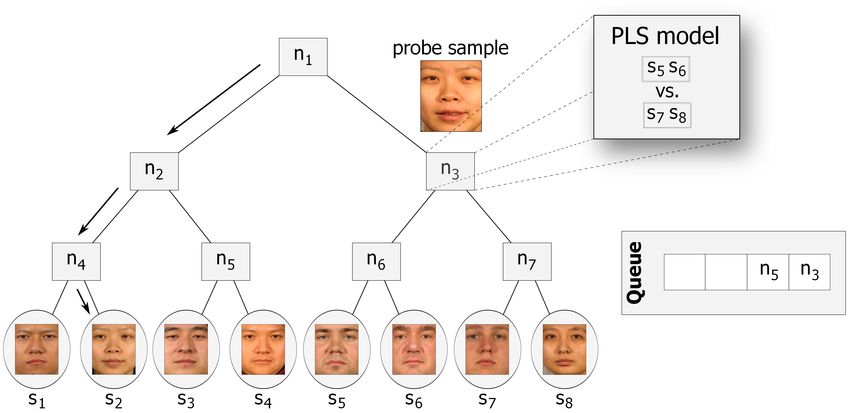
probe sample

                                               n3

      s1       s2   s3     s4      s5     s6        s7    s8

Fig. 2. Tree-based structure used to optimize the search for matches to a probe sample.
Each internal node contains a PLS regression model used to guide the search, as shown
in details for node n3 , which has a PLS model constructed so that the response directs
the search either to node n6 or n7 . In this example the first path to be traversed is
indicated by arrows (in this case, it leads to the correct match for this particular probe
sample). Alternative search paths are obtained by adding nodes that have not been
visited into a priority queue (in this example nodes n3 and n5 will be the starting
nodes for additional search paths). After pursuing a number of search paths leading
to different leaf nodes, the best match is chosen to be the one presenting the highest
response (in absolute value).

    When a one-against-all scheme is used with PLS, higher weights are at-
tributed to features located in regions containing discriminatory characteristics
between the subject under consideration and the remaining subjects.
    Once the models have been estimated for all subjects in the gallery, the PLS
regression models are stored to be later used to evaluate the responses for a probe
sample. Then, when a probe sample is presented, its feature vector is projected
onto each one of the PLS models. The model presenting the highest regression
response gives the best match for the probe sample, as illustrated in Figure 1(b).

3.4        Optimization Using a Tree-Based Structure

In terms of scalability, two drawbacks are present in the one-against-all scheme
described in the previous section. First, when a new subject is added to the
gallery, PLS models need to be rebuilt for all subjects. Second, to find the best
match to a probe sample, the feature vector representing this sample needs
to be projected onto all PLS models learned for the subjects in the gallery
(common problem faced by methods that estimate matching scores using brute
force nearest neighbor search [20]).
    To reduce the need for projecting features onto all PLS models to find the
best match for a probe sample, we construct a binary tree in which each node,
nj , contains a subset of the gallery subjects tj ⊂ g, where g = {s1 , s2 , . . . , sn }
as defined previously. A splitting procedure is used to decide which elements of
tj will belong to the left and right children of nj , assigning at least one sample
to each child. Each internal node is associated with a PLS regression model,
used afterwards to guide the search when probe samples are analyzed. In order
to build the regression model for a node, the subjects assigned to the left child
are defined to have response −1 and the subjects assigned to the right child are
defined to have response +1. The splitting procedure and the building of PLS
models are applied recursively in the tree until a node contains only a single
subject (leaf node).
   The application of the described procedure for a gallery with n subjects
results in a tree containing n leaf nodes and n − 1 PLS regression models located
on the internal nodes.
    We consider two approaches to split subjects between the children nodes.
First, a procedure that uses PCA to create a low dimensional subspace (learned
using samples from a training set) and then the K-means algorithm clusters data
into two groups, each one is assigned to one child. The second approach chooses
random splits and divides the subjects equally into two groups. We evaluate
these splitting procedures in Section 4.3.
    When a feature vector describing a probe sample is analyzed to find its best
matching subject in the gallery, a search starting from the root of the tree is
performed. At each internal node, the feature vector is projected onto the PLS
model and according to its response, the search continues either from the left
or from the right child. The search stops when a leaf node is reached. Figure 2
illustrates this procedure.
   According to experimental results shown in Section 4.3, the traversal of a few
search paths is enough to obtain the best match for a probe sample. Starting
nodes for alternative search paths are stored in a priority queue. An internal
node nk is pushed into the priority queue when its sibling is chosen to be in
the current search path. The priority associated with nk is proportional to its
response returned by the PLS regression model at its parent. Finally, since each
search path leads to a leaf node, the best match for a given probe sample is
chosen to be the one presenting the highest response (in absolute value) among
the leaf nodes reached during the search.
   The tree-based structure can also be used to avoid rebuilding all PLS models
when a new subject is added into the gallery. Assuming that a tree is built for
k subjects, the procedure to add a new subject sk+1 is described as follows.
Choose a leaf node ni , where ti = {sj }; set ni to be an internal node and create
two new leaf nodes to store sj and sk+1 ; then, build a PLS model for node ni
(now with ti = {sj , sk+1 }). Finally, rebuild all PLS models in nodes having ni
as a descendant. Therefore, using this procedure, the number of PLS models
that needs to be rebuilt when a new subject is added no longer depends on the
number of subjects in the gallery, but only on the depth of node ni .
4     Experiments

In this section we evaluate several aspects of our proposed approach. Initially, we
show that the use of the low-level feature descriptors analyzed by PLS in a one-
against-all scheme, as described in Section 3.3, improves recognition rates over
previous approaches, particularly when the data is acquired under uncontrolled
conditions. Then, we demonstrate that the tree-based approach introduced in
Section 3.4 obtains comparably high recognition rates with a significant reduc-
tion in the number of projections.
    The method is evaluated on two standard datasets used for face recognition:
FERET and FRGC version 1. The main characteristics of the FERET dataset
are that it contains a large number of subjects in the gallery and the probe
sets exploit differences in illumination, facial expression variations, and aging
effects [26]. FRGC contains faces acquired under uncontrolled conditions [27].
    All experiments were conducted on an Intel Core i7-860 processor, 2.8 GHz
with 4GB of RAM running Windows 7 operating system using a single processor
core. The method was implemented using C++ programming language.

4.1   Evaluation on the FERET Dataset

The frontal faces in the FERET database are divided into five sets: f a (1196
images, used as gallery set containing one image per person), f b (1195 images,
taken with different expressions), f c (194 images, taken under different lighting
conditions), dup1 (722 images, taken at a later date), and dup2 (234 images,
taken at least one year apart). Among these four standard probe sets, dup1
and dup2 are considered the most difficult since they are taken with time-gaps,
so some facial features have changed. The images are cropped and rescaled to
110 × 110 pixels.
    Experimental Setup. Since the FERET dataset is taken under varying illu-
mination conditions, we preprocessed the images for illumination normalization.
Among the best known illumination normalization methods are the self-quotient
image (SQI) [28], total variation models, and anisotropic smoothing [15]. SQI
is a retinex-based method which does not require training images and has rel-
atively low computational complexity; we use it due to its simplicity. Once the
images are normalized, we perform feature extraction. For HOG features we use
block sizes of 16 × 16 and 32 × 32 with strides of 4 and 8 pixels, respectively.
For LBP features we use block size of 32 × 32 with a stride of 16 pixels. The
mean features are computed from block size of 4 × 4 with stride of 2 pixels. This
results in feature vectors with 35, 680 dimensions.
    To evaluate how the method performs using information extracted exclusively
from a single image per subject, in this experiment we do not add samples from
the training set as counter-examples. The training set is commonly used to build
a subspace to obtain a low dimensional representation of the features before
performing the match. This subspace provides additional information regarding
the domain of the problem.
Cumulative Match Curve                                                        Cumulative Match Curve
                       1                                                                              1

                     0.95                                                                           0.95

                      0.9                                                                            0.9

                     0.85                                                                           0.85
  Recognition Rate

                                                                                 Recognition Rate
                      0.8                                                                            0.8

                     0.75                                                                           0.75

                      0.7                                                                            0.7

                     0.65                                                                           0.65
                                                                     fb
                      0.6                                            fc                              0.6                                    Experiment 1
                                                                     dup1                                                                   Experiment 2
                     0.55                                                                           0.55
                                                                     dup2                                                                   Experiment 4
                      0.5                                                                            0.5
                         1     3   5      7          9     11   13          15                          1   3    5      7          9   11       13         15
                                              Rank                                                                          Rank

                                   (a) FERET                                                                      (b) FRGC

Fig. 3. The cumulative match curve for the top 15 matches obtained by the one-
against-all approach based on PLS regression for FERET and FRGC datasets.

   Results and Comparisons. Figure 3(a) shows the cumulative match curves
obtained by the one-against-all approach for all FERET probe sets. We see that
our method is robust to facial expressions (f b), lighting (f c) and aging effect
(dup1, dup2). The computational time to learn the gallery models is 4519 s and
the average time to evaluate a pair of probe-gallery samples is 0.34 ms.
   Table 1 shows the rank-1 recognition rates of previously published algorithms
and ours on the FERET dataset. As shown in the table, the one-against-all
approach achieves similar results on f b and f c without using the training set.
Additionally, our results on the challenging dup1 and dup2 sets are over 80%.

Table 1. Recognition rates of the one-against-all proposed identification method com-
pared to algorithms for the FERET probe sets.

                                                         Method              fb                                 fc           dup1           dup2
                                                         Best result of [26] 95.0                               82.0         59.0           52.0
                                                         LBP [13]            97.0                               79.0         66.0           64.0
                     using training set
                                                         Tan [6]             98.0                               98.0         90.0           85.0
                                            LGBPHS [11]                                              98.0       97.0         74.0           71.0
                                            HGPP [12]                                                97.6       98.9         77.7           76.1
                     not using training set
                                            SIS [19]                                                 91.0       90.0         68.0           68.0
                                            Ours                                                     95.7       99.0         80.3           80.3

4.2                         Evaluation on the FRGC Dataset
We evaluate our method using three experiments of FRGC version 1 that con-
sider 2D images. Experiment 1 contains a single controlled probe image and
a gallery with one controlled still image per subject (183 training images, 152
Table 2. Recognition rates of the one-against-all proposed identification method com-
pared to other algorithms for the FRGC probe sets.
Method Exp.1 Exp.2 Exp.4
UMD [16] 94.2 99.3 -
LC1 C2 [17] - - 75.0
Tan (from [15]) - - 58.1
Holappa [15] - - 63.7
Ours 97.5 99.4 78.2
gallery images, and 608 probe images). Experiment 2 considers identification of
a person given a gallery with four controlled still images per subject (732 train-
ing images, 608 gallery images, and 2432 probe images). Finally, experiment 4
considers a single uncontrolled probe image and a gallery with one controlled
still image per subject (366 training images, 152 gallery images, and 608 probe
images). We strictly followed the published protocols. The images are cropped
and rescaled to 275 × 320 pixels.
Experimental Setup. FRGC images are larger than FERET; thus we have
chosen larger block sizes and strides to avoid computing too many features. For
HOG features we use block sizes of 32 × 32 with strides of 8 pixels. For LBP
features we use block size of 32 × 32 with strides of 24 pixels. And the mean
features are extracted from block sizes of 8 × 8 with a stride of 4 pixels. This
results in feature vectors with 86, 634 dimensions.
Experiment 4 in FRGC version 1 is considered the most challenging in this
dataset. Since it is hard to recognize uncontrolled faces directly from the gallery
set consisting of controlled images, we attempted to make additional use of the
training set to create some uncontrolled environment information using morphed
images. Morphing can generate images with reduced resemblance to the imaged
person or look-alikes of the imaged person [29]. The idea is to first compute a
mean face from the uncontrolled images in the training set. Then, we perform
triangulation-based morphing from the original gallery set to this mean face by
20%, 30%, 40%. This generates three synthesized images. Therefore, for each
subject in the gallery we now have four samples.
Results and Comparisons. Figure 3(b) shows the cumulative match curves
obtained by the one-against-all approach for the three probe sets of FRGC. In
addition, the computational time to learn gallery models is 410.28 s for experi-
ment 1, 1514.14 s for experiment 2, and 1114.39 s for experiment 4. The average
time to evaluate a pair of probe-gallery samples is 0.61 ms.
Table 2 shows the rank-1 recognition rates of different algorithms on the
FRGC probe sets. Our method outperforms others in every probe set considered,
especially on the most challenging experiment 4. This is, to the best of our
knowledge, the best performance reported in the literature.1 1
0.9
0.95
0.8
0.9
Recognition Rate
Recognition Rate
0.7
0.85 0.6
0.5
0.8
0.4
0.75 random splits
0.3
PCA + K−means
0.7 0.2
0 0.05 0.1 0.15 0.2 0.25 0.3 0.35 0 0.05 0.1 0.15 0.2 0.25 0.3 0.35 0.4
Percentage of projections Percentage of tree traversals
(a) (b)
Fig. 4. Evaluation of the tree-based approach. (a) comparison of the recognition rates
when random splits and PCA+K-Means approach are used; (b) evaluation of the heuris-
tic based on stopping the search after a maximum number of tree traversals is reached.
4.3 Evaluation of the Tree-Based Structure
In this section we evaluate the tree-based structure described in Section 3.4.
First, we evaluate procedures used to split the set of subjects belonging to a node.
Second, we test heuristics used to reduce the search space. Third, we compare the
results obtained previously by the one-against-all approach to results obtained
when the tree-based structure is incorporated. Finally, we compare our method
to the approach proposed by Yuan et al. [20].
To evaluate the reduction in the number of comparisons, in this section the
x-axis of the plots no longer displays the rank; instead it shows either the per-
centage of projections performed by the tree-based approach when compared to
the one-against-all approach (e.g. Figure 4(a)) or the percentage of tree traver-
sals when compared to the number of subjects in the gallery (e.g. Figure 4(b)).
The y-axis displays the recognition rates for the rank-1 matches. We used probe
set fb from the FERET dataset to perform evaluations in this section.
Procedure to Split Nodes. Figure 4(a) shows that both splitting proce-
dures described in Section 3.4 obtain similar recognition rates when the same
number of projections is performed. The error bars (in Figure 4(a)) show the
standard deviation of the recognition rates obtained using random splits. They
are very low and negligible when the percentage of projections increases. Due to
the similarity of the results, we have chosen to split the nodes randomly. The
advantages of applying random splits are the lower computational cost to build
the gallery models and balanced trees are obtained. Balanced trees are impor-
tant since the depth of a leaf node is proportional to lg n, which is desirable to
keep short search paths.
Heuristics to Reduce the Search Space. The first experiment evaluates
the recognition rate as a function of the maximum number of traversals allowed
to find the match subject to a probe sample; this is limited to a percentage of
the gallery size. Figure 4(b) shows the maximum recognition rates achievable for1 1
0.9 0.9
0.8 0.8
Recognition Rate
Recognition Rate
0.7 0.7
0.6 0.6
fb
fc Experiment 1
0.5 0.5
dup1 Experiment 2
dup2 Experiment 4
0.4 0.4
0 0.05 0.1 0.15 0.2 0.25 0.3 0.35 0 0.05 0.1 0.15 0.2 0.25 0.3 0.35
Percentage of projections Percentage of projections
(a) FERET (b) FRGC
Fig. 5. Recognition rates as a function of the percentage of projections performed by
the tree-based approach when compared to the one-against-all approach.
a given percentage. We can see that as low as 15% of traversals are enough to
obtain recognition rates comparable to the results obtained by the one-against-
all approach (95.7% for the probe set considered in this experiment).
In the second experiment we consider the following heuristic. For the initial
few probe samples, all search paths are evaluated and the absolute values of the
regression responses for the best matches are stored. The median of these values
is computed. Then, for the remaining probe samples, the search is stopped when
the regression response for a leaf node is higher than the estimated median value.
Our experiments show that this heuristic alone is able to reduce the number of
projections to 63% without any degradation in the recognition rates
Results and Comparisons. Using the results obtained from the previous
experiments (random splits and adding both heuristics to reduce the search
space), we now compare the recognition rates obtained when the tree-based
structure is used to results obtained by the one-against-all approach. Then, we
evaluate the speed-up achieved by reducing the number of projections.
Figures 5(a) and 5(b) show identification results obtained for FERET and
FRGC datasets, respectively. Overall, we see that when the number of projec-
tions required by the one-against-all approach is reduced to 20% or 30%, there is
a negligible drop in the recognition rate shown in the previous sections. There-
fore, without decreasing the recognition rate, the use of the tree-based structure
provides a clear speed-up for performing the evaluation of the probe set. Accord-
ing to the plots, speed-ups of 4 times are achieved for FERET, and for FRGC
the speed-up is up to 10 times depending on the experiment being considered.
Finally, we compare our method to the cascade of rejection classifiers (CRC)
approach proposed by Yuan et al. [20]. Table 3 shows the speed-ups over the
brute force nearest neighbor search and rank-1 error rates obtained by both
approaches. We apply the same protocol used in [20] for the FRGC dataset.
Higher speed-ups are obtained by our method and, differently from CRC, no
increase in the error rates is noticed when larger test set sizes are considered.Table 3. Comparison between our tree-based approach and the CRC approach.
test set size as fraction of dataset 10% 21% 32% 43% 65%
speed-up 1.58 1.58 1.60 2.38 3.35
CRC
rank-1 error rate 19.5% 22.3% 24.3% 28.7% 42.0%
speed-up 3.68 3.64 3.73 3.72 3.80
Ours
rank-1 error rate 5.62% 5.08% 5.70% 5.54% 5.54%
5 Conclusions
We have proposed a face identification method using a set of low-level feature
descriptors analyzed by PLS which presents the advantages of being both robust
and scalable. Experimental results have shown that the method works well for
single image per sample, in large galleries, and under different conditions.
The use of PLS regression makes the evaluation of probe-gallery samples
very fast due to the necessity of only a single dot product evaluation. Opti-
mization is further improved by incorporating the tree-based structure, which
reduces largely the number of projections when compared to the one-against-all
approach, with negligible effect on recognition rates.
Acknowledgments
This research was funded by the Office of the Director of National Intelligence
(ODNI), Intelligence Advanced Research Projects Activity (IARPA), through
the Army Research Laboratory (ARL). All statements of fact, opinion or con-
clusions contained herein are those of the authors and should not be construed
as representing the official views or policies of IARPA, the ODNI, or the U.S.
Government.
References
1. Phillips, P.J., Micheals, P.J., Blackburn, R.J., Tabassi, D.M., Bone, J.M.: Face
Recognition vendor test 2002: Evaluation Report. Technical report, NIST (2003)
2. Tolba, A., El-Baz, A., El-Harby, A.: Face recognition: A literature review. Inter-
national Journal of Signal Processing 2 (2006) 88–103
3. Zhao, W., Chellappa, R., Phillips, P.J., Rosenfeld, A.: Face recognition: A literature
survey. ACM Comput. Surv. 35 (2003) 399–458
4. Wu, B., Nevatia, R.: Optimizing discrimination-efficiency tradeoff in integrating
heterogeneous local features for object detection. In: CVPR. (2008) 1–8
5. Schwartz, W.R., Kembhavi, A., Harwood, D., Davis, L.S.: Human detection using
partial least squares analysis. In: ICCV. (2009)
6. Tan, X., Triggs, B.: Fusing Gabor and LBP feature sets for kernel-based face
recognition. In: AMFG. (2007) 235–249
7. Wold, H.: Partial least squares. In Kotz, S., Johnson, N., eds.: Encyclopedia of
Statistical Sciences. Volume 6. Wiley, New York (1985) 581–5918. Schwartz, W.R., Davis, L.S.: Learning discriminative appearance-based models
using partial least squares. In: SIBGRAPI. (2009)
9. Dhanjal, C., Gunn, S., Shawe-Taylor, J.: Efficient sparse kernel feature extraction
based on partial least squares. TPAMI 31 (2009) 1347 –1361
10. Zou, J., Ji, Q., Nagy, G.: A comparative study of local matching approach for face
recognition. IEEE Transactions on Image Processing 16 (2007) 2617–2628
11. Zhang, W., Shan, S., Gao, W., Chen, X., Zhang, H.: Local gabor binary pattern
histogram sequence (LGBPHS): A novel non-statistical model for face representa-
tion and recognition. In: ICCV’05. (2005) 786–791
12. Zhang, B., Shan, S., Chen, X., Gao, W.: Histogram of gabor phase patterns
(HGPP): A novel object representation approach for face recognition. IEEE Trans-
actions on Image Processing 16 (2007) 57–68
13. Ahonen, T., Hadid, A., Pietikainen, M.: Face recognition with local binary pat-
terns. In: ECCV. 35 (2004) 469–481
14. Tan, X., Triggs, B.: Enhanced local texture feature sets for face recognition under
difficult lighting conditions. In: AMFG. (2007) 168–182
15. Holappa, J., Ahonen, T., Pietikinen, M.: An optimized illumination normalization
method for face recognition. In: IEEE International Conference on Biometrics:
Theory, Applications and Systems. (2008) 6–11
16. Aggarwal, G., Biswas, S., Chellappa, R.: UMD experiments with FRGC data. In:
CVPR Workshop. (2005) 172–178
17. Shih, P., Liu, C.: Evolving effective color features for improving FRGC baseline
performance. In: CVPR Workshop. (2005) 156–163
18. Tan, X., Chen, S., Zhou, Z., Zhang, F.: Face recognition from a single image per
person: A survey. Pattern Recognition 39 (2006) 1725–1745
19. Liu, J., Chen, S., Zhou, Z., Tan, X.: Single image subspace for face recognition.
In: AFMG. (2007) 205–219
20. Yuan, Q., Thangali, A., Sclaroff, S.: Face identification by a cascade of rejection
classifiers. In: CVPR Workshop. (2005) 152–159
21. Guo, G.D., Zhang, H.J.: Boosting for fast face recognition. In: ICCV Workshop,
Los Alamitos, CA, USA, IEEE Computer Society (2001)
22. Dalal, N., Triggs, B.: Histograms of Oriented Gradients for Human Detection. In:
CVPR. (2005) 886–893
23. Elden, L.: Partial least-squares vs. Lanczos bidiagonalization–I: analysis of a pro-
jection method for multiple regression. Computational Statistics & Data Analysis
46 (2004) 11 – 31
24. Rosipal, R., Kramer, N.: Overview and recent advances in partial least squares.
Lecture Notes in Computer Science 3940 (2006) 34–51
25. Delac, K., Grgic, M., Grgic, S.: Independent comparative study of PCA, ICA,
and LDA on the FERET data set. International Journal of Imaging Systems and
Technology 15 (2005) 252–260
26. Phillips, P.J., Moon, H., Rizvi, S.A., Rauss, P.J.: The FERET evaluation method-
ology for face-recognition algorithms. TPAMI 22 (2000) 1090–1104
27. Phillips, P.J., Flynn, P.J., Scruggs, T., Bowyer, K.W., Chang, J., Hoffman, K.,
Marques, J., Min, J., Worek, W.: Overview of the face recognition grand challenge.
In: CVPR. (2005) 947–954
28. Wang, H., Li, S.Z., Wang, Y.: Face recognition under varying lighting conditions
using self quotient image. In: IEEE International Conference on Automatic Face
and Gesture Recognition. (2004) 819–824
29. Kamgar Parsi, B., Lawson, E., Baker, P.: Toward a human-like approach to face
recognition. In: BTAS. (2007) 1–6You can also read