Regionalized models for Spanish language variations based on Twitter
←
→
Page content transcription
If your browser does not render page correctly, please read the page content below
Springer Nature 2021 LATEX template

arXiv:2110.06128v2 [cs.CL] 22 Apr 2022

 Regionalized models for Spanish language
 variations based on Twitter
 Eric S. Tellez1,2 , Daniela Moctezuma3*† , Sabino
 Miranda1,2† , Mario Graff1,2† and Guillermo Ruiz1,3†
 1 Conacyt, Consejo Nacional de Ciencia y Tecnología., Av.
 Insurgentes Sur 1582, Col. Crédito Constructor., 03940, CDMX,
 Mexico.
 2 INFOTEC, Centro de Investigación e Innovación en Tecnologías

 de la Información y Comunicación, Circuito Tecnopolo Norte,
 No.112 Col. Tecnopolo Pocitos II, Aguascalientes, 20326,
 Aguascalientes, Mexico.
 3 CentroGEO, Centro de Investigación en Ciencias de Información

 Geoespacial., Circuito Tecnopolo Norte, No.107 Col. Tecnopolo
 Pocitos II, Aguascalientes, 20313, Aguascalientes, Mexico.

 *Corresponding author(s). E-mail(s):
 dmoctezuma@centrogeo.edu.mx;
 Contributing authors: eric.tellez@infotec.mx;
 sabino.miranda@infotec.mx; mario.graff@infotec.mx;
 lgruiz@centrogeo.edu.mx;
 † These authors contributed equally to this work.

 Abstract
 Spanish is one of the most spoken languages in the globe, but not
 necessarily Spanish is written and spoken in the same way in dif-
 ferent countries. Understanding local language variations can help to
 improve model performances on regional tasks, both understanding
 local structures and also improving the message’s content. For instance,
 think about a machine learning engineer who automatizes some lan-
 guage classification task on a particular region or a social scientist
 trying to understand a regional event with echoes on social media;
 both can take advantage of dialect-based language models to under-
 stand what is happening with more contextual information hence more

 1
Springer Nature 2021 LATEX template

2 Linguistic resources

 precision. This manuscript presents and describes a set of regionalized
 resources for the Spanish language built on four-year Twitter pub-
 lic messages geotagged in 26 Spanish-speaking countries. We introduce
 word embeddings based on FastText, language models based on BERT,
 and per-region sample corpora. We also provide a broad comparison
 among regions covering lexical and semantical similarities; as well as
 examples of using regional resources on message classification tasks.

 Keywords: linguistic resources, semantic space, Spanish Twitter

1 Introduction
Communication is, at its core, an understanding task. Understanding a mes-
sage implies that peers know the vocabulary and structure; i.e., the receiver
obtains what the sender is intended to say. Language is a determinant factor
in any communication. Even people who speak the same language can find
difficulties communicating information due to slight language variations due
to regional variations, language evolution, cultural influences, informality, to
name a few.
 A dialect is a language variation that diverges from its origin due to several
circumstances. Dialects can differ regarding their vocabulary, grammar, or even
semantics. The same sentence can be semantically different among dialects.
In contrast, people of different dialects may not understand sentences with
the same meaning. This effect is notoriously complex for figurative language
since it contains cultural and ideological references. Studying these dialects can
help us understand the cultural aspects of each population and the closeness
between them. In this sense, dialectometry studies the regional distribution
of dialects. Similarly, the dialectometric analysis has as objective, through a
computational approach, to analyze this distribution and provide a quanti-
tative linguistic distance between each dialect or region of it [3]. Hence, the
research in dialectology tries to understand language differences, innovations,
or variations not only in space but also in time through several phenomena.
 Natural Language Processing (NLP) tools can analyze written communi-
cations automatically. However, the support for regional languages is still in
its early stages in NLP, particularly for languages different from English.
 On the other side, social media is a crucial component of our lives; Face-
book, Twitter, Instagram, and Youtube are among the most used social
networks that allow interaction among users in written form and other media.
In particular, Twitter is a micro-blogging platform where most messages are
intentionally publicly available, and developers and researchers can access
these messages through an API (Application Programming Interface). Twit-
ter’s messages are known as tweets. Each tweet contains text and additional
metadata like the user that wrote it and the geographic location where it was
Springer Nature 2021 LATEX template

 Linguistic resources 3

published. In the case of social media where the source of the messages is infor-
mal, the errors are another source of variability in the language. This kind of
messaging may impose extra difficulties than in formal written documents.
 Nonetheless, Twitter messages’ quality and socio-demographic representa-
tiveness have been continuously questioned [1]. Some authors have shown that
in spite could be the over-representation of some social groups, the usage of
social media can still be of enormous usefulness and quality [6]. Both language
and geographical information are crucial to know and understand the geogra-
phies of this online data, also the way some information related to economic,
social, political, and environmental trends could be used [5].
 It is easy to observe the relevance of having quality and realistic data
for language variations analysis or model generation with this background.
Sometimes, it is difficult to have a regional-specific corpus. A large corpus is
necessary to learn language models and achieve confident analysis, and often,
more data imply better models. With this kind of resources acquired, for
instance, from social media platforms, many potential research and applica-
tions have been made in many research areas, such as health, environmental
issues, emotion, mental health, gender, and misogyny. There are some exam-
ples of linguistic resources attending specifics tasks or applications, such as
the study of Down syndrome [14] which is provided a set of oral productions
of speakers with Down syndrome. Also, in [13] is proposed a corpus for hate-
based rhetoric, or hate recognition. On [15] the authors provide a corpus of up
to 13.5 million tokens of Polish texts from the period between 1601 and 1772.
As can be seen, a variety of corpus has been generated by the community to
deal with general or more specific NLP tasks.
 Hence, our contribution is a set of regionalized resources, regional language
models, regional word embeddings, and a sample of Twitter message identifiers
divided by region. These resources were built from an extensive collection of
public tweets from 2016 to 2019, written in 26 countries with a large basis
of Spanish-speaking people. We provide an insightful lexical and semantical
comparison among regional corpus. Finally, we show some usage examples of
our resources.
 The rest of the manuscript is organized as follows. Section 2 describes
our Twitter Spanish Corpora (TSC), used in the generation of our regional
resources. Section 3 compare lexical and semantic traits among the corpora.
Section 4 is dedicated to the semantic analysis of our TSC. Finally, Section 6
summarizes and discusses implications of the TSC.

2 Twitter corpora of the Spanish language
With 489 million native speakers in 20201 , Spanish is one of the languages
with a higher native speaking basis, just ranked behind Chinese Mandarin in
terms of the number of native speakers. Twenty-one countries have the Spanish

 1
 https://blogs.cervantes.es/londres/2020/10/15/spanish-a-language-spoken-by-585-million-
people-and-489-million-of-them-native
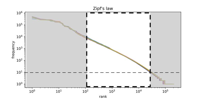
Springer Nature 2021 LATEX template

4 Linguistic resources

language as the official language (by law or de facto)2 . Our corpora selected
these regions, see Table 1; we also considered five additional regions (US, CA,
GB, FR, and BR) with well-known migration, business, and tourism activities
of Spanish speakers. The number of Twitter users varies with each country;
since each country has different social, political, security, health, and economic
conditions, so we will try to avoid any generalization.
 As already mentioned, we collected publicly published tweets from 2016 to
2019 using the Twitter stream API. We limited our collection to geotagged
messages marked by Twitter as written in Spanish. We decided to let out of
the corpus messages from the year 2020 and posteriors to avoid disturbances in
social media regarding the COVID-19 pandemic since our objective is to build
a dataset and resources based on the language itself and not on the pandemic
event. Our strategy to collect tweets was to ask the API to accept messages
with at least one Spanish stopword,3 and are also being labeled as written in
Spanish by Twitter, i.e., keyword lang=es in Twitter API.4 After this filtering
procedure, we retain close to 800 million messages.
 To ensure a minimum amount of information in each tweet, we discard
those tweets with less than five tokens, i.e., words, emojis, or punctuation
symbols. We also removed all retweets to avoid duplication of messages and
reduce foreign messages commented by Spanish speakers.
 Table 1 shows statistics about our corpora describing aspects such as coun-
try, number of users, number of tweets, and number of tokens. The table shows
that Spain, the USA, Mexico, and Argentina are countries with more users.
Furthermore, they are also those with more tweets in the Spanish language,
but the USA falls considerably in this aspect. A similar proportion is observed
in the number of tokens column. Although, Argentina is the country with the
highest number of tokens, above Mexico and Spain, significantly.
 The table also lists the coefficients for the expressions behind Heaps’ law
and Zipf’s law; these are two well-known laws describing how the vocabu-
lary grows in text collections written in non-severe-agglutinated languages.
These both are properties of a corpus in a particular language. Heaps’ law nα
describes the sub-linear growth of the vocabulary on a growing collection of
size n. Zipf’s law represents a power-law distribution where a few terms have
very high frequencies, and many words occur with a shallow frequency in the
collection. The expression that describes Zipf’s law is 1/rβ , where r is the rank
of the term’s frequency.
 Figure 1a illustrates the Heaps’ law in a small sample of regions of interest.
One can observe its predicted sub-linearity and that Mexico has the lowest
growth in its vocabulary size according to the number of tokens. On the con-
trary, the US corpus shows faster vocabulary growth, possibly explained due
to the mix of languages in many messages.

 2
 https://en.wikipedia.org/wiki/List_of_countries_where_Spanish_is_an_official_language
 3
 Words that are so common in a language that many NLP modeling schemes removed them in
many NLP. These words are articles, prepositions, interjections, and auxiliary verbs, among other
typical words. We use a stopword list with 400 common words to follow API’s limits.
 4
 Please note that any misclassification of language made by Twitter is conserved.
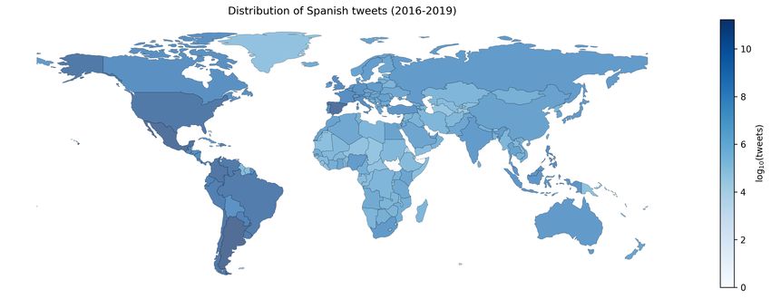
Springer Nature 2021 LATEX template

 Linguistic resources 5

Table 1: Statistics of our datasets after filtering by retweets and ensuring at
least five words per tweet. We show the origin country, the country code in ISO
3166-1 alpha-2 format as reported by the Twitter API, the number of tweets,
and the number of different users in the collected period.
 country code α β number of number of number of
 users tweets tokens

 Argentina AR 0.7563 1.8594 1,376K 234.22M 2,887.92M
 Bolivia BO 0.7509 1.8913 36K 1.15M 20.99M
 Chile CL 0.7555 1.8874 415K 45.29M 719.24M
 Colombia CO 0.7562 1.8993 701K 61.54M 918.51M
 Costa Rica CR 0.7447 1.8595 79K 7.51M 101.67M
 Cuba CU 0.7640 1.8677 32K 0.37M 6.30M
 Dominican Republic DO 0.7544 1.8832 112K 7.65M 122.06M
 Ecuador EC 0.7538 1.8968 207K 13.76M 226.03M
 El Salvador SV 0.7494 1.9066 49K 2.71M 44.46M
 Equatorial Guinea GQ - - 1K 8.93K 0.14M
 Guatemala GT 0.7498 1.9175 74K 5.22M 75.79M
 Honduras HN 0.7486 1.8941 35K 2.14M 31.26M
 Mexico MX 0.7557 1.8895 1,517K 115.53M 1,635.69M
 Nicaragua NI 0.7445 1.8535 35K 3.34M 42.47M
 Panama PA 0.7559 1.8952 83K 6.62M 108.74M
 Paraguay PY 0.7511 1.8815 106K 10.28M 141.75M
 Peru PE 0.7583 1.8966 271K 15.38M 241.60M
 Puerto Rico PR 0.7498 1.8433 18K 0.58M 7.64M
 Spain ES 0.7648 1.9036 1,278K 121.42M 1,908.07M
 Uruguay UY 0.7516 1.8346 157K 30.83M 351.81M
 Venezuela VE 0.7614 1.8959 421K 35.48M 556.12M

 Brazil BR 0.7681 1.9389 1,604K 27.20M 142.22M
 Canada CA 0.7652 1.9331 149K 1.55M 21.58M
 France FR 0.9372 1.9324 292K 2.43M 27.73M
 Great Britain GB 0.7687 1.9129 380K 2.68M 34.62M
 United States of US 0.7666 1.8929 2,652K 40.83M 501.86M
 America

 Total 12M 795.74M 10,876.25M

 Figure 1b shows the Zipf’s law under a log-log scale and, therefore, its quasi-
linear shape. We can see slight differences among curves, more noticeable on
both the left and right parts of the plot. The left part of the curves corresponds
to those terms with very high frequency, and the right side is dedicated to
those terms being rare in the collection. Notice that all these curves are similar
but slightly different; this is not a surprise since we analyze different dialects
of the same idiom, i.e., the Spanish language.

2.1 Geographic distribution
Figure 2a illustrates the number of collected Spanish language tweets over the
world. The color intensity is on a logarithmic scale, which means that slight
variations in the color imply significant changes in the number of messages;
countries with the darkest blue have the highest number of tweets in Spanish.
This figure shows how American countries (in the south, central, and north)
have, as expected, more tweets in the Spanish language than the rest of the
world.
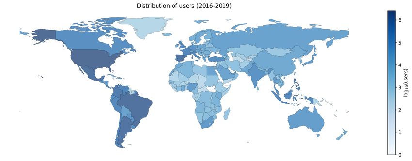
Springer Nature 2021 LATEX template

 6 Linguistic resources
 Heaps' law Zipf's law
 106
 AR AR
 175000 CL CL
 CO 105 CO
 150000 MX MX
 125000 PE 104 PE
vocabulary size

 ES ES

 frequency
 100000 VE 103 VE
 CA CA
 75000 US US
 102
 50000
 25000 101

 0 100
 0.0 0.2 0.4 0.6 0.8 100 101 102 103 104 105
 number of tokens 1e7 rank

 (a) Heaps law. Vocabulary size with (b) Zipf’s law. Frequency of tokens.
 respect to the number of tokens.

 Fig. 1: The vocabulary growth and distribution of frequencies of 107 tokens
 over a sample of our Twitter’s Spanish language corpora.

 Figure 2b shows the distribution of tweeters (users) per country. As in the
 previous image, we present a logarithmic scale in the intensity of color to rep-
 resent the number of users. The differences between this figure and Figure 2a
 are low, as expected, and follow the same distribution. Note the high intensity
 of American countries.

 (a) Distribution of tweets tagged as Span- (b) Distribution of the number of tweeters
 ish by Twitter. with at least one tweet tagged as Spanish
 language.

 Fig. 2: Distribution of tweets and tweeters labeled as Spanish-speaking users
 around the world. Colors are related to the logarithmic frequencies in data
 collected from 2016 to 2019 with the public Twitter API stream. Darker colors
 indicate a high population; the logarithmic scale implies that only significant
 frequency differences produce color changes.

 3 Lexical resources application
 This section describes and analyzes our Spanish Twitter Corpora (TSC) in the
 lexical aspect, specifically from the vocabulary usage perspective. This analysis
 complements that given of the Heaps’ and Zipf’s laws and the information
 given in Table 1.
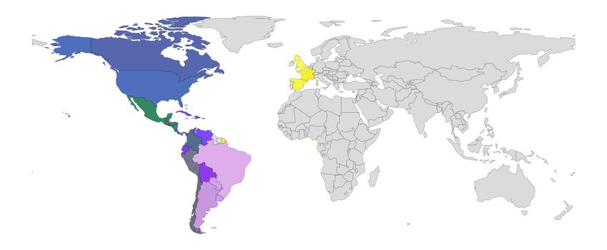
Springer Nature 2021 LATEX template

 Linguistic resources 7

 Figure 3 describes the procedure applied to obtain an affinity matrix of
our Spanish corpora. For this purpose, we extracted the vocabulary of each
corpus, i.e., a matrix that describes the similarities among corpora. The vocab-
ulary was computed on the entire corpus after text normalizations described
in the diagram. We also count the frequencies of all terms to obtain a Zipf-
like representation. We removed the one hundred more frequent words; we
also removed those terms with less than ten occurrences in the corpus from
the corpus vocabulary. Therefore, we kept the portion of the vocabulary that
illustrates the figure. The remaining terms and frequencies are used to create
a vector that represents the regional corpus.
 The affinity matrix is then computed using the cosine distance described
in the flow diagram. The heatmap represents the actual values in the matrix.
This matrix is crucial for the rest of this analysis since it contains distances
(dissimilarities) among all pairs of our Spanish corpora. Values close to zero
(darker colors) imply that those regions are pretty similar, and lighter ones
(close to one) are those regions with higher differences in their vocabularies. For
instance, the affinity matrix can show us how Mexico (MX) is more similar to
Honduras (HN), Nicaragua (NI), Peru (PE), and the USA (US). This behavior
could be the geographical location of the countries, and therefore, a large
migration or cultural interchange is made. On the other hand, Brazil (BR)
and Equatorial Guinea (GQ) are among the most atypical countries with low
similarities with the other countries.
 Figure 4 illustrates the similarity between Twitter country vocabularies.
We applied UMAP projections (2d for spatial projection and 3d for colorizing
points) using the affinity matrix as input. The figure shows how close or far are
each Spanish variation among the entire corpora. UMAP is parameterized by
the number of nearest neighbors (knn) in the affinity matrix, and thus, it can
consider local and global structures, depending on the number of neighbors.
 The figure shows the projection using 3nn; we can see four well-defined
clusters here. For instance, Uruguay (UY) is very close to Argentina (AR)
in three figures, and this is the case in other countries, like Mexico (MX),
Colombia (CO), and the United States (US); or Venezuela (VE), and Ecuador
(EQ).
 While some of these clusters support the idea that geographical similari-
ties imply language similarities, there are notorious exceptions. Figure 5 shows
a colorized map (using the UMAP 3D projection as colors). While it is pos-
sible to observe similarities and divisions among North America, Central and
South America, and European countries, there are important differences like
Colombia (being a Sudamericana country, it has more similarities to Central
American language variants. Regarding our lexical features, Cuba and the
Dominican Republic are also pretty close to Venezuela, Bolivia, and Ecuador.
It is interesting to recall that these lexical similarities are present in Twitter
and may vary from other data sources; nonetheless, it could be helpful to know
these affinities since tasks begin inherently regional (i.e., humor detection,
opinion mining) can take advantage of this knowledge.
Springer Nature 2021 LATEX template

8 Linguistic resources

 Input: Regional Spanish corpora
 Preprocessing and tokenization
 – lower casing
 Each regional vocabulary V were computed from – diacritic marks were removed
 geolocated tweets to each region. We drop the top – group users, urls, and numbers
 100 most frequent terms and also drop terms with less – normalize repetitions (2 max.)
 than 10 occurrences. – normalize blanks
 – laughs were normalized to four letters
 – words, punctuation, and emojis are tokens
 We define a global vocabulary L, of size `, as the
 union of all vocabularies. We use L to convert each
 vocabulary into a high dimensional vector X. Each
 vector’s coordinate corresponds with a term, and its
 value is the frequency of that term in the region
 corpus.

 The distance between two region vocabularies X, Y is
 the cosine dissimilarity;
 P`
 Xi · Yi Vocabularies
 dcos (X, Y ) = 1 − qP i=1 qP w1 w2 · · · w`
 ` 2 ` 2
 X
 i=1 i i=1 Yi VAR = f1AR f2AR · · · f`AR
 VBO = f1BO f2BO · · · f`BO
 . ...
 ..

 Output: Affinity matrix of regional vocabularies.

 Fig. 3: Affinity matrix among Spanish regions’ vocabularies.

 The most frequent words used in the vectors that represent each corpus are
shown in the word cloud in Figure 6a. While this is an illustrative figure, it is
possible to observe what kind of terms are used. We observe numerous types
of words, like verbs, adverbs, adjectives, and nouns; for instance, terms such
as personas, mundo, mañana (people, world, tomorrow), and tiempo (time)
are among the most used terms in the collection. We removed the one hun-
dred most frequent terms in each vocabulary to magnify differences in the
comparison.
 In addition, emojis are graphical symbols that can express an emotion or
popular concepts. Hence, they are a lexical resource that can also imply an
emotional charge. Emojis were created to compensate for the lack of facial
expressions and other expressive ways of face-to-face conversations. Therefore,
emojis are popular on social networks like Twitter since they are concise and
friendly ways to communicate [4]. The use of emojis is also dependent on the
region, as illustrated in Figure 6. The figure shows the 32 most used emojis
in each country; skin tone markers were separated from composed emojis and
Springer Nature 2021 LATEX template

 Linguistic resources 9

Fig. 4: Spanish-language lexical similarity visualization among country’s
vocabularies through a two-dimensional UMAP projection using the Cosine
among vocabularies. The points were colorized using a 3d UMAP projec-
tion (normalized and interpreted as RGB). Both projections use three nearest
neighbors, which emphasizes local features.

 Fig. 5: Regional Vocabulary in RGB representation

counted in an aggregated way. Note that the most popular emojis have con-
sensus in almost all regions. In top rank, we found the laughing face, the in
love face, and the heart (love). Another symbol that deserves attention is the
color-skin mask, which marks emojis with a skin hue. Regarding frequencies,
lighter color-skin marks are more popular than darker ones; this information
could have different meanings. For example, users identified as white people, or
perhaps it is just tricky to select the proper one with Twitter clients. The real
reason behind this finding is beyond the scope of this manuscript but deserves
attention.
Springer Nature 2021 LATEX template

10 Linguistic resources

 CC 1 2 3 4 5 6 7 8 9 10 11 12 13 14 15 16 17 18 19 20 21 22 23 24 25 26 27 28 29 30 31 32
 AR ❤ ♥ ♀
 BO ❤
 CL ❤ ♂ ♀
 CO ❤ ♀
 CR ❤ ♀ ♂
 CU ❤ ♂ ☀ ♀
 DO ❤ ♀ ♂
 EC ❤ ♀
 SV ❤
 GQ ❤
 GT ❤ ♥
 HN ❤ ♀ ♂
 MX ❤ ♀ ♂
 NI ❤ ♀
 PA ❤ ♀ ♂
 PY ❤ ♀
 PE ❤ ♥ ♀
 PR ❤
 ES ❤ ♀
 UY ❤ ♀ ♂
 VE ❤ ♥
 BR ❤ ♥
 CA ❤ ♀ ♂
 FR ❤ ☀ ♀
 GB ❤ ♀ ♂
 US ❤ ♀ ♂

(a) Frequent tokens in Spanish messages (b) Most popular emojis per Spanish-
in Twitter. speaking country.

Fig. 6: Word clouds of frequent tokens (a) and most used emojis in Spanish
(b)

4 Semantic analysis and regional word
 embeddings
This section explores the semantics of the Spanish language corpora proposed.
Each region has particular uses of some terms, and this effect induces differ-
ences when people communicate using a global perspective of a language. We
created local word embeddings that may help improve language understand-
ing regionally. Word embeddings are vector representations of a vocabulary
that capture the semantics of words learning how words are used in a large
text corpus. The model learns a high dimensional vector for each piece of the
text (word or token) using a distributional hypothesis: words used in similar
contexts have similar semantics. Therefore, if two vectors are close, then both
are semantically related; the contrary also becomes true, two distant vectors
are different semantically. In summary, word embeddings have become a pop-
ular and effective way to capture semantics from a corpus [11]. There exist
several techniques to learn word embeddings, for instance Word2Vec [8], Fast-
Text [7], and Glove [9]. Our resources are FastText models since it has support
for out-of-vocabulary words, which are pretty common in social network data.
FastText is both a word representation generator and text classification tool.
It is an open-source library well-known for its broad language coverage.5 For
instance, Grave et al. [12] trained word embeddings for 157 languages using
Wikipedia (800 million tokens) and Common Crawl (70 billion tokens); these
models include support for the Spanish language. Nonetheless, there is a lack

 5
 https://fasttext.cc/
Springer Nature 2021 LATEX template

 Linguistic resources 11

of country-level language support to the best of our knowledge. Our resources
are the first broad effort on this matter, making it possible to take advantage
of regionalisms and Spanish dialects.
 We use our Twitter corpora, divided by country, and apply our preprocess-
ing step, described in Section 3, as input of the FastText algorithm. Before, we
filtered out several messages as follows: we removed messages with URLs with
less than seven tokens and those produced by applications that use a template
to write the tweet (e.g., Foursquare), and we also removed retweeted messages.
These decisions emphasize that messages contain useful textual information
and do not reference external data. These filters reduced our corpora in half
(close to 400 million messages).
 As commented, were created 26 word-embedding models, one per country,
and were learn 300 dimension vectors, which is almost a standard for pre-
trained embeddings. We used the default values for the rest of the hyper-
parameters of FastText. In addition, for comparing purposes, we use the entire
corpora as a single corpus to create global word embeddings; the latter is the
strategy of most pre-trained word embeddings. This embedding is used to show
that regional word embeddings perform differently for regionalized tasks6 .
 We defined a representation and a similarity measure that considers seman-
tics for the similarity analysis. While each country word embedding assigns
vectors for each token, not all tokens exist on every corpus. More importantly,
even when vectors are structurally similar (300-dimensions), they cannot be
measured directly since the learning procedure only ensures that vectors are
comparable inside the same word embedding. Therefore, to be able to mea-
sure the similarity between different countries’ word embeddings, the following
procedure was performed:
• Select a common set of tokens; each token appears in at least ten countries.
 This filtering reduces the vocabulary from close to 1.7 million tokens to close
 to 118 thousand tokens (vocsize).
• We created a k nearest neighbor graph for each country using the dense
 vectors of the word embeddings closed to the set of common tokens; we select
 k = 33 after probing a number of choices. This k value captures several
 similar tokens and remains specific enough to let out different tokens. The
 cosine distance on the dense vectors was used.
• Each language variant (country) is represented as a high-dimensional vector
 that uses k entries per vocabulary word, one per neighbor in the common
 token set. Each token is then represented by its k nearest neighbors using the
 distance measure as weight. Note that each word embedding is represented
 with a sparse high-dimensional dataset, i.e., vocsize2 possible entries and
 approximately 3.8 million non-zero components.
 The set of Spanish embeddings are compared with the cosine distance on
the sparse vectors, and this is how we produced the affinity matrix shown
in Figure 7a. As a side effect of the high-dimensionality representation, most

 6
 These 27 embeddings are available in https://ingeotec.github.io/regional-spanish-models/
Springer Nature 2021 LATEX template

12 Linguistic resources

(a) Affinity matrix of our semantic repre-(b) Two dimensional UMAP projection of
sentations. semantic representations.

Fig. 7: Semantic similarities of our Spanish regional word embeddings. Coun-
tries are specified in their two letter ISO code. On the left, an affinity matrix
where darker cells indicate higher similarities (small distances). On the right
a two dimensional UMAP porjection, near points indicate similarity.

embeddings are farthest than in the lexical approach; however, the resulting
vectors can be effectively distinguished. As in the previous affinity matrix,
darker colors represent a major similarity between the regionalized embeddings
and the contrary with lighter colors.
 Figure 7b shows a two-dimensional UMAP projection of our semantic rep-
resentation affinity matrix. The projection uses three nearest neighbors; please
recall that few neighbors capture local structures. The colors are computed by
3D reduction by applying the UMAP dimensional reduction to the same input;
the resulting components create an RGB color set using a simple translation
and scale procedure to compose values between 0 and 1. Both distances and
colors describe a few well-defined groups. Please note that our ALL model is
quite different from most points and pretty similar to those regions with exten-
sive collections. This effect is available in word embedding models constructed
on non-regional corpora; they learn semantic traits of most represented regions.

4.1 A regional task example: predicting emojis with
 Emoji-15
Here we present the Emoji-15 classification task that exemplifies the pertinence
of regional models on the text classification task. For this task, we selected
15 popular emojis, see Section 3, and select 2020’s January and February
tweet messages having at most one of these emojis, and also geotagged to
one of our objective Spanish-speaking countries. Following the same filtering
procedure and preprocessing used for the word embedding, we also masked
emoji’s occurrences and that emoji was used as a label for the classification
task. It was obtained a number of examples that were divided into a 50-50
holdout (proportion of label messages remain similar in train and test set); see
Springer Nature 2021 LATEX template

 Linguistic resources 13

Table 2 for more details. We removed four countries (BO, CU, GQ, and PR)
from this task due to the low number of retrieved messages. For instance, we
kept the statistics of Cuba in the table to show the lower limit cutting. The
idea is to solve all-region benchmarks with all-region models and quantify their
performance and the pertinence of local models on local tasks.

 emoji AR BR CA CL CO CR CU DO EC ES FR GB GT HN MX NI PA PE PY SV US UY VE
 3,749 275 158 1,263 4,760 425 26 458 745 2,640 53 95 666 708 10,160 736 827 739 684 278 2,536 446 359
 ❤ 18,454 1,775 124 2,911 6,237 821 41 348 1,123 8,394 153 255 653 609 9,508 491 880 968 1,800 219 3,216 1,478 784
 2,114 92 34 1,016 1,455 242 20 167 253 1,825 41 58 376 157 2,754 159 313 160 666 124 597 190 71
 6,785 433 80 2,995 2,486 159 33 369 886 7,061 64 105 197 159 4,175 52 388 577 761 222 1,281 1,248 530
 4,278 100 28 390 1,407 161 7 123 200 1,164 26 37 134 91 1,438 105 260 115 428 31 667 283 142
 798 26 8 301 300 42 3 56 83 776 4 18 48 48 549 17 58 115 92 53 192 85 120
 3,609 105 35 1,803 1,475 171 32 175 364 3,827 74 56 257 129 3,395 115 236 817 369 192 829 377 293
 1,184 70 30 827 986 132 44 280 238 1,017 23 23 123 163 2,011 151 293 248 377 78 608 167 110
 15,999 932 111 2,190 6,824 510 28 509 837 8000 107 136 491 514 8,711 341 1,010 999 1,996 268 2,232 1,194 686
 3,081 89 24 920 1,718 155 50 316 291 780 18 22 163 124 2,185 175 322 213 259 127 738 359 236
 5,935 211 70 1,764 1,482 98 29 119 347 10,785203 99 171 72 4,290 63 136 374 190 181 1,808 719 493
 2,777 136 60 1,098 1,412 150 5 110 291 1,320 12 25 158 52 2,428 59 155 227 250 90 769 301 252
 2,144 89 38 699 1,039 153 8 102 296 1,507 31 39 151 129 2,646 131 204 271 239 69 781 227 135
 13,873 436 125 1,967 4,461 581 25 604 787 3,935 157 135 388 364 6,752 321 1,057 979 1,832 200 2,799 939 530
 6,751 275 154 2,756 4,173 440 47 614 771 4,781 99 111 421 339 7,380 211 741 1,135 937 384 1,941 951 734

Table 2: Train distribution of the emoji-15 datasets. Since it is a 50-50 hold-
out partition, the test set follows a similar distribution. We removed countries
with a low number of examples.

 The train partition was used to create one model per country and one for
the entire set of messages (called ALL). Figure 8 illustrates the normalized
performance of all models vs. all test databases, and Table 3 shows the precise
accuracy scores. The heatmap shows the performances among all regions vs.
all models. We can observe how some regions are difficult to predict, like CA,
NI, PA, DO, or SV (rows with many dark cells), and others particularly easy,
like AR, CO, ES, or MX. From the point of view of the models, some models
are also competitive, like US, VE, or ALL. One can observe that most accuracy
scores are pretty low but far from a uniform distribution (15 classes). In the
table, one can see the position that the local model achieves in each country
benchmark (local rank column). Note that small local rank values indicate that
the local model is efficient for its corresponding benchmark; this is evidence
that regional and local models may improve models on tasks requiring regional
knowledge. The best five models for each country benchmark are also listed;
we can observe how many geographically near regions perform well in their
geographic neighborhoods. The average rank of the local model is 8.09 while
the median is 6.5; these values support the idea that local models are useful
on tasks where regional information can be used. The US appears in several
benchmarks as part of their top-5 (seventeen times to be precise); the large
Springer Nature 2021 LATEX template

14 Linguistic resources

Fig. 8: Unit normalized accuracy scores for all models (columns) predicting
all region benchmarks (rows).

and diverse population of people living in the US with Latin American roots
could be the cause of this effect.
 The best performing model for a benchmark will rank as 1, the second-
best as 2, and similarly for the rest. The average rank of a single model along
all benchmarks indicates how well this model generalizes. Table 4 shows the
performance of all models along with all benchmarks, as its average rank. We
can observe that some country models are outstanding, like the US model.
On the other hand, the ALL model is competitive; however, it is not the best
(global 6th regarding average rank). Please recall that the ALL model was
created by merging the entire corpora into a single corpus, which is the typical
construction. In this sense, it is remarkable that smaller models like the US or
CO (both using a vocabulary of 300k tokens) perform better than huge ones
(the ALL model contains close to 1.7 million tokens in its vocabulary).
 While these results apply to the regional task of predicting the most popular
emojis, the evidence points that local models are competitive options for tasks
that require local traits as emoji predictions (see Table 3). Even more, some
regional models perform better than large models, as shown in Table 4, which
is a very important aspect.
Springer Nature 2021 LATEX template

 Linguistic resources 15

 country min max local top-5
 code acc. acc. rank

 AR 0.478 0.490 3 UY,PY,AR,PE,CO
 BR 0.461 0.488 1 BR,ALL,DO,PY,CR
 CA 0.293 0.353 18 CL,ALL,CO,MX,US
 CL 0.426 0.449 1 CL,US,MX,AR,ES
 CO 0.425 0.437 2 US,CO,VE,EC,GT
 CR 0.369 0.388 9 US,VE,ALL,MX,CO
 DO 0.338 0.381 13 US,CO,VE,CL,ALL
 EC 0.380 0.414 9 MX,US,CL,ALL,CO
 ES 0.475 0.486 1 ES,AR,MX,US,VE
 FR 0.419 0.442 4 ALL,GT,EC,FR,PA
 GB 0.347 0.376 23 ALL,AR,ES,VE,MX
 GT 0.349 0.388 13 MX,US,ALL,CO,ES
 HN 0.335 0.367 18 PE,EC,BR,CR,UY
 MX 0.423 0.434 1 MX,GT,CR,US,CO
 NI 0.337 0.372 18 VE,CO,CL,MX,US
 PA 0.366 0.393 10 US,CL,VE,CO,PE
 PE 0.380 0.420 9 MX,ALL,US,AR,CO
 PY 0.424 0.442 1 PY,US,BR,PE,UY
 SV 0.323 0.395 18 US,CO,MX,CL,VE
 US 0.404 0.424 1 US,MX,CO,ES,CL
 UY 0.435 0.457 1 UY,US,CO,CL,VE
 VE 0.385 0.434 4 MX,CO,ES,VE,US

Table 3: Performance statistics of all benchmarks (countries). Top-5 models
are also listed and the rank position of the local model on solving the current
benchmark.
Springer Nature 2021 LATEX template

16 Linguistic resources

 model voc. avg.
 size rank

 US 292,465 4.23
 CO 324,635 6.05
 MX 438,136 6.27
 CL 282,737 6.91
 VE 271,924 7.00
 ALL 1,696,232 8.45
 PE 178,113 8.64
 UY 200,032 8.73
 EC 147,560 8.95
 AR 673,424 9.41
 ES 571,196 10.95
 PY 124,162 11.14
 BR 127,205 11.27
 CR 103,086 12.50
 PA 111,635 13.36
 GT 95,252 13.64
 DO 108,655 14.91
 GB 82,418 18.00
 NI 68,605 18.18
 FR 69,843 18.91
 CA 63,161 19.00
 SV 73,833 19.14
 HN 60,580 20.36

Table 4: Average rank of all regional models along all countries datasets.
Models with low average ranks are better.
Springer Nature 2021 LATEX template

 Linguistic resources 17

5 Language Models
Language Models (LM) are more sophisticated than word embeddings models
since they go beyond word semantics to context semantics and text genera-
tion. More detailed, methods like Word2Vec [8], FastText [7], and Glove [9]
generate fixed embeddings for each word independently if the word can take
different meanings depending on the context. For example, the word orange
can be a fruit or a color, depending on the context. Language Modeling is the
task of predicting the next word given some context, so they perform well in
distinguishing homonyms.
 In that sense, BERT [2] is an LM that has gained considerable attention
lately. It is a model that uses a series of encoders to generate embeddings
for each word depending on its context. What makes BERT different from
alternatives like ELMo [10] is that the same pre-trained model can be fine-
tuned for different tasks. The pre-train on BERT uses the Masked Language
Model (MLM) task where each input sentence was put a mask token on 15%
random words. Then, BERT was trained on a second task, the Next Sentence
Prediction (NSP) task, where the input has two sentences, with a separation
token in between, and the task was to predict if the second sentence followed
the first.
 Our resources include a regional pre-trained BERT model using the MLM
task over tweets for the countries AR, CL, CO, MX, ES, UY, VE, and the
US; i.e., larger ones. We also produce another language model over the entire
corpora. We applied the same preprocessing as the detailed in Section 3. All the
models had a series of two encoders with four attention heads each and output
512-dimensional embedding vectors. This configuration corresponds with the
small size model following the official BERT implementation setup. We chose
this setup based on the computational resources we had available. We name
our model BILMA, for Bert In Latin America. We used a learning rate of 10−5
with the Adam optimizer; CL, UY, VE, and the US were trained with three
epochs and AR, CO, MX, and ES for just one because of the size of their
corpus. All the trained models are available for download7 .
 Figure 9 shows the loss and accuracy of the MLM task during the training.
We can see that the BILMA model for AR was trained on double the number
of batches; that was because of the corpus size. The rest of the models were
trained on a similar number of batches.
 In Figure 10a we show the comparison of the models predicting the masked
words on all the regions over the test set of tweets. Some interesting points to
highlight are the following. First, the Argentina model got very high scores on
all the regions, even above their corresponding models for UY and CO. This
might be because this model was trained for like double the data. Second, some
models got better results in the ES region than theirs, like CL, CO, UY, VE,
and the US. The US region got the worst results for AR, CL, CO, ES, and UY
models. Finally, CO and UY were the models with lower accuracy.

 7
 https://ingeotec.github.io/regional-spanish-models/
Springer Nature 2021 LATEX template

18 Linguistic resources

 8 0.5
 AR
 7 CL
 CO 0.4
 6 MX
 ES
 5 UY 0.3

 Accuracy
 VE AR
 4
 Loss

 US CL
 3 0.2 CO
 MX
 2 ES
 0.1 UY
 1 VE
 US
 0 0.0
 0.0 0.2 0.4 0.6 0.8 1.0 0.0 0.2 0.4 0.6 0.8 1.0
 number of batches 1e6 number of batches 1e6

 (a) Loss functions during training. (b) Accuracy functions during training.

Fig. 9: Loss and accuracy during training on the Masked Language Model
task. The batch size is of 128 tweets.

 AR 0.442 0.385 0.364 0.383 0.379 0.382 0.371 0.379 AR 0.487 0.385 0.364 0.369 0.383 0.386 0.32 0.35

 CL 0.399 0.421 0.373 0.391 0.386 0.364 0.378 0.378 CL 0.397 0.432 0.369 0.402 0.387 0.343 0.331 0.36

 CO 0.395 0.381 0.379 0.391 0.378 0.355 0.377 0.381 CO 0.389 0.377 0.419 0.404 0.38 0.332 0.325 0.378

 MX 0.397 0.382 0.368 0.409 0.379 0.356 0.375 0.385 MX 0.362 0.361 0.376 0.431 0.364 0.305 0.301 0.371
Regions

 Regions

 ES 0.427 0.422 0.403 0.417 0.453 0.396 0.409 0.417 ES 0.409 0.367 0.385 0.396 0.474 0.34 0.332 0.371

 UY 0.419 0.382 0.364 0.381 0.378 0.379 0.366 0.37 UY 0.47 0.401 0.379 0.391 0.402 0.431 0.335 0.38

 VE 0.4 0.399 0.371 0.395 0.392 0.367 0.404 0.386 VE 0.404 0.375 0.385 0.395 0.387 0.345 0.385 0.363

 US 0.39 0.377 0.363 0.39 0.376 0.351 0.372 0.396 US 0.373 0.364 0.364 0.391 0.371 0.308 0.3 0.407
 AR

 CL

 CO

 MX

 ES

 UY

 VE

 US

 AR

 ES
 CL

 CO

 MX

 UY

 VE

 US

 Models Models

 (a) Accuracy on the MLM task. (b) Accuracy predicting the emoticon.

Fig. 10: Comparison of the accuracy of the trained models on all the regions
on MLM and emoticon prediction tasks.

5.1 BILMA’s performance on the Emoji-15 regional task
We applied our BILMA models to our Emoji-15 task, see Section 4.1. For this
matter, we fine-tuned the pre-trained language models to predict the emoticon
by adding two linear layers. We split the tweets in 90% train and 10% validation
and trained until the accuracy stalled. After that, we evaluated the test set;
the results are presented in Figure 10b. We can conclude that all the models
got better results in their corresponding regions from the results. The AR,
MX, and ES models got good results over all the regions; meanwhile, UY and
VE got low scores. The prediction scores are pretty similar to those found in
Springer Nature 2021 LATEX template

 Linguistic resources 19

Table 3, however, our regional FastText models slightly improves on our fine-
tuned BILMA models. Nonetheless, BILMA models learns how people writes
in different regions, as it is exemplified in the rest of this section.

5.2 Generating text with BILMA regional language
 models.
As a qualitative and exemplification exercise, we present how each region model
predicts the masked word for the same example phrase. In Table 5 we show
the predictions for the masked token on a set of selected sentences. The color
intensity indicates the confidence of the model to predict the word. The first
two examples are el/la [MASK] subio de precio (the [MASK] raised in price)8 ,
here we can see differences in how each region name their public transportation,
in AR they use bondi, colectivo, in CL metro, micro, bus, in MX uber and ES
metro, bus; we can also see the differences in how they called the cellphone
service, in CO and MX is celular and in ES is movil. The third example is me
gusta tomar [MASK] en la mañana (I like to drink [MASK] in the morning)9 ,
here we can note that in AR and UY people prefer to drink mates meanwhile
in MX, ES, VE, and the US drink coffee. The fourth phrase is vamos a comer
[MASK] (let us eat [MASK]) where we can see the differences in the cuisine
of the countries with dishes like asado, pizza, ñoquis, empanadas, milanesas,
sushi, tacos, oreja, hamburguesa, arepa, torta. The last sentence is estoy en la
ciudad de [MASK] (I am in [MASK] city). The results include a list of some of
the larger cities in each region. This exercise is a proof of concept to show that
the models of different regions can predict very different words, i.e., regional
information.

6 Conclusions
This manuscript proposes a set of regionalized resources for the Spanish lan-
guage using Twitter as the data source. We collected messages from Twitter
public streaming API from 2016 to 2019; messages used must be tagged as
being written in Spanish and geotagged to one of the 26 countries considered
using Spanish as one of their primary languages. This procedure yields to our
Twitter Spanish Corpora with this procedure.
 The vocabulary of each corpus was extracted, characterized, and compared
their similarity, defining a distance metric between them. We also produce
visualizations and provide access to these vocabularies and their statistics. A
sample of the corpora through an open-source repository is also provided.
 On the other hand resources, we created regional semantic models using
FastText, and also some visualizations of the semantic similarities among
regions were produced. We also create regional language models called BILMA,
based on the well-known BERT transformer architecture. We provide access to

 8
 the article el indicates the masked word should be singular and masculine, and for la it should
be singular feminine
 9
 tomar could mean to take or to drink
Springer Nature 2021 LATEX template

20 Linguistic resources
 el [MASK] subio de precio
 AR CL CO MX ES UY VE US
 dolar chofer que cel que video internet que
 bondi metro tiempo video movil que video video
 que 0 0 uber tiempo profe 0 juego
 0 que agua numero bus 0 precio q
 auto bus se celular dia horoscopo telefono 0
 video internet ano tuit metro tema que pueblo
 autoestima papa dia que coche nombre dolar arbitro
 colectivo mio man telefono agua pibe queso tipo
 tiempo precio mundo dinero cafe grupo pan no
 tren profe celular tiempo pelo amor tlf mundo
 la [MASK] subio de precio
 AR CL CO MX ES UY VE US
 foto wea gente foto gente foto gente gente
 que gente vida vida que vida plata que
 lluvia micro noche gasolina foto gente semana foto
 luna foto que cancion vida historia caja prensa
 musica mama ley gente noche profe foto policia
 caja luna historia noche camara abuela carne tipa
 gente mina semana ropa cara cancion vida camara
 camara senora lluvia app bateria que cola ley
 coca profe luna pagina musica vieja arepa cara
 heladera vieja musica morra semana madre pasta 0
 me gusta tomar [MASK] en la manana
 AR CL CO MX ES UY VE US
 mates desayuno fotos cafe cafe mates cafe cafe
 teres once cafe fotos algo mate fotos decisiones
 cafe cafe cerveza decisiones nota algo ron ropa
 helado agua agua agua decisiones agua clases clases
 sol clases peliculas alcohol cerveza cafe decisiones manana
 fernet sol decisiones cerveza cola sol hoy fotos
 mate almuerzo hoy clases sol vino anis sol
 birra cerveza ropa hoy todo alcohol cartas agua
 algo hoy frio tequila uno helado agua hoy
 birras helado musica comida alcohol cerveza 0 comida
 vamos a comer [MASK]
 AR CL CO MX ES UY VE US
 asado sushi mierda tacos mierda algo pizza _
 pizza todo jaja mucho ya pizza mierda hoy
 algo hoy ! jaja mas hoy manana conmigo
 helado mierda rico pizza esto jaja rico pizza
 noquis algo . 0 mucho helado hamburguesa manana
 pizzas pizza _ manana jaja oreja hoy todo
 hoy ! helado hoy hoy todo arepa mierda
 empanadas jaja pizza taquitos tio nada . bien
 facturas ctm hoy emo usr uno todo playa
 milanesas emo asi algo bien eso torta tacos
 estoy en la ciudad de [MASK]
 AR CL CO MX ES UY VE US
 mierda santiago bogota mexico madrid mierda venezuela _
 argentina vina colombia monterrey espana casa caracas mexico
 cordoba conce cali guadalajara verdad uruguay valencia dios
 rosario chile medellin puebla sevilla hoy merida miami
 mierdaa valparaiso barranquilla cancun barcelona historia barquisimeto hoy
 tucuman stgo dios veracruz mierda nuevo maracaibo casa
 hoy concepcion hoy mty hoy filosofia maracay vacaciones
 capital valpo antioquia merida valencia ingles margarita pr
 aca maipu cartagena cdmx futbol montevideo aragua disney
 sol chillan paz todos examenes clase carabobo mi

Table 5: Predictions of the masked words over different regions. The color
intensity indicates the probability of prediction.

our word embedding and language models and the necessary packages, which
are also open-sourced under the MIT license.
 Finally, some insights into the usefulness of regional-aware models using
a per-country emoji prediction task were given. The results support that the
use of local and regional models could surpass massive word embeddings and
language models created in an agglutinate way.
Springer Nature 2021 LATEX template

 Linguistic resources 21

A BILMA language model usage
In order to use our BILMA models, we need to download one first, we will also
need the vocabulary file.
 To clone the repository, download the model and install dependencies, in
a linux terminal just type the following commands:

git clone https://github.com/msubrayada/bilma
cd bilma
bash download-emoji15-bilma.sh
python3 -m pip install tensorflow==2.4

and now we have the python package and its dependencies, the model and
the vocabulary file (shared to all BILMA models). In particular, this example
downloads the MX model that was trained with one epoch on the MLM task
and fine-tuned on the Emoji-15 task for 13 epochs.
 We need to run a Python 3 console and load the BILMA model.

from bilma import bilma_model
vocab_file = "vocab_file_All.txt"
model_file = "bilma_small_MX_epoch-1_classification_epochs-13.h5"
model = bilma_model.load(model_file)
tokenizer = bilma_model.tokenizer(vocab_file=vocab_file,
 max_length=280)

this BILMA model has two outputs, the first with shape (bs, 280, 29025)
where bs is the batch size, 280 is the max length and 29025 is the size of
the vocabulary. This output is used to predict the masked words. The second
output has shape (bs, 15) which corresponds to the predicted emoji.
 The next step is tokenizing some messages as follows:

texts = [
 "Tenemos tres dias sin internet ni senal de celular en el pueblo.",
 "Incomunicados en el siglo XXI tampoco hay servicio de telefonia
 fija",
 "Vamos a comer unos tacos",
 "Los del banco no dejan de llamarme"
]
toks = tokenizer.tokenize(texts)

the prediction is made as follows:

p = model.predict(toks)

finally, the predicted emojis can be displayed with:

tokenizer.decode_emo(p[1])
Springer Nature 2021 LATEX template

22 Linguistic resources

this produces the output: , each emoji corresponds
to the most probable one for each message in texts.

References
 [1] Crampton, Jeremy W., Mark Graham, Ate Poorthuis, Taylor Shelton,
 Monica Stephens, Matthew W. Wilson, and Matthew Zook. 2013. Beyond
 the geotag: situating "big data" and leveraging the potential of the
 geoweb. Cartography and Geographic Information Science, 40(2):130–139.

 [2] Devlin, Jacob, Chang, Ming-Wei, Lee, Kenton and Toutanova, Kristina.
 2019 BERT: Pre-training of Deep Bidirectional Transformers for Lan-
 guage Understanding Proceedings of the 2019 Conference of the North
 American Chapter of the Association for Computational Linguistics:
 Human Language Technologies, Volume 1 (Long and Short Papers), pages
 4171–4186, Association for Computational Linguistics

 [3] Donoso, Gonzalo and David Sánchez. 2017. Dialectometric analysis of
 language variation in Twitter. In Proceedings of the Fourth Workshop
 on NLP for Similar Languages, Varieties and Dialects (VarDial), pages
 16–25, Association for Computational Linguistics, Valencia, Spain.

 [4] Dresner, Eli and Susan C Herring. 2010. Functions of the nonver-
 bal in cmc: Emoticons and illocutionary force. Communication theory,
 20(3):249–268.

 [5] Graham, Mark, Scott A Hale, and Devin Gaffney. 2014. Where in the
 world are you? geolocation and language identification in twitter. The
 Professional Geographer, 66(4):568–578.

 [6] Huang, Yuan, Diansheng Guo, Alice Kasakoff, and Jack Grieve. 2016.
 Understanding us regional linguistic variation with twitter data analysis.
 Computers, environment and urban systems, 59:244–255.

 [7] Joulin, Armand, Edouard Grave, Piotr Bojanowski, and Tomas Mikolov.
 2017. Bag of tricks for efficient text classification. In Proceedings of the
 15th Conference of the European Chapter of the Association for Compu-
 tational Linguistics: Volume 2, Short Papers, pages 427–431, Association
 for Computational Linguistics.

 [8] Mikolov, Tomas, Ilya Sutskever, Kai Chen, Greg Corrado, and Jeffrey
 Dean. 2013. Distributed representations of words and phrases and their
 compositionality. In Proceedings of the 26th International Conference
 on Neural Information Processing Systems - Volume 2, NIPS’13, pages
 3111–3119, Curran Associates Inc., USA.
Springer Nature 2021 LATEX template

 Linguistic resources 23

 [9] Pennington, Jeffrey, Richard Socher, and Christopher D Manning. 2014.
 Glove: Global vectors for word representation. In Proceedings of the
 2014 conference on empirical methods in natural language processing
 (EMNLP), pages 1532–1543.

[10] Peters, Matthew E. and Neumann, Mark and Iyyer, Mohit and Gardner,
 Matt and Clark, Christopher and Lee, Kenton and Zettlemoyer, Luke.
 2018 Deep Contextualized Word Representations Proceedings of the 2018
 Conference of the North American Chapter of the Association for Com-
 putational Linguistics: Human Language Technologies, Volume 1 (Long
 Papers), pages 2227–2237, Association for Computational Linguistics

[11] Yang, Xiao, Craig Macdonald, and Iadh Ounis. 2018. Using word embed-
 dings in twitter election classification. Information Retrieval Journal,
 21(2):183–207.

[12] Edouard Grave, Piotr Bojanowski, Prakhar Gupta, Armand Joulin, and
 Tomas Mikolov. 2018. Learning Word Vectors for 157 Languages. Pro-
 ceedings of the International Conference on Language Resources and
 Evaluation (LREC 2018)

[13] CKennedy, Brendan and Atari, Mohammad and Davani, Aida
 Mostafazadeh and Yeh, Leigh and Omrani, Ali and Kim, Yehsong and
 Coombs, Kris and Havaldar, Shreya and Portillo-Wightman, Gwenyth
 and Gonzalez, Elaine and others (2022). Introducing the Gab Hate Cor-
 pus: defining and applying hate-based rhetoric to social media posts at
 scale. Language Resources and Evaluation, Springer.

[14] Escudero-Mancebo, David and Corrales-Astorgano, Mario and
 Cardeñoso-Payo, Valentín and Aguilar, Lourdes and González-Ferreras,
 César and Martínez-Castilla, Pastora and Flores-Lucas, Valle. 2022.
 Prautocal corpus: A corpus for the study of down syndrome prosodic
 aspects Language Resources and Evaluation, Springer.

[15] Gruszczyński, Włodzimierz and Adamiec, Dorota and Bronikowska,
 Renata and Kieraś, Witold and Modrzejewski, Emanuel and Wieczorek,
 Aleksandra and Woliński, Marcin, 2022. The Electronic Corpus of 17th-
 and 18th-century Polish Texts Language Resources and Evaluation,
 Springer.
You can also read