UNCERTAINTY QUANTIFICATION TECHNIQUES FOR SPACE WEATHER MODELING: THERMOSPHERIC DENSITY APPLICATION
←
→
Page content transcription
If your browser does not render page correctly, please read the page content below
U NCERTAINTY Q UANTIFICATION T ECHNIQUES FOR S PACE
                                                W EATHER M ODELING : T HERMOSPHERIC D ENSITY
                                                                A PPLICATION

                                                            Richard J. Licata                                           Piyush M. Mehta
                                              Dept. of Mechanical and Aerospace Engineering               Dept. of Mechanical and Aerospace Engineering
arXiv:2201.02067v1 [cs.LG] 6 Jan 2022

                                                         West Virginia University                                    West Virginia University
                                                         Morgantown, WV 26505                                        Morgantown, WV 26505
                                                        rjlicata@mix.wvu.edu

                                                                                             January 7, 2022

                                                                                              A BSTRACT

                                                 Machine learning (ML) has been applied to space weather problems with increasing frequency in
                                                 recent years, driven by an influx of in-situ measurements and a desire to improve modeling and
                                                 forecasting capabilities throughout the field. Space weather originates from solar perturbations and
                                                 is comprised of the resulting complex variations they cause within the numerous systems between
                                                 the Sun and Earth. These systems are often tightly coupled and not well understood. This creates a
                                                 need for skillful models with knowledge about the confidence of their predictions. One example of
                                                 such a dynamical system highly impacted by space weather is the thermosphere, the neutral region
                                                 of Earth’s upper atmosphere. Our inability to forecast it has severe repercussions in the context of
                                                 satellite drag and computation of probability of collision between two space objects in low Earth
                                                 orbit (LEO) for decision making in space operations. Even with (assumed) perfect forecast of model
                                                 drivers, our incomplete knowledge of the system results in often inaccurate thermospheric neutral
                                                 mass density predictions. Continuing efforts are being made to improve model accuracy, but density
                                                 models rarely provide estimates of confidence in predictions. In this work, we propose two techniques
                                                 to develop nonlinear ML regression models to predict thermospheric density while providing robust
                                                 and reliable uncertainty estimates: Monte Carlo (MC) dropout and direct prediction of the probability
                                                 distribution, both using the negative logarithm of predictive density (NLPD) loss function. We show
                                                 the performance capabilities for models trained on both local and global datasets. We show that
                                                 the NLPD loss provides similar results for both techniques but the direct probability distribution
                                                 prediction method has a much lower computational cost. For the global model regressed on the
                                                 Space Environment Technologies High Accuracy Satellite Drag Model (HASDM) density database,
                                                 we achieve errors of approximately 11% on independent test data with well-calibrated uncertainty
                                                 estimates. Using an in-situ CHAllenging Minisatellite Payload (CHAMP) density dataset, models
                                                 developed using both techniques provide test error on the order of 13%. The CHAMP models – on
                                                 validation and test data – are within 2% of perfect calibration for the twenty prediction intervals tested.
                                                 We show that this model can also be used to obtain global density predictions with uncertainties at a
                                                 given epoch.

                                        1   Introduction

                                        Low Earth orbit (LEO) will see the addition of tens of thousands of satellites in the coming years as private companies
                                        are developing mega constellations for the new space economy [1]. This congestion of certain orbital regimes increases
                                        the likelihood of a future collision between two objects. Satellite collisions can create debris clouds consisting of
                                        thousands of objects large enough to pose significant threats to other space assets. The 2009 Iridium-Cosmos collision
                                        resulted in approximately 2,300 observable debris objects, 65% of which remained in orbit seven years later [2]. Debris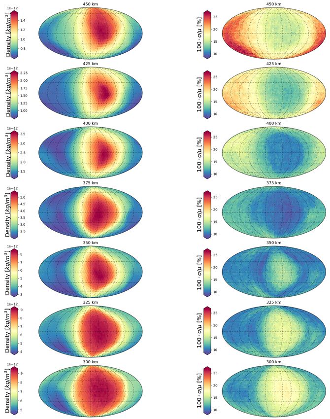
P REPRINT - JANUARY 7, 2022

objects created by collisions or weapons tests can catapult into highly elliptical orbits which pose a danger to satellites
in multiple orbital regimes [3].
In an effort to prevent these events from occurring, objects are continuously tracked, and their trajectories are predicted.
However, uncertainties play a large role in the prediction of future satellite positions. In LEO, atmospheric drag is the
largest single source of uncertainty mainly due to an incomplete understanding of the thermosphere. Variations in the
thermosphere are connected to temperature changes, as the atmosphere expands and contracts. Solar extreme ultraviolet
(EUV) and far ultraviolet (FUV) irradiance are the primary heating sources [4]. This absorption of solar irradiance
provides the baseline thermospheric mass density [5]. The effects of solar emissions are well-represented by various
solar indices and proxies [6].
Solar irradiance is generally a long-term variation while the solar wind drives more rapid changes in the thermosphere.
Mass and energy from the sun – manifested as the solar wind – travel through space and interact with the near-Earth
geospace environment. Certain events (e.g. coronal mass ejections) send massive amounts of energy and mass that
result in significant increases in thermospheric density. Energy, and therefore density, enhancements first appear in
the auroral zone (high latitudes) and propagate towards the equator in the form of traveling atmospheric disturbances
[7]. Geomagnetic storms are a particularly difficult phenomena to model and our current density models carry high
uncertainty during these periods [8, 9].
Satellite accelerometers have provided a unique insight into the thermosphere with high fidelity in-situ measurements,
particularly during storms [10]. Accelerations caused by non-drag sources (e.g. gravity and solar radiation pressure) are
modeled out allowing the isolation of drag acceleration that is then used to estimate mass density [11, 12, 13, 14, 15].
Drag acceleration is given as
                                                          1 cD A 2 vrel
                                                ~adrag = − ρ    v                                                          (1)
                                                          2 m rel |vrel |
where ~adrag is the drag acceleration, ρ is local mass density, cD is the satellite drag coefficient, A is the cross-sectional
area, m is the satellite mass, and vrel is the relative velocity of the satellite with respect to the rotating atmosphere. With
an estimate for drag acceleration, the density can be estimated, assuming adequate knowledge of the drag coefficient
and cross-sectional area given the satellite orientation. Density estimates obtained through this method are considered
ground truth and often used for model validation.
Accelerometer and orbit-derived densities have been used frequently in developing empirical models [16, 17, 18].
Furthermore, they have been used in data assimilation schemes to make corrections to background models, either
through observed orbital drag data [19] or two-line element data [20]. The most prominent integration of real-time
data for neutral density modeling is the High Accuracy Satellite Drag Model’s (HASDM) Dynamic Calibration of the
Atmosphere (DCA). This uses observed satellite data to make corrections to a background empirical density model [21].
Even with these improvements, density models have high errors, and we generally use them without any knowledge
of their confidence given the conditions. Until recently, no thermospheric density models – whether physics-based
or empirical– provided estimates of uncertainty. Bruinsma et al. (2021) developed an uncertainty-based version of
DTM2020 using polynomials to describe the 1-sigma uncertainties as a function of the inputs [22]. Licata et al. (2021)
used MC dropout to obtain uncertainty estimates for a global density modeling application with good calibration,
providing baseline performance [23]. In this work, we leverage ML to generate predictive density models for the
thermosphere that also provide robust and reliable uncertainty estimates. This is done for both a global and local
datasets using two methods: Monte Carlo (MC) dropout and a direct prediction of the probability distribution (referred
to primarily as direct probability).
We first outline the data and methods used for model development and analysis. Then, we use artificial data to
demonstrate the techniques. We move to the results for modeling with the global density dataset using the two
uncertainty techniques and perform a similar analysis for the models developed on local measurements. We also look at
the global prediction capabilities of the model developed with in-situ data, and we compare the evaluation times of both
uncertainty methods.

2     Datasets

2.1   SET HASDM Density Database

The High Accuracy Satellite Drag Model (HASDM) is the operational thermospheric density framework used by
the United States Space Force (USSF) [21]. By improving the density correction techniques presented by Marcos
et al. (1998) [24] and Nazerenko et al. (1998) [25], HASDM modifies 13 global temperature coefficients to make
real-time corrections to the Jacchia-Bowman 2008 Empirical Thermospheric Density Model (JB2008) [17]. Its Dynamic
Calibration of the Atmosphere (DCA) algorithm ingests data from calibration satellites that are distributed in altitude

                                                              2
P REPRINT - JANUARY 7, 2022

between 190 and 900 km – most are between 300 and 600 km [26]. As the algorithm provides corrections to JB2008,
HASDM provides global measurements on a 24×19×27 grid. For additional information on HASDM, the reader is
referred to Storz et al. (2005).
While HASDM is highly desired due to its real-time data assimilation, it is a proprietary model that is inaccessible to
researchers and operators. Space Environment Technologies (SET) is the contractor responsible for validating HASDM
outputs on a weekly basis, and they recently released HASDM validation archives from 2000-2020 covering close
to two full solar cycles providing good statistical coverage. This data release constitutes the SET HASDM density
database [27]. With a three-hour cadence, the database contains 58,440 global HASDM outputs. Each output has a
resolution of 15◦ longitude, 10◦ latitude, and 25 km altitude ranging from 175 to 825 km. For further details on the
SET HASDM density database and the validation process, the reader is referred to Tobiska et al. (2021).

2.2   Satellite Accelerometer Density Estimates

CHAllenging Minisatellite Payload (CHAMP) was launched in mid-2000 to study Earth’s gravity and magnetic fields
[28]. Its orbit is nearly polar with an inclination of 87.3◦ providing adequate global coverage, and it began at 460 km
in altitude. CHAMP was in orbit until 2010 when it stopped providing measurements at an altitude of approximately
300 km. The long mission lifetime covered nearly a solar cycle, providing measurements in solar maximum across
many strong geomagnetic storms and through the following solar minimum. Mehta et al. (2017) used higher fidelity
satellite geometry and improved gas-surface interaction models to scale the CHAMP density estimates of Sutton (2008)
[29, 30, 31, 32]. The density dataset starts on January 1, 2002 and ends on February 22, 2010 with a 10-second cadence.
The CHAMP dataset is prime for demonstration as spatiotemporally limited in-situ datasets are common in the space
weather field. This type of model can be built upon with the addition of density estimates from other satellites, displayed
in Figure 1.

Figure 1: Timeline of satellites with onboard accelerometers from 2000 – 2018 with bold lines representing the satellites’
mean altitude. Note: e-POP does not contain an accelerometer. The bottom panel shows the corresponding F10 values
indicating solar activity. The authors gratefully acknowledge Dr. Eelco Doornbos for providing this figure.

The addition of all satellites shown is Figure 1 would significantly expand the altitude coverage of the in-situ density
dataset. The CHAMP dataset used in this work has a 160 km altitude range and does not span a full solar cycle.
Integrating the density datasets of Gravity Recovery and Climate Experiment (GRACE) [33], Gravity Field and
Steady-State Ocean Circulation Explorer (GOCE) [34], and Swarm [35] would provide a thorough altitude coverage of
approximately 220 – 550 km and span from 2001 to present day. The Enhanced Polar Outflow Probe (e-POP) [36] is a
payload on Cascade, Smallsat and Ionospheric Polar Explorer (CASSIOPE) and its density estimates can be obtained

                                                            3
P REPRINT - JANUARY 7, 2022

through the processing of its Global Navigation Satellite System (GNSS) receivers [37, 38]. However, there is still
much active research related to the proper combination of different satellite density datasets [39, 40, 41]. Therefore, we
proceed with the standalone CHAMP dataset for demonstration.

2.3     Density Model Drivers

JB2008 uses four solar indices/proxies as drivers for solar activity. F10 – more completely referred to as F10.7 –
represents 10.7 cm solar radio flux and is a reliable proxy for solar EUV heating. S10 is an index for the integrated 26-34
nm solar EUV emission. The M10 proxy is a surrogate for FUV photospheric 160-nm Schumann-Runge Continuum
emissions. Y10 is a hybrid index that measures solar coronal X-ray emissions during solar maximum and Lyman-α
emissions during solar minimum. The S10 , M10 , and Y10 indices and proxies are not related to the 10.7 cm wavelength,
but they are converted to F10 units – solar flux units (sfu) – through linear regression. JB2008 also uses the 81-day
centered averages for all four solar drivers. This is indicated by the "81c" subscript. Additional information on these
solar drivers is provided by Tobiska et al. (2008).
To model geomagnetic activity, JB2008 uses a combination of ap and Dst. The ap index represents global geomagnetic
activity with a three-hour cadence. While it is widely used in density models, it is limited by the low-latitude range of
the measurements and its discrete range of 28 values. Dst is an index driven by the ring current strength in the inner
magnetosphere [42]. When Dstmin is below -75 nT, JB2008 shifts to using Dst as it improves storm-time performance
[17]. The EXTEMPLAR (EXospheric TEMperatures on a PoLyhedrAl gRid) model uses Poynting flux totals in the
northern and southern hemispheres – SN and SS , respectively [43]. Poynting flux represents electrodynamic energy
flowing into the upper atmosphere. The ap and Dst indices have 3-hour and 1-hour cadences, respectively. Therefore,
their use in a high-cadence model would not be advised. The geomagnetic index used to replace ap and Dst in the
CHAMP model is SYM-H, the longitudinally symmetric component of the magnetic field disturbances [44, 45]. SYM-H
is available with a 1-minute cadence.
The input sets for the HASDM and CHAMP models are shown in Table 1. The transformed time inputs t1 - t4 are defined
in Equation 2, and the transformed local solar time (LST) inputs are defined in Equation 3. These transformations are
performed to make the time and location inputs continuous.


                             2πdoy                           2πdoy                               2πU T                          2πU T
              t1 = sin                    ,   t2 = cos                    ,       t3 = sin                   ,   t4 = cos                   .   (2)
                             365.25                          365.25                                24                             24

                                                             2πLST                                     2πLST
                                          LST1 = sin                              LST2 = cos                                                    (3)
                                                               24                                        24

                                                Table 1: List of inputs for both models.
                                 HASDM                                                                     CHAMP
          Solar                Geomagnetic                    Temporal               Solar             Geomagnetic Spatial/Temporal
         F10 , S10 ,            apA , ap , ap3 ,                t1 , t2 ,           F10 , S10 ,          SYM-H,      LST1 , LST2 ,
        M10 , Y10 ,         ap6 , ap9 , ap12−33 ,               t3 , t4            M10 , Y10 ,           SN , SS     LAT , ALT ,
        F81c , S81c ,      ap36−57 , DstA , Dst,                                   F81c , S81c ,                         t1 , t2 ,
        M81c , Y81c         Dst3 , Dst6 , Dst9 ,                                   M81c , Y81c                           t3 , t4
                        Dst12 , Dst15 , Dst18 , Dst21

In Table 1, LST, LAT, and ALT are the local time, latitude, and altitude of the satellite, respectively. The "A" subscript
for the geomagnetic indices refers to the daily average. The numerical subscripts for these indices refer to the value that
many hours prior to prediction epoch. The combination of numbers refers to the average of that index over that many
hours prior to epoch. The HASDM input set originates from Licata et al. (2021) [46].

3     Methodology

3.1     Machine Learning

3.1.1     Principal Component Analysis
Principal Component Analysis (PCA), also referred to as Empirical Orthogonal Function (EOF) analysis, has been
widely used in thermospheric mass density applications. It has been applied to satellite accelerometer datasets (as

                                                                              4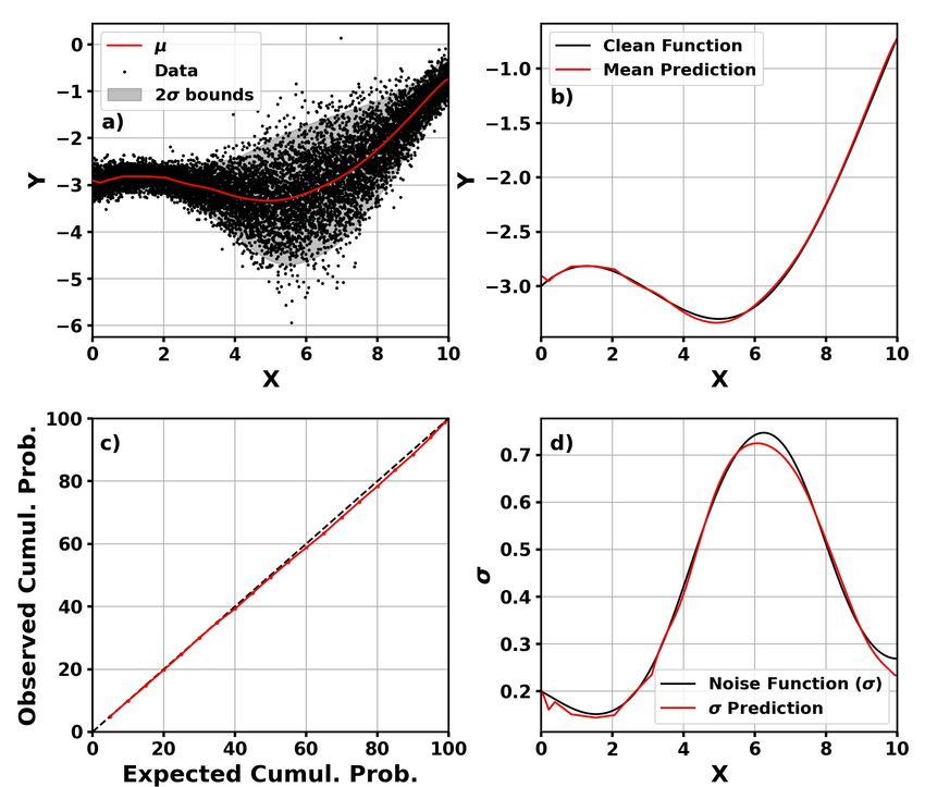
P REPRINT - JANUARY 7, 2022
described in Section 2.2) to identify dominant modes of variability in the thermosphere [47, 48, 15]. PCA is also used
in the field for dimensionality reduction as part of a reduced-order model (ROM) [49, 50, 51]. The HASDM dataset has
12,312 model outputs each epoch which makes uncertainty quantification (UQ) infeasible. Therefore, we apply PCA
to the dataset for ROM development with the goal of UQ. PCA is an eigendecomposition technique that maximizes
variance, determining uncorrelated linear combinations of data [52, 53]. We first take the common logarithm (log10 ) of
the density values to reduce the data’s variance then remove the spatial mean. PCA decomposes the data, separating the
spatial and temporal variations such that
r
X
x (s, t) = x̄ (s) + x
e (s, t) and x
e (s, t) = αi (t) Ui (s) (4)
i=1
In Equation 4, x (s, t) is the log density from HASDM, x̄ is the spatial mean, and xe is the variation about the mean.
αi (t) are temporal PCA coefficients and Ui are orthogonal modes – also called basis functions. The orthogonal modes
are derived through
X = U ΣV T where X = x x x ... x (5)
e1 e2 e3 em
U consists of orthogonal vectors representing the modes of variability. The Σ matrix contains the squares of the
eigenvalues – corresponding to the columns in U – along the diagonal. The data is encoded by performing matrix
multiplication with U.
3.1.2 Neural Network Modeling
In this work, we leverage neural networks (NNs) for nonlinear regression modeling due to their applicability as universal
function approximators and flexibility in development. A neural network is a collection of computational cells (or
neurons) connected in some form through multiplicative connections (or weights). Neural networks were first conceived
by McCulloch and Pitts (1943) when they described a computational representation of brain neurons and synapses with
calculus and statistical theory [54]. In the late 1950’s, the first artificial neural network (ANN) was developed and is
known as the perceptron [55]. Backpropagation is the process in which the network parameters are updated based on
observations and was fundamental to the development of modern neural networks [56, 57]. ANNs have been used
to directly predict thermospheric mass density using space weather indices and proxies as model drivers in order to
study long-term trends [58, 59]. These types of models can also be used as an exercise in understanding the effect
of the drivers on non-machine learning (ML) models [60]. Chen et al. (2014) [61] developed ANNs with different
combinations of geomagnetic indices to fit to CHAMP and GRACE density estimates during storms, and Choury et al.
(2013) [62] developed an ANN to predict exospheric temperature for use in the Drag Temperature Model (DTM).
3.1.2.1 Loss Functions
Loss functions are used to inform the NN of the objective during the training phase, or weight adjustment period. Loss
functions can be minimized or maximized depending on the modeling objective. A common loss function in regression
modeling is mean square error (MSE) given as,
n
1X 2
M SE(y, ŷ) = (yi − ŷi ) (6)
n i=1
where y is the ground truth, ŷ is the model prediction, and n is the batch size. The batch size is the number of samples
the model will pass through before updating the weights, averaging the loss over the batch. Losses are computed for
every output and backpropagation is how the model determines how much to change each weight. MSE is not used in
this work (explained in Section 3.1.2.2). We instead use the negative logarithm of predictive density (NLPD),
2
(y − µ) ln(σ 2 ) ln(2π) (7)
N LP D(y, µ, σ) = 2
+ +
2σ 2 2
where y is the observed value, µ is the predicted mean, and σ is the standard deviation of the output corresponding
to each unique input. NLPD is derived from −ln(f (x)) where ln is the natural logarithm and f (x) is the probability
density function of the normal distribution.
5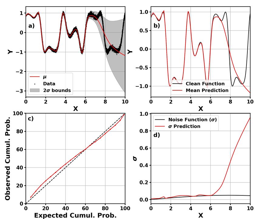
P REPRINT - JANUARY 7, 2022
3.1.2.2 Hyperparameter Optimization
Tools like Keras Tuner have drastically reduced model development time [63]. You can provide ranges of hyperpa-
rameters and Keras Tuner will explore the search space. We use the Bayesian optimization scheme, allowing the tuner
to perform a random search for the first 25 trials, or architectures, and using a Gaussian process model to choose the
architectures for the final 75 trails to exploit the high performing areas of the space. The objective of the tuner is to
minimize validation loss. The model optimizer and number of layers are first chosen by the tuner. For each layer, the
model can have a unique number of neurons, activation function, and dropout rate. For each model developed (two
datasets and two UQ techniques), the architecture is selected using Keras Tuner.
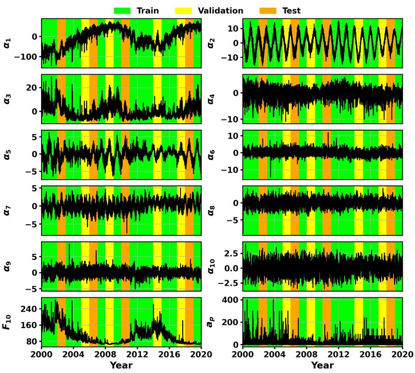
The 58,440 samples in the HASDM dataset are split into 60% training, 20% validation, and 20% test data. This is
displayed in Figure 2. As the number of training and validation samples is manageable, the full sets are used in tuning.
We obtain the HASDM models directly from the tuner without a need to train further.
Figure 2: First 10 HASDM PCA coefficients with F10 and ap . The shading represents the training, validation, and test
sets.
The CHAMP dataset is significantly larger with over 25 million total samples. Unlike the HASDM dataset, location is
now an input. CHAMP only covers the local solar time domain once every three months. The dataset also does not span
an entire solar cycle. Therefore, we repeat the following data split scheme. Eight weeks are used for training (483,840
samples), then the following week is used for validation (60,480 samples), and the next week is used for the test set
(60,480 samples). This results in similar input and output distributions while keeping temporally disjoint sets as there
are two weeks or 120,960 samples between the training segments. For the tuner, 1 million random samples are chosen
6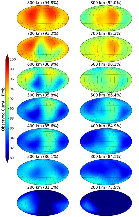
P REPRINT - JANUARY 7, 2022

from the training data and 500,000 random samples are chosen from the validation data. Once the tuner is complete, the
best models are retrained on the full training set and evaluated on the other two sets.

3.2     Uncertainty Quantification

A common method for uncertainty quantification is the use of Gaussian process (GP) models. GP regression models
are a supervised learning technique that can provide predictions with probability estimates in both regression and
classification tasks [64]. A GP model essentially provides a distribution of functions that fit the data which allows us to
obtain a mean and variance for any prediction [65]. GP regression has been used recently in space weather applications
in both driver forecasting [66] and empirical model calibration [67]. Some limitations for GP implementations are
difficult interpretation of results for multivariate problems and computational cost with large datasets [68]. The size
of these datasets, particularly CHAMP, inhibits the use of GP modeling. Ensemble modeling – the combination of
predictions from multiple models – is another common approach to obtain uncertainty estimates [69]. Limitations to
ensemble methods include increased computational complexity and difficult optimization [70, 71]. We instead use two
ML techniques: MC dropout (Section 3.2.1) and direct probability distribution prediction (Section 3.2.2), as UQ with
machine-learned models is fairly unexplored in the space weather domain. Dropout is a generalization technique that
applies Bernoulli distributions in each layer to change the flow of information through the model [72, 73]. Dropout is
traditionally only active during training to maintain a deterministic form in prediction. By forcing dropout to remain
active in prediction, the model becomes probabilistic. MC dropout has been shown to be an approximation of a GP [74].
For both methods, we use the negative logarithm of predictive density (NLPD) loss function (Equation 7 in Section
3.1.2.1). Licata et al. (2021) found that the mean square error loss function resulted in underestimated uncertainty
estimates in surrogate modeling for the HASDM dataset [46].

3.2.1    Monte Carlo Dropout Implementation
The typical input and output shape is n × ninp and n × nout , respectively. n is the number of samples, ninp is the number
of inputs, and nout is the number of outputs. In training, the mean and standard deviation need to be unique to each
input sample, so the model has to be provided each input k times. k needs to be a large enough number to allow for
adequate representation of the predicted distribution. The inputs and outputs for training are stacked about a repeated
intermediary axis. The training samples are identical about k, but are unique about n. The new input and output shapes –
necessary for proper training – are n × k × ninp and n × k × nout , respectively. In each training batch, the mean and
standard deviation are taken with respect to the intermediate axis, and the NLPD loss can be computed.

3.2.2    Direct Probability Distribution Prediction
Another way to represent uncertainty is to directly predict the mean and standard deviation. The mean square error
loss function cannot be used here as there are no labels for the standard deviation. However, Nix and Weigend (1994)
used a neural network to directly predict the mean and variance of a toy dataset using the NLPD loss function [75]. We
implement this technique for the datasets presented. To accomplish this, we create a custom output layer with 2nout
neurons. The first nout neurons represent the mean prediction and have a linear activation function. The last nout neurons
represent the standard deviation and use the softplus activation function. The softplus function and its derivative – the
sigmoid function – are shown in Equation 8.
                                                                                  ex
                                       f (x) = ln(1 + ex )          f 0 (x) =                                            (8)
                                                                                1 + ex
The desired qualities of the standard deviation output are: (1) always positive and (2) having no upper bound. The
initial choice was the absolute value function. However, the resulting models had erratic loss values, and it was difficult
to obtain a good model. The softplus function is (1) always positive, (2) has no upper bound, (3) is monotonically
increasing, and (4) is differentiable across all inputs. This resulted in stable training losses and better models.

3.2.3    Metrics
To compare the predictive capability of the models developed, we look at the mean absolute error across the training,
validation, and test sets. The errors across different space weather conditions will be investigated as well. We also test
the reliability of the uncertainty estimates both qualitatively and quantitatively. The calibration error score is given as
                                                               nout X
                                                                    m
                                                       100% X
                                Calibration Error =                    p(zi,j ) − p(ẑi,j )                              (9)
                                                      m · nout i=1 j=1

where m is the number of prediction intervals (PIs) of interest. Here the PIs range from 5% to 95% with 5% increments
in addition to 99% – [0.05, 0.10, 0.15, ... , 0.90, 0.95, 0.99]. p(ẑi,j ) is the observed cumulative probability obtained by

                                                             7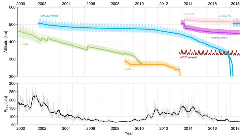
P REPRINT - JANUARY 7, 2022

dividing the number of true samples within the prediction interval by the total number of samples. Equation 9 is the
miscalibration of prediction intervals averaged over each output and prediction interval tested. For this work, it provides
the average deviation from all 20 PIs for each model output. We can visualize the reliability of the uncertainty estimates
by plotting the calibration curve – p(ẑ) vs p(z).

4   Toy Problems

To visualize the way the NLPD loss function influences training, we train models for two toy problems. Each problem
is a function, y(x), with additive Gaussian noise having zero-mean and a functional form to the standard deviation.
These functions are displayed in Table 2. The results for Problem 1 is shown in Figure 3

 Table 2: Functions for the two toy problems with the right column being the functional form of the Gaussian noise.
                                                      Function                         σ
                                                                                      sin(0.2x)
                                                                                    e
                          Problem 1      0.3x + cos(0.5x) − 4 + N (0, σ)       0.5
                                                                                  1+esin(0.8x)
                          Problem 2       sin (2x + cos(3x)) + N (0, σ)         0.05sin(0.2x)

Figure 3: Mean prediction with 2σ bounds plotted on data (a), clean function plotted with mean prediction (b),
calibration curve (c), and predicted standard deviation on true standard deviation function (d) for Problem 1.

Figure 3 shows that the model is able to adequately predict the function and is able to predict the overall probability
distribution. The interesting aspect of the figure is panel (d): the model is able to predict the standard deviation without

                                                             8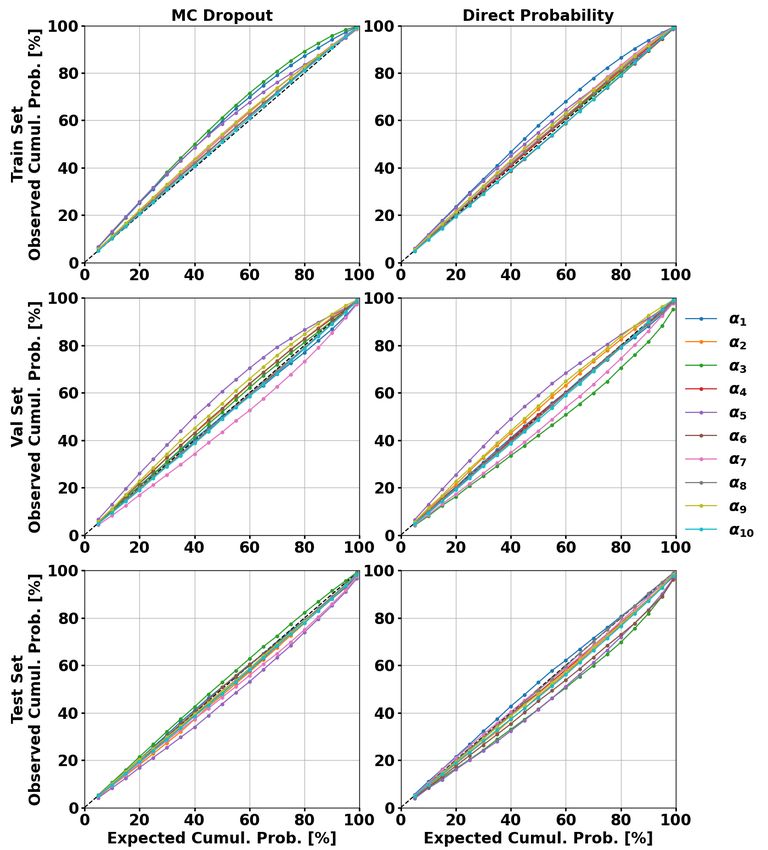
P REPRINT - JANUARY 7, 2022

a label. Meanwhile, this is fairly trivial data. Figure 4 shows the predictions and calibration curve for the more complex
Problem 2.

Figure 4: Mean prediction with 2σ bounds plotted on data (a), clean function plotted with mean prediction (b),
calibration curve (c), and predicted standard deviation on true standard deviation function (d) for Problem 2.

For the more complex data, the model is not as accurate over all x. When x < 6, the model can accurately predict the
mean and standard deviation. When x > 6, the standard deviation prediction no longer represents uncertainty in the data
but the model’s uncertainty in its prediction. For this portion of panel (b), the mean prediction deviates from the true
mean of the data and the standard deviation in panel (d) consequently increases. Panel (c) shows that the model is still
well-calibrated and representing both uncertainty in the data and uncertainty in the model’s predictions.
The NLPD loss function does not ensure model calibration. However, we show that it can be used – if properly tested
– in model development to represent uncertainty in the data and uncertainty in the model’s predictions. Note: these
models were trained on the entire dataset, and this is purely for demonstration. The thermospheric density models are
developed with separate validation and independent test sets.

5   HASDM Model

Using the best tuner models for MC dropout and direct probability distribution prediction, we assess the error and
calibration statistics. Table 3 shows the mean absolute error and calibration error score for both techniques across the
training, validation, and test sets.
It is evident that the performance using both methods is very similar. Across all three sets, the mean absolute error and
calibration error score do not deviate by more than 0.8% and 1.4% respectively. The MC dropout model has better

                                                            9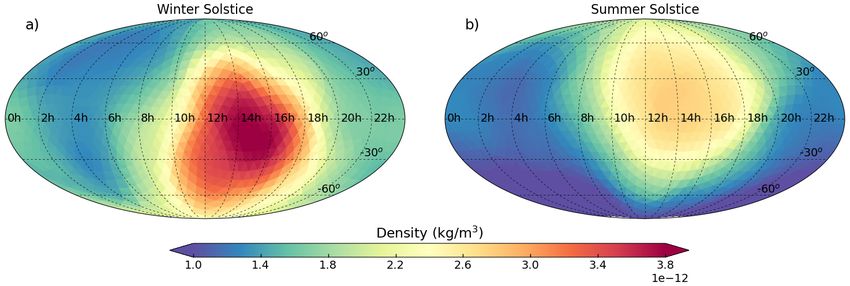
P REPRINT - JANUARY 7, 2022

Table 3: HASDM modeling results using MC dropout and direct probability prediction. Error refers to mean absolute
error, and calibration is computed using Equation 9.
                             Metric           Set         MC Dropout        Direct Probability
                                            Training        9.07%                 8.55%
                              Error        Validation      10.69%                 9.91%
                                              Test         10.69%                10.60%
                                            Training        3.06%                 1.74%
                           Calibration     Validation       2.51%                 2.45%
                                              Test          1.76%                 2.81%

performance on the independent test set in terms of calibration. This is a desired quality as the test data is not used
for model development in any way. As the calibration error scores are composites of the scores for each output, the
calibration curves are shown in Figure 5 for a qualitative assessment.
Both techniques lead to slightly overestimated uncertainties on the training set for multiple outputs. Meanwhile, the
remaining outputs are almost perfectly calibrated. On the validation set, each model has outputs with overestimated and
underestimated uncertainties. Again, most of the outputs are very well-calibrated which is affirmed by the calibration
error scores. For the test set, the direct probability prediction model tends to marginally underestimate the uncertainty
while the MC dropout model provides reliable uncertainty estimates on virtually all model outputs. Table 4 shows the
mean absolute error for both models across an array of solar and geomagnetic conditions. The entire dataset is used for
this analysis as there are not enough samples in each bin using only the test set.

     Table 4: Mean absolute error across global grid for HASDM-ML as a function of space weather conditions.
                                                    MC Dropout
                             F10 ≤ 75      75 < F10 ≤ 150 150 < F10 ≤ 190                F10 > 190       All F10
            ap ≤ 10           8.96%            9.78%                9.97%                  9.14%          9.50%
          10 < ap ≤ 50        9.76%            10.05%              10.87%                  9.90%         10.09%
            ap > 50           15.35%           12.86%              13.23%                 12.55%         13.01%
             All ap           9.12%            9.92%               10.36%                  9.55%          9.71%
                                                 Direct Probability
                             F10 ≤ 75      75 < F10 ≤ 150 150 < F10 ≤ 190                F10 > 190       All F10
            ap ≤ 10           8.64%            9.33%                9.35%                  9.11%          9.10%
          10 < ap ≤ 50        9.18%            9.51%                9.69%                  9.64%          9.48%
            ap > 50           11.14%           11.23%              11.34%                 10.30%         11.11%
             All ap           8.74%            9.42%                9.52%                  9.34%          9.23%

These errors tend to reiterate the results from Table 3. The direct probability model was more accurate on all three sets,
and Table 4 shows that it is also more accurate across all 20 conditions considered. For a majority of the conditions, the
difference is small (< 1%). However, the high ap conditions show that the direct probability model makes considerable
improvements. These error reduction from MC dropout range from 1.6 – 4.1%.
To further assess the uncertainty capabilities of the models, we attempt to visualize the calibration in the full-state
(global density grids) to identify any spatial dependence in the reliability of the uncertainty estimates. First, the models
are evaluated on the entire test set and the density mean and standard deviations are extracted. Using these statistics, the
observed cumulative probability with a 90% prediction interval is computed for each spatial location. The resulting
24 × 19 × 27 array is used to determine how well calibrated the model is on independent data as a function of location.
We show seven maps for each model (200, 300, ... , 800 km) in Figure 6. Even though HASDM has a lateral spatial
resolution of 24 longitude and 19 latitude segments, we interpolate the results to the polyhedral grid used in the
EXTEMPLAR model for visualization purposes. This is done in the remainder of the manuscript.
For reference, perfect calibration in Figure 6 would be uniform green maps at all altitudes. This would convey that with
a 90% prediction interval, the model’s predictions/uncertainty estimates contain 90% of true samples at all locations.
While this is not the case, the results are still insightful. At 200 km, both models are underestimating the uncertainty by
10 – 15%. This could be a result of the relative variability as a function of altitude in the SET HASDM density database.

                                                            10
P REPRINT - JANUARY 7, 2022
Figure 5: The left and right columns show the MC dropout and direct probability calibration curves, respectively. The
top, middle, and bottom rows are the calibration curves for the training, validation, and test sets, respectively.
The general trend of relative variability is that it increases with altitude, so the models may underpredict the standard
deviation at low altitudes as a result, which indicates that the model has a false sense of confidence in that region. Both
models have an average cumulative probability within 5% of the expected value at most of the altitudes shown in Figure
6 with the best results at 600 km. At 700 and 800 km, both models begin to overestimate uncertainty, likely because
they have the lowest confidence at those altitudes. An interesting outcome of this study is the lateral variability of the
cumulative probability between the models. The MC dropout model (left) has more lateral variability, meaning the
cumulative probability changes more as a function of longitude and latitude.
11P REPRINT - JANUARY 7, 2022
Figure 6: Observed cumulative probability maps for a 90% prediction interval using the MC dropout (left) and direct
probability (right) models. The average observed cumulative probability is shown for each altitude in parenthesis.
6 CHAMP Model
After running tuners for both uncertainty techniques, we trained the best models on the entire training set. The models
were chosen based on the lowest prediction error and best calibration scores on the validation set. Table 5 shows the
mean absolute error and calibration error scores on the three sets.
Both models are well-generalized in terms of prediction accuracy. The range in error between sets for the MC dropout
and direct probability model is 0.54% and 0.23%, respectively. Both models have higher calibration error scores on the
training set but have similar scores on the validation and test sets. The two techniques provide similar results with the
only notable difference is the 1.91% higher calibration error score for the direct probability model on the training set.
The calibration curves for both models are shown in Figure 7.
Both models are well-calibrated on all three sets. There is a tendency for both models to slightly overestimate uncertainty
on the training set which is more evident for the MC dropout model. The differences between the calibration curves and
the perfectly calibrated reference line (in black) is shown in panels (c) and (d). Panel (d) highlights the overestimation
of uncertainty for the direct probability model on the training set. However, it never deviates by more than 9%. Both
models tend to underestimate uncertainty on the validation and test set for the larger prediction intervals. Again, the
12P REPRINT - JANUARY 7, 2022
Table 5: CHAMP modeling results using MC dropout and direct probability prediction. Error refers to mean absolute
error, and calibration is computed using Equation 9.
Metric Set MC Dropout Direct Probability
Training 13.13% 12.59%
Error Validation 13.67% 12.82%
Test 13.14% 12.62%
Training 3.93% 5.84%
Calibration Validation 0.64% 0.25%
Test 0.22% 0.37%
Figure 7: Calibration curves for the training, validation, and test sets using MC dropout (a) and direct probability
prediction (b). Panels (c) and (d) show the difference between the observed and expected cumulative probability using
MC dropout and direct probability prediction, respectively.
deviation from perfect calibration is no more than 2% for any PI. Due to the intrinsic difference between the datasets
that the CHAMP and HASDM models are developed from, the proceeding analyses will be different than those in
Section 5.
6.1 Global Modeling with Local Measurements
The CHAMP models were developed with in-situ measurements, but we hypothesize that it should be able to learn
the functional relationship of the combined inputs. Therefore, the model should be able to provide global outputs at
any point in time. As a qualitative assessment, we show global maps at 400 km for the winter and summer solstices in
Figure 8 using the direct probability model. All proceeding global analyses will be performed using this model. For this
test, the solar drivers are all set to 120 sfu, SYM-H is set to 0 nT, both Poynting flux totals are set to 27GW, and the time
is set to 00:00 UTC.
The diurnal structure is present in both panels with the peak density being in the southern hemisphere during the winter
solstice and in the northern hemisphere during the summer solstice. This shows the model’s understanding on annual
trends (Earth’s tilt). The general density level is higher during the winter solstice, but the relative variation between day
and night are very similar. This is reaffirmed by the exospheric temperature distribution shown by Weimer et al (2020)
13P REPRINT - JANUARY 7, 2022
Figure 8: Global density map with moderate solar activity, low geomagnetic activity, the altitude fixed to 400 km, and
the time of day being 00:00 UTC for the winter solstice (a) and the summer solstice (b).
during the solstices. Additional global density maps at different altitudes can be found in Appendix A using baseline
conditions. Furthermore, a global storm example is shown in Appendix B.
Next, we look at the uncertainty levels for eight unique conditions of activity and time. These are all displayed in
Table 6. Using these space weather and temporal inputs, the CHAMP model is evaluated at all 1,620 polyhedral grid
locations from 300 to 450 km in 1 km increments. The metric we use here is a normalized measure of model uncertainty:
100 · σ/µ, essentially providing the 1-σ uncertainty as a percentage of the mean prediction. The resulting maps are
averaged across each altitude to evaluate the model’s uncertainty for each condition as a function of altitude. Three
aspects of model drivers are investigated: solar activity, geomagnetic activity, and temporal dependence. In Table 6,
there are three solar activity levels, with all other drivers kept constant. There are also three geomagnetic cases: low and
high geomagnetic activity with moderate solar activity, and high geomagnetic activity with high solar activity. We only
look at two daily cases – 00:00 and 12:00 UTC. We also look at the fall equinox, summer solstice, and winter solstice
with moderate solar and low geomagnetic activity. The resulting altitude profiles are shown in Figure 9.
Table 6: CHAMP model inputs to study various conditions as a function of altitude. * Solar 2 is also considered Geo 1,
UTC 1, and doy 1.
Solar Drivers Geomagnetic Drivers Temporal Drivers
Condition Name FMSY SYM-H SN = SS UTC doy
Solar 1 75 0 27 0 262
Solar 2* 120 0 27 0 262
Solar 3 190 0 27 0 262
Geo 2 120 -75 128 0 262
Geo 3 190 -75 128 0 262
UTC 2 120 0 27 12 262
doy 2 120 0 27 0 172
doy 3 120 0 27 0 355
Panel (a) in Figure 9 shows that the CHAMP model has low uncertainty in its lower altitude predictions for solar
minimum (or low solar activity) which drastically increases with altitude. The opposite can be said for solar maximum.
The moderate solar activity case results in lowest uncertainties between 350 and 375 km and higher uncertainties above
and below that range. This is all a result of CHAMP’s altitude from 2002-2010. It started around 460 km during solar
maximum and ended at 300 km during solar minimum. Therefore, the model has confident predictions in the altitude
range the satellite was located during the various phases of the solar cycle. If there was additional data from satellites at
different altitudes over a longer time period, the model would likely be more confident over a larger altitude range.
In panel (b), we see the same general trends for Geo 1 and Geo 2, because they are evaluated using moderate solar
activity. However, it is evident that the increase in geomagnetic activity results in up to 5% more uncertainty. The
Geo 3 case is similar to Solar 3 (high solar activity) but again has increased uncertainty due to the storm conditions
it represents. Panel (c) indicates that there is a low impact from universal time on the model uncertainty. In Panel
14P REPRINT - JANUARY 7, 2022
Figure 9: Normalized uncertainty variations as a function of altitude for solar (a), geomagnetic (b), daily (c), and annual
(d) cases. The drivers for each curve can be found in Table 6.
(d), the black line indicates the fall equinox which is similar to the winter solstice. The Winter solstice uncertainties
deviate from the equinox uncertainties at the highest altitude range. While the overall shape remains consistent, there
are highest uncertainties for the summer solstice at all altitudes. The overall takeaway form Figure 9 is that the shape
of the model uncertainty altitude profile is most strongly effected by the solar activity level while the day of year and
geomagnetic activity tend to uniformly increase or decrease uncertainty. These profiles would all likely be impacted if
the model was developed using additional satellite data.
7 Evaluation Time Comparison
We attempt to provide an equal comparison of the two methods in terms of computational complexity. To do so,
each CHAMP model is evaluated on either 8,640 samples (one week) or 86,400 samples (ten weeks). For the direct
probability prediction model, it sees each input once and provides the mean and standard deviation. These are used to
sample a Gaussian distribution 1,000 times to get probabilistic predictions for density over the given window.
For MC dropout, we cannot pass one week of inputs to the model stacked 1,000 times (as is done for HASDM). There
is not enough memory on an NVIDIA GeForce RTX 2080 Ti graphics processing unit (GPU) – 11 GB – to perform this
evaluation. Therefore, we pass the 100 repeated inputs in 10 chunks to obtain the 1,000 predictions. When evaluating
over ten weeks, we must reduce to 10 repeated inputs in 100 chunks. In Table 7, we show the evaluation times on both
GPU and CPU for both methods over the two durations. Note: when running MC dropout on CPU, we use 100 repeated
inputs for both durations. The batch size for all predictions is 217 or 131,072. The size of the MC dropout and direct
probability models are 233.3 kB and 21.9 MB, respectively.
The run times are unique to these specific models. The size of the models plays a role in run time, and the size of these
models are a result of the tuner. The MC dropout model is approximately 100 times smaller, but the increase in required
model prediction calls results in the significantly longer run times. The direct probability method, for this particular
problem, is anywhere from 3 to 30 times faster depending on the number of samples and whether the GPU or CPU is
being used.
15P REPRINT - JANUARY 7, 2022
Table 7: Run time to obtain 1,000 probabilistic predictions from each model using GPU and CPU in seconds.
Method Samples GPU Run Time CPU Run Time
8,640 2.11 13.65
MC Dropout
86,400 18.29 127.79
8,640 0.58 0.52
Direct Probability
86,400 3.93 3.93
8 Discussion and Conclusions
In this work, we leverage the NLPD loss function to develop thermospheric density models using 1) MC dropout
and 2) direct probability prediction. These two uncertainty techniques were used to create both a model based in the
PCA coefficients of the SET HASDM density database and a model based in localized accelerometer-derived density
estimates from CHAMP. Using two toy problems, we showed that the NLPD loss function can be used to create a ML
model with calibrated uncertainty estimates relative to uncertainty in the model, uncertainty in the data, or both. For the
HASDM database, the MC dropout and direct probability distribution prediction models had similar metrics in terms of
error and calibration. Furthermore, the calibration curves for the PCA coefficients were nearly identical. By looking at
the density calibration of both HASDM models, we found that they were well-calibrated at mid-altitudes, and there was
more lateral variability in the calibration of the MC dropout model.
The CHAMP models also had similar performance and were both well-generalized. We test the CHAMP model’s
global prediction capabilities by generating baseline maps during the winter and summer solstices to ensure physical
global trends are being captured by the CHAMP model. This showed that the model was able to emulate the effect of
Earth’s tilt. We also performed global evaluations for eight unique conditions to determine the altitude dependence
of model uncertainty. The altitude profiles showed that the minimum and maximum 1-σ uncertainties were 10 –
28% of the mean predictions, respectively. Solar activity was most influential in determining the profiles’ shapes
while geomagnetic activity and day of year tended to provide uniform changes in the uncertainty. In general, the MC
dropout and direct probability methods were shown to have similar performance for thermospheric density modeling
applications. However, there are pros and cons for both methods, and careful consideration is required when deciding
on a UQ method for space weather models. These are highlighted in Table 8.
Table 8: Pros and cons for MC dropout and direct probability distribution prediction.
Method Pros Cons
• No need to sample from a Gaussian • Longer evaluation times
MC Dropout
distribution • Not compatible with large datasets
• Only need single evaluation • Required sampling from a Gaussian distribution
Direct Probability
• Computationally efficient to obtain probabilistic predictions
The main disadvantage for the direct probability method is the requirement to sample from a Gaussian distribution to
get probabilistic density variations. The drawback to MC dropout is its higher computational cost. In terms of density
modeling, both techniques have prompt evaluation times. Relative to one another, we show that the direct probability
models can be evaluated much faster. The size of the training data (in both number of samples and dimensionality) is
also important to consider. With MC dropout, GPU memory can constrain modeling efforts if the dataset is too large. It
can also require additional steps for prediction. In this work, MC dropout did not inhibit model development for the
smaller HASDM PCA data. However, it did add numerous considerations when developing and evaluating the CHAMP
model. In general, the uncertainty estimation capabilities may be improved through modifications to the loss function to
either: a) add higher order moments or b) obtain non-Gaussian estimates.
All the preceding results show that for thermospheric density applications, these two techniques can be used to obtain
an accurate model with reliable uncertainty estimates. There are other methods that can be used in space weather
application such as GP regression and ensemble modeling, as previously mentioned, but this is a sufficient starting
point. Other final considerations concern orthogonality and applicability. For a multi output regression model (e.g.
HASDM models), the outputs must be orthogonal. This is to both prevent collinearity and since the use of NLPD
requires uncorrelated outputs. The CHAMP data only spans an altitude range of 300 – 460 km. Any predictions outside
of this range may be unreliable. To combat this, density estimates from other satellites can be added to increase the
altitude coverage and provide the model with more data to learn from, as discussed in Section 2.2.
16P REPRINT - JANUARY 7, 2022
Data Statement
Requests can be submitted for access to the SET HASDM density database at https://spacewx.com/hasdm/ and
all reasonable requests for scientific research will be accepted as explained in the rules of road document on the website.
The historical space weather indices used in this study can also be found at https://spacewx.com/jb2008/ in the
SOLFSMY.TXT, SOLRESAP.TXT, and DSTFILE.TXT files for the solar indices, ap, and Dst, respectively. Free
and one-time only registration is required to access these files. SYM-H data was obtained from http://wdc.kugi.
kyoto-u.ac.jp/aeasy/index.html thanks to the World Data Center for Geomagnetism in Kyoto. CHAMP density
estimates from Mehta et al. (2017) can be found at http://tinyurl.com/densitysets.
Acknowledgements
PMM gratefully acknowledges support under NSF CAREER award #2140204. The authors would like to acknowledge
DLR for their work on the CHAMP mission along with GFZ Potsdam for managing the data.
References
[1] J. Radtke, C. Kebschull, and E. Stoll, “Interactions of the space debris environment with mega constella-
tions—Using the example of the OneWeb constellation,” Acta Astronautica, vol. 131, pp. 55–68, 2017.
[2] C. Pardini and L. Anselmo, “Revisiting the collision risk with cataloged objects for the Iridium and COSMO-
SkyMed satellite constellations,” Acta Astronautica, vol. 134, pp. 23–32, 2017.
[3] A. C. Boley and M. Byers, “Satellite mega-constellations create risks in Low Earth Orbit, the atmosphere and on
Earth,” Scientific Reports, vol. 11, no. 1, 2021.
[4] R. G. Roble, Energetics of the Mesosphere and Thermosphere, pp. 1–21. American Geophysical Union (AGU),
1995.
[5] L. Qian and S. Solomon, “Thermospheric Density: An Overview of Temporal and Spatial Variations,” Space
Science Reviews - SPACE SCI REV, vol. 168, pp. 1–27, 06 2011.
[6] W. K. Tobiska, S. D. Bouwer, and B. R. Bowman, “The development of new solar indices for use in thermospheric
density modeling,” Journal of Atmospheric and Solar-Terrestrial Physics, vol. 70, no. 5, pp. 803–819, 2008.
[7] S. L. Bruinsma and J. M. Forbes, “Properties of traveling atmospheric disturbances (TADs) inferred from CHAMP
accelerometer observations,” Advances in Space Research, vol. 43, no. 3, pp. 369–376, 2009.
[8] D. M. Oliveira, E. Zesta, P. W. Schuck, and E. K. Sutton, “Thermosphere Global Time Response to Geomagnetic
Storms Caused by Coronal Mass Ejections,” Journal of Geophysical Research: Space Physics, vol. 122, no. 10,
pp. 10,762–10,782, 2017.
[9] S. Bruinsma, C. Boniface, E. K. Sutton, and M. Fedrizzi, “Thermosphere modeling capabilities assessment:
geomagnetic storms,” J. Space Weather Space Clim., vol. 11, p. 12, 2021.
[10] P. Ritter, H. Lühr, and E. Doornbos, “Substorm-related thermospheric density and wind disturbances derived from
CHAMP observations,” Annales Geophysicae, vol. 28, no. 6, pp. 1207–1220, 2010.
[11] S. Bruinsma and R. Biancale, “Total Densities Derived from Accelerometer Data,” Journal of Spacecraft and
Rockets, vol. 40, no. 2, pp. 230–236, 2003.
[12] H. Liu, H. Lühr, V. Henize, and W. Köhler, “Global distribution of the thermospheric total mass density derived
from CHAMP,” Journal of Geophysical Research: Space Physics, vol. 110, no. A4, 2005.
[13] E. K. Sutton, Effects of solar disturbances on the thermosphere densities and winds from CHAMP
and GRACE satellite accelerometer data. PhD thesis, University of Colorado at Boulder, Oct. 2008.
https://ui.adsabs.harvard.edu/abs/2008PhDT........87S.
[14] E. Doornbos, Producing Density and Crosswind Data from Satellite Dynamics Observations, pp. 91–126. Berlin,
Heidelberg: Springer Berlin Heidelberg, 2012.
[15] A. Calabia and S. Jin, “New modes and mechanisms of thermospheric mass density variations from GRACE
accelerometers,” Journal of Geophysical Research: Space Physics, vol. 121, no. 11, pp. 11,191–11,212, 2016.
[16] J. M. Picone, A. E. Hedin, D. P. Drob, and A. C. Aikin, “NRLMSISE-00 empirical model of the atmosphere:
Statistical comparisons and scientific issues,” Journal of Geophysical Research: Space Physics, vol. 107, no. A12,
pp. SIA 15–1–SIA 15–16, 2002.
17P REPRINT - JANUARY 7, 2022
[17] B. Bowman, W. K. Tobiska, F. Marcos, C. Huang, C. Lin, and W. Burke, “A New Empirical Thermospheric
Density Model JB2008 Using New Solar and Geomagnetic Indices,” in AIAA/AAS Astrodynamics Specialist
Conference, AIAA 2008-6438, 2008. https://arc.aiaa.org/doi/abs/10.2514/6.2008-6438.
[18] Bruinsma, Sean, “The DTM-2013 thermosphere model,” J. Space Weather Space Clim., vol. 5, p. A1, 2015.
[19] E. K. Sutton, S. B. Cable, C. S. Lin, L. Qian, and D. R. Weimer, “Thermospheric basis functions for improved
dynamic calibration of semi-empirical models,” Space Weather, vol. 10, no. 10, 2012.
[20] E. Doornbos, H. Klinkrad, and P. Visser, “Use of two-line element data for thermosphere neutral density model
calibration,” Advances in Space Research, vol. 41, no. 7, pp. 1115–1122, 2008.
[21] M. F. Storz, B. R. Bowman, M. J. I. Branson, S. J. Casali, and W. K. Tobiska, “High accuracy satellite drag model
(hasdm),” Advances in Space Research, vol. 36, no. 12, pp. 2497–2505, 2005.
[22] Boniface, Claude and Bruinsma, Sean, “Uncertainty quantification of the DTM2020 thermosphere model,” J.
Space Weather Space Clim., vol. 11, p. 53, 2021.
[23] R. J. Licata, P. M. Mehta, W. K. Tobiska, and S. Huzurbazar, “Machine-learned hasdm model with uncertainty
quantification,” 2021.
[24] F. Marcos, M. Kendra, J. Griffin, J. Bass, D. Larson, and J. J. Liu, “Precision Low Earth Orbit Determination
Using Atmospheric Density Calibration,” Journal of The Astronautical Sciences, vol. 46, pp. 395–409, 1998.
[25] A. Nazarenko, P. Cefola, and V. Yurasov, “Estimating atmospheric density variations to improve LEO orbit
prediction accuracy,” in AIAA/AAS Space Flight Mechanics Meeting, AAS 98-190, 1998. http://www.space-
flight.org/AAS_meetings/1998_winter/abstracts/98-190.html.
[26] B. Bowman and M. Storz, “High Accuracy Satellite Drag Model (HASDM) Re-
view,” in AIAA/AAS Astrodynamics Specialist Conference, AAS 03-625, 2003.
https://sol.spacenvironment.net/∼JB2008/pubs/JB2006_AAS_2003_625.pdf.
[27] W. K. Tobiska, B. R. Bowman, D. Bouwer, A. Cruz, K. Wahl, M. Pilinski, P. M. Mehta, and R. J. Licata, “The
SET HASDM density database,” Space Weather, p. e2020SW002682, 2021.
[28] C. Reigber, H. Lühr, and P. Schwintzer, “Champ mission status,” Advances in space research, vol. 30, no. 2,
pp. 129–134, 2002.
[29] P. M. Mehta, A. C. Walker, E. K. Sutton, and H. C. Godinez, “New density estimates derived using accelerometers
on board the CHAMP and GRACE satellites,” Space Weather, vol. 15, no. 4, pp. 558–576, 2017.
[30] P. M. Mehta, C. A. McLaughlin, and E. K. Sutton, “Drag coefficient modeling for grace using Direct Simulation
Monte Carlo,” Advances in Space Research, vol. 52, no. 12, pp. 2035–2051, 2013.
[31] P. M. Mehta, A. Walker, C. A. McLaughlin, and J. Koller, “Comparing Physical Drag Coefficients Computed
Using Different Gas–Surface Interaction Models,” Journal of Spacecraft and Rockets, vol. 51, no. 3, pp. 873–883,
2014.
[32] A. Walker, P. Mehta, and J. Koller, “Drag Coefficient Model Using the Cercignani–Lampis–Lord Gas–Surface
Interaction Model,” Journal of Spacecraft and Rockets, vol. 51, no. 5, pp. 1544–1563, 2014.
[33] S. Bettadpur, “Gravity Recovery and Climate Experiment: Product Specification Document,” GRACE 327-720,
CSR-GR-03-02, 2012. Cent. for Space Res., The Univ. of Texas, Austin, TX, https://podaac.jpl.nasa.gov/GRACE.
[34] M. R. Drinkwater, R. Floberghagen, R. Haagmans, D. Muzi, and A. Popescu, GOCE: ESA’s First Earth Explorer
Core Mission, pp. 419–432. Dordrecht: Springer Netherlands, 2003.
[35] E. Friis-Christensen, H. Lühr, and G. Hulot, “Swarm: A constellation to study the Earth’s magnetic field,” Earth,
Planets and Space, vol. 58, pp. 351–358, 2006.
[36] A. W. Yau and H. G. James, “CASSIOPE Enhanced Polar Outflow Probe (e-POP) Mission Overview,” Space
Science Reviews, vol. 189, pp. 3–14, 2015.
[37] A. Calabia and S. Jin, “Upper-Atmosphere Mass Density Variations From CASSIOPE Precise Orbits,” Space
Weather, vol. 19, no. 4, p. e2020SW002645, 2021.
[38] A. Calabia and S. Jin, “Thermospheric Mass Density Disturbances Due to Magnetospheric Forcing From
2014–2020 CASSIOPE Precise Orbits,” Journal of Geophysical Research: Space Physics, vol. 126, no. 8,
p. e2021JA029540, 2021.
[39] D. R. Weimer, E. K. Sutton, M. G. Mlynczak, and L. A. Hunt, “Intercalibration of neutral density measurements
for mapping the thermosphere,” Journal of Geophysical Research: Space Physics, vol. 121, no. 6, pp. 5975–5990,
2016.
18You can also read


