Resolving conceptual issues in Modern Coexistence Theory
←
→
Page content transcription
If your browser does not render page correctly, please read the page content below
Resolving conceptual issues in Modern Coexistence Theory
                                                                 Evan C. Johnson1,2,* and Alan Hastings1
                                            1,
                                              Department of Environmental Science and Policy; University of California Davis;
                                                                        Davis, California 95616 USA
                                             2,
arXiv:2201.07926v1 [q-bio.PE] 20 Jan 2022

                                                Center for Population Biology; University of California Davis; Davis, California
                                                                                95616 USA
                                                       *
                                                         Corresponding author: Evan Johnson, evcjohnson@ucdavis.edu

                                                                             January 21, 2022

                                                                                     1
Abstract
In this paper, we discuss the conceptual underpinnings of Modern Coexistence Theory (MCT), a
quantitative framework for understanding ecological coexistence. In order to use MCT to infer how
species are coexisting, one must relate a complex model (which simulates coexistence in the real world)
to simple models in which previously proposed explanations for coexistence have been codified. This
can be accomplished in three steps: 1) relating the construct of coexistence to invasion growth rates,
2) mathematically partitioning the invasion growth rates into coexistence mechanisms (i.e., classes
of explanations for coexistence), and 3) relating coexistence mechanisms to simple explanations for
coexistence. Previous research has primarily focused on step 2. Here, we discuss the other crucial
steps and their implications for inferring the mechanisms of coexistence in real communities.
Our discussion of step 3 — relating coexistence mechanisms to simple explanations for coexistence
— serves a heuristic guide for hypothesizing about the causes of coexistence in new models; but also
addresses misconceptions about coexistence mechanisms. For example, the storage effect has little to
do with bet-hedging or "storage" via a robust life-history stage; relative nonlinearity is more likely to
promote coexistence than originally thought; and fitness-density covariance is an amalgam of a large
number of previously proposed explanations for coexistence (e.g., the competition–colonization trade-
off, heteromyopia, spatially-varying resource supply ratios). Additionally, we review a number of topics
in MCT, including the role of "scaling factors"; whether coexistence mechanisms are approximations;
whether the magnitude or sign of invasion growth rates matters more; whether Hutchinson solved the
paradox of the plankton; the scale-dependence of coexistence mechanisms; and much more.
Keywords: modern coexistence theory, environmental variation, spatiotemporal, stabilizing mecha-
nisms, invasion growth rate, storage effect, relative nonlinearity, fitness-density covariance, coexistence
mechanisms, scale-dependence
Contents
1 Introduction 4
2 The relationship between coexistence and invasion growth rates 7
2.1 Overview . . . . . . . . . . . . . . . . . . . . . . . . . . . . . . . . . . . . . . . . . . . . 7
2.2 Invasion growth rates . . . . . . . . . . . . . . . . . . . . . . . . . . . . . . . . . . . . . . 7
2.3 Inferring coexistence from invasion growth rates: The mutual invasibility criterion . . . 8
2.4 Alternative coexistence criteria . . . . . . . . . . . . . . . . . . . . . . . . . . . . . . . . 11
2.5 What is coexistence? . . . . . . . . . . . . . . . . . . . . . . . . . . . . . . . . . . . . . . 12
3 Spatiotemporal coexistence mechanisms 13
4 Interpreting coexistence mechanisms 18
4.1 ∆Ei : Density-independent effects . . . . . . . . . . . . . . . . . . . . . . . . . . . . . . . 20
4.2 ∆ρi : Linear density-dependent effects . . . . . . . . . . . . . . . . . . . . . . . . . . . . 20
4.3 ∆Ni : Relative nonlinearity . . . . . . . . . . . . . . . . . . . . . . . . . . . . . . . . . . 22
4.4 ∆Ii : The storage effect . . . . . . . . . . . . . . . . . . . . . . . . . . . . . . . . . . . . . 25
4.5 ∆κi : Fitness-density covariance . . . . . . . . . . . . . . . . . . . . . . . . . . . . . . . . 28
5 Other topics in Modern Coexistence Theory 31
5.1 How do coexistence mechanisms correspond to explanation for coexistence . . . . . . . . 31
5.2 Scaling factors . . . . . . . . . . . . . . . . . . . . . . . . . . . . . . . . . . . . . . . . . 31
5.3 Exact coexistence mechanisms . . . . . . . . . . . . . . . . . . . . . . . . . . . . . . . . . 32
5.4 The mutual invasibility criterion doesn’t work . . . . . . . . . . . . . . . . . . . . . . . . 33
5.5 Measuring the invasion growth rate in models with finite populations . . . . . . . . . . . 33
5.6 The probability of invasion increases monotonically with the invasion growth rate . . . . 34
5.7 Does the magnitude of invasion growth rates matter, or just the sign? . . . . . . . . . . 35
25.8 Does the magnitude of coexistence mechanisms matter? . . . . . . . . . . . . . . . . . . 35
5.9 Community-average coexistence mechanisms . . . . . . . . . . . . . . . . . . . . . . . . . 36
5.10 Other measures of persistence/coexistence . . . . . . . . . . . . . . . . . . . . . . . . . . 36
5.11 Variation is both stabilizing and destabilizing . . . . . . . . . . . . . . . . . . . . . . . . 37
5.12 Autocorrelation is both stabilizing and destabilizing: the paradox of the plankton revisited 38
5.13 Problems with empirical applications of MCT . . . . . . . . . . . . . . . . . . . . . . . . 39
5.14 Equalizing vs stabilizing mechanisms: two species theory . . . . . . . . . . . . . . . . . . 40
5.15 Equalizing vs stabilizing mechanisms: multi-species theory . . . . . . . . . . . . . . . . . 42
5.16 Other theories/frameworks for understanding coexistence . . . . . . . . . . . . . . . . . 43
5.17 The scale-dependence of coexistence mechanisms . . . . . . . . . . . . . . . . . . . . . . 44
6 Conclusions 44
7 Acknowledgements 45
8 Appendixes 45
8.1 The spatial storage effect vs. fitness-density covariance . . . . . . . . . . . . . . . . . . . 45
8.2 Spatial variation in resource supply promotes coexistence . . . . . . . . . . . . . . . . . 47
9 References 49
31 Introduction
The competitive exclusion principle (Volterra, 1926, Lotka, 1932, Gause, 1934; Levin, 1970) states
that no more than L species can coexist by partitioning L resources. Taking the competitive exclusion
principle to heart, G.E. Hutchinson published "The paradox of the plankton" (1961), which asked
how dozens of phytoplankton could coexist in a single lake, despite there being only a handful of
limiting nutrients. The well-mixed, homogeneous nature of the epilimnion (the top-most thermal
stratum of a lake, where most phytoplankton reside) meant that the paradox of the plankton could
not be resolved with appeals to spatial variation, which had long been thought (e.g., Grinnell, 1904)
to permit coexistence. Instead, resolutions to the paradox featured temporal variation. Note that
throughout this paper, we use ’variation’ and ’fluctuations’ interchangeably.
One resolution to the paradox of the plankton is relative nonlinearity, an explanation for coexistence
in which species specialize on resource variance (Levins, 1979; Tilman, 1982) rather than mean resource
levels. The requisite temporal variation can be generated exogenously — for instance, via lake turnover
or seasonal run-off (Wetzel, 2001, p. 220-223) — or endogenously, via resource-consumer dynamics
(Armstrong and McGehee, 1976, 1980). Another resolution to the paradox is the storage effect, an
explanation for coexistence in which species specialize on different aspects of a variable environment
(Chesson and Warner, 1981). In the jargon of community ecology, both relative nonlinearity and the
storage effect are known as fluctuation-dependent coexistence mechanisms.
Relative nonlinearity can theoretically support a number of species that grows quadratically with
the number of discrete resources (Chesson, 1994, p. 253), and the storage effect can theoretically
support an arbitrary number of species (Chesson, 1994, p. 259). Therefore, fluctuation-dependent co-
existence mechanisms resolved the paradox of the plankton, but imposed additional problems. Ecology
has explained how species can coexist, but how do species actually coexist? If there are no theoretical
limits to biodiversity, why are the number of coexisting species that which we observe? Answering these
questions will require a quantitative framework that is capable of measuring the relative importance
of different explanations for coexistence.
Community ecologists have put forward many explanations for coexistence, the most prominent of
which are are specialized natural enemies (Nicholson, 1937; Holt, 1977; Holt et al., 1994; Holt and Law-
ton, 1994), a trade-off between competition and colonization (Levins and Culver, 1971; Sousa, 1979;
Hastings, 1980; Tilman, 1994), the Janzen-Connell Hypothesis (Janzen, 1970; Connell, 1971; Stump
and Chesson, 2015); the partitioning of resources across space (MacArthur, 1958;Hutchinson, 1961;
Tilman, 1982; Holt, 1984); opportunist-gleaner tradeoffs (Fredrickson and Stephanopoulos, 1981); sea-
sonal variation in resource supply (Stewart and Levin, 1973; Grover, 1997) or endogenously cyclical
resource-consumer dynamics (Armstrong and McGehee, 1976; 1980), temporal partitioning of the en-
vironment (Loreau, 1989; Loreau, 1992; Klausmeier, 2010), the storage effect (Chesson and Warner,
1981, Chesson, 2003), and neutral theory (cite: Caswell, 1976; Hubbell, 2001, Kalyuzhny et al., 2015).
Each explanation, having emerged from simple models (e.g., Levins and Culver, 1971), experiments
(e.g., Paine, 1966), or curious patterns in field data (e.g., Janzen, 1970), are certainly partial explana-
tions. Real ecological communities are complex, and many of the above phenomena may be operating
at once. Spectacularly, each of these partial explanations can be grouped into natural categories called
coexistence mechanisms and assigned a measure of relative importance. Modern Coexistence Theory
(MCT) is the framework that makes this possible.
MCT has been widely successful. It has been the basis of important conceptual and theoretical
advances (e.g., Chesson and Huntly, 1997; Stump and Chesson, 2015; Snyder and Chesson, 2003;
Chesson and Kuang, 2008; Chesson and Kuang, 2010; Schreiber, 2021b), and several attempts to
infer the mechanisms of coexistence in real communities (Cáceres, 1997; Venable et al., 1993; Pake
and Venable, 1995; Pake and Venable, 1996; Adler et al., 2006; Sears and Chesson, 2007; Descamps-
Julien and Gonzalez, 2005; Facelli et al., 2005; Angert et al., 2009; Adler et al., 2010; Usinowicz
et al., 2012; Chesson et al., 2012; Chu and Adler, 2015; Usinowicz et al., 2017; Ignace et al., 2018;
Hallett et al., 2019; Armitage and Jones, 2019; Armitage and Jones, 2020; Zepeda and Martorell,
2019; Zepeda and Martorell, 2019; Towers et al., 2020; Holt and Chesson, 2014; Ellner et al., 2016)
or laboratory microcosms (Jiang and Morin, 2007; Letten et al., 2018). Additionally, MCT unifies
seemingly dissimilar explanations for coexistence through categorization into coexistence mechanisms,
4thus organizing a scattered literature and highlighting similarities, such as the symmetrical role (with
regards to coexistence) of resource specialization and specialist predators (Chesson and Kuang, 2008).
The main innovation of MCT is the partitioning of invasion growth rates into coexistence mech-
anisms. However, we perceive of MCT as a broad edifice (Fig. 1) that relates real coexistence (i.e.,
coexistence in real ecological communities) to simple yet incomplete explanations for coexistence (i.e.,
simple models in which coexistence has been demonstrated). The edifice is composed of three kinds
of relationships, each corresponding to a level of arrows in Figure 1: 1) the relationship between co-
existence and invasion growth rates (Section 2), 2) the relationships between the invasion growth rate
and coexistence mechanisms (Section 3), and 3) the relationship between coexistence mechanisms and
simple explanations for coexistence (Section 4).
56
Figure 1: The goal of Spatiotemporal Modern Coexistence Theory: connecting actual coexistence to simple explanations for coexistence2 The relationship between coexistence and invasion growth
rates
2.1 Overview
The focal object of MCT is the invasion growth rate, the long-term per capita growth rate of a rare
species ("the invader") where the remaining species ("the residents") have attained their limiting
dynamics. But how do invasion growth rates relate to coexistence? Here is the basic idea:
For a species to persist, it must be able to increase when it becomes rare; some degree of rarity
is inevitable, as environmental fluctuations will eventually draw populations away from their typical
abundances. If all species in a community can recover from rarity, then all species can be said to
coexist with one another. An invasion growth rate measures the tendency of a rare species to increase,
so following intuition, one might claim that coexistence occurs if each species in a community has a
positive invasion growth rate in the sub-community of S − 1 resident species (where S is the total
number of species). This is known the mutual invasibility criterion for coexistence (Turelli, 1978;
Chesson, 2000; Chesson and Ellner, 1989; Grainger et al., 2019).
The mutual invasibility criterion is intuitive but imperfect. The upshot is that the mutual invasi-
bility criterion is neither necessary nor sufficient for coexistence, but that invasion growth rates can be
used heuristically, or through an alternative coexistence criterion. We first turn to a brief discussion
of invasion growth rates.
2.2 Invasion growth rates
The ’long-term per capita growth rate of a rare species’ can be more precisely understood as the
dominant Lyapunov exponent (Metz et al., 1992) or the dominant stochastic Lyapunov exponent
(Crutchfield et al., 1982; Dennis et al., 2003) of a dynamical system that represents an ecological
community. The lypaunov exponent is the fundamental mathematical object which governs invasion:
the geometric mean of growth multipliers in scalar populations (Lewontin and Cohen, 1969; Stearns,
2000), Floquet multipliers in a periodic environments (Klausmeier et al., 2008), and eigenvalues in
stage-structured models (Caswell, 2001) are all just special cases of the dominant Lyapunov exponent.
Implicit in the calculation of invasion growth rates is the assumption that populations have an
infinite number of individuals. An invader with an infinite number of individuals can lose an arbitrary
number of individuals without going extinct. Because the invader cannot go extinct, it will eventually
experience a perfectly representative collection of environmental states and resident densities. This
has several effects: 1) the initial conditions of the invader’s environment are washed-out over time; 2)
the invader’s environment (which includes resident species) has plenty of time to "settle down" to its
limiting dynamics; and 3) when the invader’s environment is stationary (Chesson, 1994, p. 236; Nisbet
and C., 1982), the invasion growth rate can be computed by integrating per capita growth rates across
the stationary distribution of environmental states.
For the invader, an infinite-population model will approximate a finite-population when the in-
vader’s density is low enough to not affect any species’ per capita growth rate, but high enough that
demographic stochasticity (and thus stochastic extinction) can be ignored. In such a scenario, the sign
of the invasion growth rate would perfectly predict whether or not the invader will recover in the short-
term (Jansen and Sigmund, 1998). What happens in the very long term cannot be determined with
a single invasion growth rate; For instance, an initially successful invader may by eventually excluded
by the residents, a scenario that has been called "the resident strikes back" (Mylius and Diekmann,
2001; Geritz et al., 2002; or see Fig. 2 c). Species at extremely low density (e.g., extirpated then
reintroduced) are affected by demographic stochasticity and are subject to stochastic extinction. Even
so, for these species a positive invasion growth rate is necessary for a non-zero probability of invasion
(Schreiber et al., 2011).
The invasion growth rate is always calculated in the context of the limiting dynamics of the invader’s
environment, which typically includes internal variables (e.g., resident densities, predator densities, re-
source concentrations) and external variables (e.g., temperature, disturbances). "The limiting dynam-
ics" can be more precisely understood as a unique, long-term (asymptotic) joint frequency-distribution
7of such variables. Therefore, invasion growth rates cannot be measured in models where resident sub-
communities have alternative state states (the invasion growth rate is not unique) and models with
strong unidirectional environmental change (the frequency distribution does not converge).
However, MCT can still be used when unidirectional environmental change is considerably slower
than demographic change. For example, even though lake communities are affected by climate change,
the time-scale of phytoplankton invasion (likely no more than a couple years, considering fast generation
times) is short compared the decadal time-scale on which climate-change has appreciable effects on
phytoplankton dynamics (Izmest’eva et al., 2011). Therefore, it may be reasonable to not incorporate
climate change projections into one’s model of phytoplankton dynamics, with the understanding that
the validity of one’s inferences regarding coexistence only extends so far into the future.
One ought to be wary of calculating invasion growth rates over long time-scales, especially when
environmental change is much slower than demographic change. For example, the invasion growth
rate of a maple tree species may converge after 500,000 years, perhaps after the effects of anthro-
pogenic climate change have been attenuated by several Milankovitch cycles. However, our models of
contemporary population dynamics will certainly be poor representations of population dynamics in
the far future. In addition, the infinite population assumption breaks-down: In theory, long periods
of unfavorable conditions can be offset by sufficiently favorable conditions; in reality, long periods of
unfavorable conditions lead to extinction.
Finally, the invasion growth rate is measured when the "internal structure" of the invader’s popula-
tion has reached a quasi-steady state. For age/stage structured population, the relevant mathematical
object is the stable-age distribution (Caswell, 2001). For spatially-structured populations, the relevant
mathematical object is the quasi-steady spatial distribution (Chesson, 2000; Ferrière and Galliard,
2001; Stump, Johnson, and Klausmeier, 2018). Ones hope that the internal structure of the invader’s
population evolves much faster than invader’s density, such that the invasion growth rate can be
uniquely determined while the invader is still rare. In concrete models, this assumption can be checked
with simulation data: plot summary statistics of population structure (e.g., pair correlations, the frac-
tion of juveniles) against total density (for an example, see Le Galliard et al., 2003, Fig. 7). More
generally, there are a number of tricks that can aid in the computation of invasion growth rates in
particular classes of models; for more information, see Johnson and Hastings, 2022a, Section 3.
2.3 Inferring coexistence from invasion growth rates: The mutual invasi-
bility criterion
8Figure 2: Mutual invasibility in phase space. (a) Mutual invasibility is sometimes indicative of coex-
istence. (b) Mutual invasibility is not necessary for coexistence in the case of a strong allee effect. (c)
Mutual invasibility is not sufficient for coexistence in this case because of a phenomenon known as the
"resident strikes back". Closed circles and open circles are stable and unstable equilibria, respectively.
Lines and arrows in phase space denote stable and unstable manifolds. The dotted line in panel b
denotes species 2’s allee threshold.
9Table 1: The properties of various coexistence criteria. Deterministic skeleton needed = Yes means that the criterion only works if we assume
small perturbations from deterministic dynamics, and therefore, that one must either start with a deterministic model or extract a deterministic
skeleton from a stochastic model (Coulson et al., 2004). Columns 6–9 show whether a criterion is Necessary and/or Sufficient for coexistence,
operationalized here as each species spending very little time at low density in a single instantiation of a stochastic model (as in Schreiber et al., 2011,
Theorem 1). Small, frequent perturbations is in reference to a mathematical construct: arbitrarily small perturbations to population density, which
transform population-dynamical trajectories into -chains (Hofbauer et al., 1980). Large, infrequent perturbations may place population densities
arbitrarily close to (but not exactly at) zero density. Robust = yes means that if the criterion is satisfied, then it will also be satisfied for small C 1
perturbations (Guckenheimer and Holmes, 1983, p. 38) to the vector field of the model (or the model’s ’deterministic skeleton’). This table does not
include various types of structural stability (e.g., Meszéna et al., 2006; Saavedra et al., 2017; Song et al., 2020)
s s
ns s ion on
atio ation rbat bati
rb rb tu ur
s ns ertu ertu per pert
p
mi
c tio t tp ent nt
y na urba eq uen quen requ reque
x d ert fre f
fr in inf
m ple rge p eded mall, all, rge, rge,
m f la
co la ne fs fs f la
with with eton ace o ce o ace o ce o
rk rk kel ef fa ef fa
o wo o wo tic s in th n the in th n the
t t nis ti ti
10
y y
ig ned igned ermi essar cien essar cien ust
s s t c ffi c ffi b
Criterion Description De De De Ne Su Ne Su Ro relevant references
There is at least one equilibrium point (not
Feasibility necessarily stable) where all species have No No Yes No No Yes No No Grilli et al., 2017;
positive density. Saavedra et al., 2017
Positive, stable There is a feasible equilibrium which is also
No No Yes No Yes No No Yes May, 1974;
equilibrium asymptotically, Lyapunov stable.
Hastings, 1988;
Logofet, 2005
In an S-species community, each species has a
positive invasion growth rate in the
Mutual invasibility Yes Yes No No Yes No Yes No Turelli, 1981;
sub-community defined by the limiting
Chesson and Ellner, 1989;
dynamics of S − 1 resident species.
Siepielski and McPeek, 2010
There is an attracting set that only includes
Positive attractor Yes No Yes Yes Yes Yes No Yes Schreiber, 2006;
positive species densities.
Armstrong and McGehee, 1980
Hofbauer’s Weighted averages of invasion growth rates
Yes Yes No No Yes No Yes No Schuster et al., 1979;
permanence criterion must be positive; see Eq.1 in the main text.
Jansen and Sigmund, 1998;
Schreiber, 2000;
Benaïm and Schreiber, 2019The mutual invasibility criterion claims that coexistence occurs if each species in a community
has a positive invasion growth rate in the sub-community of the remaining S − 1 resident species. As
intuitive as this sounds, it is not generally true. Even if we ignore the complications set forth in the
previous section (e.g., a sub-community of residents may have alternative stable states, the invader is
subject to stochastic extinctions in finite-population models) mutual invasibility is neither a necessary
nor sufficient condition for coexistence (Fig. 1).
To see why mutual invasibility is not necessary, consider a single-species community where the
solitary species experiences a strong allee effect. This species can persist under normal conditions,
but will not be able to recover if perturbed to low density. Another example, which proceeds with
much the same reasoning, is a two-species community in which both species are obligate mutualists.
The same basic idea caries over to more complex settings: notably, intransitive competition in purely
competitive communities can generate emergent allee effects (Barabás et al., 2018).
To see why mutual invasibility is not sufficient for coexistence, consider the case of "the resident
strikes back" (Fig. 2c; Mylius and Diekmann, 2001; Geritz et al., 2002; Fig. 2c), wherein the invader
is initially successful but eventually excluded as the resident sub-community relaxes to a alternative
stable state. This phenomenon arises in a variety of models (Case, 1995; Doebeli, 1998; Parvinen,
1999; Sachdeva and Barton, 2017).
Another problem with the mutual invasibility criterion can be demonstrated with the classic Rock-
Paper-Scissors model (Gilpin, 1975; May and Leonard, 1975). When the rock species is perturbed to
low density, ’scissors beats paper’, leaving a community with only the scissors species. The rock species
can invade this community, but since ’rock beats scissors’, the end result is a community with only the
rock species. The mutual invasibility criterion cannot be used here, because the S − 1 resident species
cannot persist when the invader is perturbed to low density. The criterion is uninformative in this
context because the complete community may or may not coexist, despite the fact that the invasion
growth rates in all stable sub-communities (i.e., those that contain a single resident) are positive.
The mutual invasibility criterion works well in a narrow set of cases. It is a sufficient condition
for coexistence in two-species communities where per capita growth rates are decreasing functions of
population size (this functionally excludes allee effects, mutualisms, and alternative stable states; see
Chesson and Ellner, 1989), and in S-species communities in which all S − 1 subsets of species are
able to coexist (Case, 2000). The mutual invasibility criterion works well for 2-species communities
because an invasion analysis in a two-species system produces a single resident, and it is natural
for a solitary species to persist in the absence of any of its competitors. By contrast, an invasion
analysis in a three-species system produces two residents whose coexistence cannot be taken for granted.
Speciose communities constructed with random parameters typically have some sub-communities of
S − 1 residents that can not coexist (Case, 1990; Capitán et al., 2017; Serván et al., 2018), but certain
special arrangements of parameters, notably diffuse competition (Stump, 2017) and Volterra dissipative
(Volterra, 1937; Logofet, 1993) arrangements, will allow for the coexistence of all sub-communities.
2.4 Alternative coexistence criteria
Historically, many coexistence criteria have been use, each with strengths and weaknesses (Table 1).
Given the shortcomings of the mutual invasibility criterion, why should should we not consign it to
the dustbin of history? There are at least two answers. 1) Much of theoretical ecology aims to develop
understanding via heuristics: statements that are evocative yet not universally true. For example, the
statement "coexistence occurs when intraspecific competition is greater than interspecific competition"
is only generally true in two-species Lotka-Volterra models (May and Leonard, 1975; Saavedra et al.,
2016) but may nevertheless predict coexistence in reality (Godoy et al., 2017, Friedman et al., 2017).
Even if such heuristics are not useful in a pragmatic sense, they seem to clarify ecological concepts in
a way that is satisfying to many ecologists. Thus, at the very least, the applied value of the mutual
invasibility criterion does not bear on its ability to produce insights and publications. 2) Alternative
coexistence criteria are even worse. Historically, theoretical work has focused on the local stability of
a positive equilibrium. This criterion is simultaneously too strong, because it automatically excludes
communities with complex (e.g., cyclical or chaotic) dynamics, and too weak, because it only considers
the consequences of perturbations that are infinitesimally small (Hastings, 1988). In empirical work,
11coexistence has been most often conflated with co-occurrence (i.e., species occupying the same habitat)
and a supplementary just-so story about life-history differences (Siepielski and McPeek, 2010; Schoener,
1982). Co-occurrence is not an appropriate criterion for coexistence, since an observed population may
be supported by a population located elsewhere via migration (i.e., source-sink dynamics), or may be
in the process of being competitively excluded.
Unbeknownst to many theoretical ecologists, mathematical biologists have been hard at work,
developing a coexistence theory that can handle large perturbations and intransitive rock-paper-scissor
type dynamics (Schuster et al., 1979; Hofbauer, 1981; Schreiber, 2000; Garay and Hofbauer, 2003;
Schreiber et al., 2011; Schreiber, 2012; Roth and Schreiber, 2014; Hening and Nguyen, 2018; Benaïm
and Schreiber, 2019). Of particular interest is a notion of global stability called permanence or uniform
persistence: a tendency for all species’ densities to be bounded from above and below, uniformly in
initial conditions. Hofbauer (1981) developed a sufficient criteria for permanence, which is satisfied by
picking weights pj (i.e., positive constants that sum to one) such that the weighted sum of Et[rj ] (the
invasion growth rate), is positive for each and every sub-community µ in which one or more species is
missing. Or, in mathematical form,
X
pj rj (µ) > 0, for all µ. (1)
j
The Hofbauer criterion has been refined and extended for several different kinds of models (Schreiber,
2000; Roth and Schreiber, 2014; Schreiber et al., 2011; Benaïm and Schreiber, 2019). The centrality of
invasion growth rates suggests that the Hofbauer criterion could be integrated with MCT’s partition of
invasion growth rates into coexistence mechanisms. While it is always possible to use MCT to partition
invasion growth rates, it is unclear how we may interpret these growth rates when community assembly
is complicated. For example, consider the community assembly graph ∅ → {1} → {1, 2} → {1, 2, 3}.
In order for species 2 to coexist, it must be able to invade species 1, and it must be able to survive the
invasion of species 3, yet species 2’s invasion growth rate only captures the former event. Further, it is
unclear how the Hofbauer criterion could be used in conjunction to compute community-average coex-
istence mechanisms (as in Chesson, 2003, Barabás et al., 2018). How would different sub-communities
and different species be weighted in this average, keeping in mind the the weights pj are not necessarily
unique? The integration of the Hofbauer criterion and MCT appears to be a fruitful avenue of future
research, but such a project is outside the scope of this paper.
2.5 What is coexistence?
Most ecologists would agree with the following folk-definition (which a psychometrician might call a
theoretical definition): Coexistence is when interacting species co-occur for a long time. One could
operationalize this definition by simulating a stochastic model forward in time and computing the
probability of all species persisting past some user-specified time horizon. While this approach seems
reasonable at first glance, there are a few things that are unsatisfactory. 1) Choosing a time horizon
in order to define "a long time" feels subjective; inferences may be sensitive to this decision. 2)
Inferences could be sensitive to the initial state of the invader’s environment (again, this includes
internal variables like resident densities), but we often do not have access to this information; even
if we did, we would like to somehow integrate over possible initial conditions, since we care about
what allows species to coexist in general, not just in the near future. 3) We often hope to obtain
biological insight by expressing the conditions for coexistence in terms of model parameters. However,
it is almost always impossible to derive analytical expressions for probability distributions of future
population densities, making mathematical analysis largely incompatible with the "simulate and check
for coexistence" approach.
To circumvent these problems, we can use two alternative notions of coexistence: local stability and
global stability. A community exhibits local stability if species return to an attractor (of the underlying
deterministic skeleton of a stochastic model) following a small perturbation. A community exhibits
global stability (also known as permanence, or uniform persistence) when species tend to return to
their typical abundances regardless of initial conditions and the size of environmental perturbations.
For more rigorous definitions, see Schreiber (2006).
12Both local stability and global stability solve the problem of specifying a time horizon by assuming
infinite population sizes (thereby precluding stochastic extinctions; see Section 2.2) and particular kinds
of environmental perturbations. In the case of local stability, perturbations are so small so that they
cannot overstep the community’s basin of attraction. In the case of global stability, perturbations can
be arbitrarily large cannot cause instantaneous extinction (this is because perturbations directly affect
per capita growth rates, not population size). Local stability sidesteps the issue of initial conditions by
focusing on the deterministic skeleton and assuming that the community starts close to a dynamical
attractor (if one exists), whereas the irrelevancy of initial conditions is baked into the definition of
global stability. Finally, local and global stability are mathematically tractable: in simple models,
linear stability analysis can be used to test for a stable equilibrium point, mutual invasibility, or the
Hofbauer conditions (Table 1).
Indeed, the historical coexistence criteria of Table 1 are all criteria for either local stability or
global stability. A positive, stable equilibrium is a special case of local stability; a positive attractor
is the more general test for local stability. Feasibility is a necessary condition for global stability
(Aubin and Sigmund, 1988; Jansen and Sigmund, 1998), but not local stability (for an example of
coexistence without feasibility see Armstrong and McGehee, 1980). The Hofbauer condition (Eq.1)
is a sufficient condition for global stability, and the mutual invasibility criterion is the special case of
the Hofbauer condition for two species, where the weights pj (which are necessary for satisfying the
Hofbauer criterion, Eq.1) can be selected arbitrarily (see Schreiber et al., 2011, sec. 4).
It is important to remember that coexistence criteria give us limited information about local stabil-
ity and global stability (Table 1), which themselves are imperfect operationalizations of the construct
of coexistence. Local stability is too weak because it only handles the case of infinitesimal perturba-
tions, but global stability is too strong because it requires robustness to arbitrarily large perturbations.
Nevertheless, by circumventing the arbitrariness of choosing time horizons and initial conditions, the
coexistence criteria and underlying stability concepts give us a systematic way to analyze and compare
models.
3 Spatiotemporal coexistence mechanisms
In this section, we describe how the invasion growth rate is partitioned into coexistence mechanisms,
following the derivation of Johnson and Hastings, 2022a. Variables and notation are explained on-the-
fly, but one may also refer to Table 2.
The general strategy is to "decompose and compare" (Ellner et al., 2019). Decompose each species’
long-term average per capita growth rate into additive terms using a Taylor series. Then, compare
the terms corresponding to the invader to like-terms corresponding the resident species. Note that
the coexistence mechanisms are species-level quantities. To learn how a coexistence mechanism affects
coexistence in general, we can compute community-average coexistence mechanisms (read on to Section
5.9).
Derivation of coexistence mechanisms Consider a community with discrete-time dynamics, with
spatial structure but no age/stage structure. The local finite rate of increase of species j at time t and
patch x is defined as λj (x, t) = nj (x, t + 1)/nj (x, t), where nj (t) is population density.
1. First, express the local finite rate of increase as a function gj of an environmentally dependent
parameter Ej (x, t) and a competition parameter Cj (x, t):
λj = gj (Ej , Cj ). (2)
Note that we have dropped the explicit space and time dependence for notational simplicity.
Though Ej is typically a demographic parameter that depends on the abiotic environment (e.g.,
per capita fecundity depends on degree-days), Ej may more generally represent the effects of
density-independent factors. The parameter Cj is called the competition parameter, but it may
represent the effects of density-dependent factors, including refugia, mutualists, and natural
enemies.
132. The local finite rate of increase, λj , is expanded with a Taylor series of gj about the equilibrium
values, Ej∗ and Cj∗ , chosen so that gj (Ej∗ , Cj∗ ) = 1.
(1) (1)
λj ∗
Cj =Cj ≈ 1 + αj (Ej − Ej∗ ) + βj (Cj − Cj∗ )
∗
Ej =Ej
(3)
1 (2) 1 (2)
+ αj (Ej − Ej∗ )2 + βj (Cj − Cj∗ )2 + ζj (Ej − Ej∗ )(Cj − Cj∗ ),
2 2
where coefficients of the Taylor series,
(1) ∂gj (Ej∗ ,Cj∗ ) (1) ∂gj (Ej∗ ,Cj∗ ) (2) ∂ 2 gj (Ej∗ ,Cj∗ ) (2) ∂ 2 gj (Ej∗ ,Cj∗ ) ∂ 2 gj (Ej∗ ,Cj∗ )
αj = , βj = , αj = , βj = ζj = ,
∂Ej ∂Cj ∂Ej2 ∂Cj ,2 ∂Ej ∂Cj
(4)
are all evaluated at Ej = Ej∗ and Cj = Cj∗ , as implied by the notation. The truncated Taylor
series will lead to an accurate approximation of the invasion growth rate if environmental fluctu-
ations are small compared to other model parameters (details in Chesson, 1994; Chesson, 2000).
However, one can still measure coexistence mechanisms when these small-noise assumptions are
not met.
3. The appropriate spatial and temporal averaging is applied in order to express average growth
rates entirely in terms of moments of local growth λj and relative density, νj = nj /Ex[nj ].
The long-term average per capita growth rate is the temporal average of the logged metapopula-
tion finite rate of increase, which we denote by Et[rj ]. Here, averages, variances, and covariance
are denoted Ex,t [·], Varx,t (·), and Covx,t (·, ·) respectively, with the subscripts indicating whether
the statistic is computed over space x, time t, or both. Using another Taylor series, the long-term
average growth rate of species j can be approximated as
1
Et[rj ] ≈ Ex,t[λj ] + Et[Covx(ν, λj )] − 1 − Vart(Et[λj ]) . (5)
2
4. The Taylor series expansion of λj (derived in step 1) is substituted into the expression for the
average growth rate (Eq.5), resulting in a long expression for species j’s average growth rate:
(1) (1)
Et[rj ] ≈ αj Ex,t (Ej − Ej∗ ) + βj Ex,t (Cj − Cj∗ )
1 (2) 1 (2)
+ αj Varx,t(Ej ) + βj Varx,t(Cj ) + ζj Covx,t(Ej , Cj )
2h 2
(1)
i
(1)
(6)
+ Et Covx νj , αj (Ej − Ej∗ ) + βj (Cj − Cj∗ )
1 (1)2 1 (1)2 (1) (1)
− αj Vart(Ex[Ej ]) − βj Vart(Ex[Ej ]) − αj βj Covt(Ex[Ej ] , Ex[Cj ]) .
2 2
5. The invader is compared to the residents. By definition, no resident species can grow or decline
on average (i.e., Et [rs ] = 0), so we may subtract a linear combination of the S −1 resident species
from the invasion growth rate
S
1 X ai
Et[ri ] = Et[ri ] − Et[rs ] , (7)
S−1 as
s6=i
without at all altering the invasion growth rate. The constant aj represents the intrinsic speed
of population j’s population dynamics, typically operationalized as generation time when all
species in the community are at their typical abundances. The quotient ai /as is called a speed
conversion factors because as in the denominator is canceled by a resident’s speed, implicit in the
resident’s growth rate components, leaving only the invader’s speed, ai . The speed conversion
14factors have replaced the scaling factors which featured in previous iterations of MCT. Both
types of re-scaling are discussed further in Section 5.2.
The long decomposition of the average growth rate (Eq.6) can be substituted into Eq.7, and like-
terms can be grouped such that the invasion growth rate is expressed as a sum of invader–resident
comparisons. These comparisons are the coexistence mechanisms.
Formulas for small-noise coexistence mechanisms
The invasion growth rate
Et[ri ] ≈ ∆Ei + ∆ρi + ∆Ni + ∆Ii + ∆κi (8)
Density independent effects
(1) 1 (2) 1 (1)2
∆Ei = αi Ex,t[Ei − Ei∗ ] + αi Varx,t(Ei ) − αi Vart(Ex[Ei ])
2 2
S
1 X ai 1 1 2
− αs(1) Ex,t[Es − Es∗ ] + αs(2) Varx,t(Es ) − αs(1) Vart(Ex[Es ]) (9)
S−1 as 2 2
s6=i
Linear density-dependent effects
S
(1) 1 X ai (1)
∆ρi =βi Ex,t[Ci − Ci∗ ] − β Ex,t[Cs − Cs∗ ] (10)
S−1 as s
s6=i
Relative nonlinearity
1 h (2) (1)2
i
∆Ni = βi Varx,t(Ci ) − βi Vart(Ex[Ci ])
2
S
1 X ai h (2) 2
i
− βs Varx,t(Cs ) − βs(1) Vart(Ex[Cs ]) (11)
S−1 as
s6=i
The storage effect
h i
(1) (1)
∆Ii = ζi Covx,t(Ei , Ci ) − αi βi Covt(Ex[Ei ] , Ex[Ci ])
S
1 X ai h i
− ζs Covx,t(Es , Cs ) − αs(1) βs(1) Covt(Ex[Es ] , Ex[Cs ]) (12)
S−1 as
s6=i
Fitness-density covariance
h i
(1) (1)
∆κi =Et Covx νi , αi Ei + βi Ci
S
1 X ai h i
− Et Covx νs , αs(1) Es + βs(1) Cs (13)
S−1 as
s6=i
15Table 2: The symbols and terminology of Modern Coexistence The-
ory (MCT). Table modified from Johnson and Hastings, 2022a.
Description
MCT-specific terminology
invader a rare species; for mathematical convenience, the per capita growth rate
of this species is approximated by perturbing population density to zero.
resident a common species, more precisely understood as a species at its typical
abundances
invasion growth rate the long-term average of the per capita growth rate of an invader
partition a scheme for breaking up an invasion growth rate into a sum of compo-
nent parts
coexistence mechanism a class of explanations for coexistence; corresponds to a component of
the invasion growth rate partition of Spatiotemporal MCT
invader–resident comparison a comparison between an invader and the resident species; measures a
rare-species advantage
speed conversion factor converts the population-dynamical speed of resident species to that
of the invader; corrects for average fitness differences in the invader–
resident comparison; replaces the scaling factors, also known as com-
parison quotients, from previous versions of MCT
Variable
x a location in space
t a point in time
j species index
nj (x, t) the population density of species j at patch x and time t.
νj (x, t) relative density, calculated as local population density divided by the spatial av-
erage of population density, i.e., nj (x, t)/Ex[nj ]
λj (x,t) the local finite rate of increase. In non-spatial models, λj is defined as nj (x, t +
1)/nj (x, t). However, in spatial models, λj is defined as n0j (x, t)/nj (x, t), where
n0j (x, t) is the population size after the local growth phase, but before the dispersal
phase.
λ
ej (t) the metapopulation finite rate of increase, defined as a density-weighted average
over patches: λ ej = Ex[(nj /Ex[nj ])λj ]
Et[rj ] The long-term average growth rate; for resident species, this is zero by defini-
tion; for invader, this is the invasion hgrowth
i rate; in discrete-time models with no
age/stage-structure, it is equal to Et log λ ej
Ej (x, t) the environmental parameter; more generally understood as the effects of density-
independent factors
Cj (x, t) the competition parameter; more generally understood as the effects of density-
dependent factors
gj a function that gives the local finite rate of increase: λj (x, t) =
gj (Ej (x, t), Cj (x, t))
Ej∗ the equilibrium environmental parameter, defined so that gj (Ej∗ , Cj∗ ) = 1
Cj∗ the equilibrium competition parameter, defined so that gj (Ej∗ , Cj∗ ) = 1
σ the scale of environmental fluctuations
16S the total number of species in the community; S − 1 is the number of residents
aj the speed of the population dynamics of species j; the intrinsic capacity to grow
or decline quickly; often operationalized aj = 1/GTj , where GTj is the generation
time of species j
ai
aj speed conversion factors; a constant that effectively converts the population-
dynamical speed of species j to that of species i
Coexistence mechanisms
∆Ei Density-independent effects; the degree to which density-independent factors favor
the invader
∆ρi Linear density-dependent effects; specialization on resources and/or natural ene-
mies
∆Ni Relative nonlinearity; specialization on the spatiotemporal variance of resources
and/or natural enemies
∆Ii The storage effect; specialization on different states of a spatiotemporally varying
environment
∆κi Fitness-density covariance; the differential ability of rare species to end up in
locations with high ecological fitness
Taylor series coefficients
(1) ∂gj ∂gj (Ej∗ ,Cj∗ )
αj the linear effects of fluctuations in Ej , defined as ∂Ej E j =E ∗ =
j ∂Ej
Cj =Cj∗
2 ∗ ∗
(2) ∂ gj (Ej ,Cj )
αj the nonlinear effects of of fluctuations in Ej , defined as ∂Ej2
(1) ∂gj (Ej∗ ,Cj∗ )
βj the linear effects of fluctuations in Cj , defined as ∂Cj
(2) ∂ 2 gj (Ej∗ ,Cj∗ )
βj the nonlinear effects of fluctuations in Cj , defined as ∂Cj2
(1)
ζj the non-additive (i.e., interaction) effects of fluctuations in Ej and Cj , defined as
∂ 2 gj (Ej∗ ,Cj∗ )
ζj = ∂Ej ∂Cj
Superscripts and subscripts
Subscripts
j index of an arbitrary species
i index of the invader
r index of a resident
x indicates that a summary statistic (e.g., mean, covariance, variance) is calculated
by summing across space
t indicates that a summary statistic (e.g., mean, covariance, variance) is calculated
by summing across time
Operators
Ex,t[·] The spatiotemporal sample arithmetic mean; for a variable Z that varies over K
patches and T time points,
PK
Ex[Z] = (1/K) x=1 Z(x, t),
PT
Et[Z] = (1/T ) t=1 Z(x, t), and
17PT PK
Ex,t[Z] = (1/(T K)) t=1 x=1 Z(x, t)
Varx,t(·) The spatiotemporal sample variance for a variable Z that varies over K patches
and T time points,
PK
Varx(Z) = (1/K) x=1 (Z(x, t) − Ex[Z])2 ,
PT
Vart(Z) = (1/T ) t=1 (Z(x, t) − Et[Z])2 , and
PT PK
Varx,t(Z) = (1/(T K)) t=1 x=1 (Z(x, t) − Ex,t[Z])2
Covx,t (·, ·) The spatiotemporal sample covariance of variables W and Z that vary over K
patches and T time points,
PK
Covx(W, Z) = (1/K) x=1 (W (x, t) − Ex[W ])(Z(x, t) − Ex[Z]),
PT
Covt(W, Z) = (1/T ) t=1 (W (x, t) − Et[W ])(Z(x, t) − Et[Z]), and
PT PK
Covx,t(W, Z) = (1/(T K)) t=1 x=1 (W (x, t) − Ex,t[W ])(Z(x, t) − Ex,t[Z])
4 Interpreting coexistence mechanisms
18Table 4: The maximum number of species that can coexist via various coexistence mechanisms, in
a system with L discrete resources and M discrete environmental states; Table from Johnson and
Hastings, 2022a
Coexistence mechanisms Models Models with only Models with Models with
with no spatial variation only temporal spatiotemporal
variation variation variation
∆E: Density-independent effects 1 1 1 1
∆ρ: Linear density-dependent effects L L L L
∆N : Relative nonlinearity 0 (L(L − 1))/2 (L(L − 1))/2 L(L − 1)
∆I: Storage effect 0 LM LM 2LM
∆κ: Fitness-density covariance 0 LM + (L(L − 1))/2 0 LM + (L(L − 1))/2
Why coexistence mechanisms? Why not use some other scheme for partitioning invasion growth
rates? For one, the coexistence mechanisms are demarcated with respect to the absence vs. presence of
density-dependence (i.e., Ej vs. Cj ) and variation (i.e., Ex,t [Cj ] vs. Varx,t (Cj )), two integral concepts
in population biology. Second, the coexistence mechanisms are distinct from a historical perspective:
nobody discovered two coexistence mechanisms in the same paper (though fitness-density covariance
is an amalgam of several previously proposed explanations). Third, each coexistence mechanism has
a unique limit to the maximum number of species it can support, given a set number of regulating
factors and environmental states (Table 4). Finally, the coexistence mechanisms reveal commonalities
between seemingly disparate explanations for coexistence. Herbivores are physically very different from
soil nutrients, but both can behave similarly from a population-dynamical perspective (Chesson and
Kuang, 2008).
That is not to say that the coexistence mechanisms are the only reasonable way partition the inva-
sion growth rate. Ellner et al. (2019) give a generic method for calculating unorthodox partitions and
provide an example involving species’ traits. One may decompose the conventional coexistence mecha-
nisms further into contributions from individual (or subsets of) regulating factors or into contributions
from spatial variation and temporal variation (Johnson and Hastings, 2022b). One may also aggregate
coexistence mechanisms to compare the main effect of density-independent factors (i.e., ∆Ei ) to the
main effect of density-dependent factors (i.e., ∆ρi + ∆Ni ); or to compare all spatial mechanisms to all
temporal mechanisms (Johnson and Hastings, 2022b, Section 4.1).
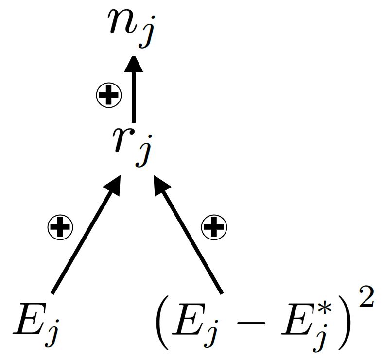
Causal diagrams (Fig. 3, 4, 5, 7, 9) can be used to demonstrate how each coexistence mechanism
operates. With the exception of density-independent effects (∆Ei ), each coexistence mechanism has
two features: 1) a negative feedback loop involving population density, and 2) some degree of spe-
cialization / exclusivity / ecological differentiation. For example, in the causal diagram for the linear
density-dependent effects, ∆ρi (Fig. 4), species j has a species-specific competition parameter Cj , im-
plying that species j specializes on particular resources or natural enemies. In the causal diagram for
the storage effect, ∆Ii , (Fig. 7), specialization manifests as the species-specific environmental parame-
ter, Ej . Note that the causal diagrams are highly stylized; they focus on a feedback loop corresponding
to a single species, and therefore only show a small subset of a much larger community-level causal
diagram.
There are at least two reasons for relating simple explanations for coexistence to the coexistence
mechanisms. First, the resulting taxonomy of models can serve as a heuristic guide for determining
the precise causes of coexistence in a new model. Second, we need to multiple, disparate models
to give a fully generally interpretation of coexistence mechanisms. As we will see, it is likely that
some misconceptions about relative nonlinearity and the storage effect are the consequence of over-
generalizing from two highly-similar models (the lottery model and the annual plant model; Chesson,
1994).
19Figure 3: Density-independent effects. The density-independent factors (captured by Ej and Var (Ej ))
affect growth rates and population density. Note the absence of any feedback loops. The quantity
2
Ej − Ej∗ becomes Varx,t (Ej ) when averaged across space and time; see Eq.3 and Eq.6 in Section 3.
.
4.1 ∆Ei : Density-independent effects
The first coexistence mechanism, ∆Ei , is termed density-independent effects and can be interpreted
as the degree to which density-independent factors favor the invader. The value of ∆Ei does not
depend on any species’ density. This represented by the lack of a feedback loop in clearly in Figure
3. Consequentially, one species will have the largest ∆Ei , regardless of which species is the invader; if
all other terms in the invasion growth rate partition are zero, then all other species in the community
will be excluded (Chesson and Huntly, 1997). This thought experiment demonstrates 1) that density-
dependent factors are necessary for coexistence and therefore ∆Ei might rightfully not deserve the
title of "coexistence mechanism"; and 2) why all the Taylor series terms (of the average growth rate
decomposition, Eq.6) containing only Ej ’s are shunted into ∆Ei , while the growth rate components
containing only Cj ’s are split between ∆ρi and ∆Ni : the density-independent effects are between-
species differences that cannot be responsible for coexistence, so it is often uninteresting to partition
them further (but see Ellner et al., 2019).
4.2 ∆ρi : Linear density-dependent effects
The second quantity, ∆ρi , is called the linear density-dependent effects. The linear density-dependent
effects is best understood as the class of classic explanations for coexistence: resource and natural-
enemy partitioning. More precisely, ∆ρi is the rare-species advantage resulting from specialization on
the mean level of density-dependent factors, which could take the form of mineral nutrients, water,
carbon, prey species, light, space, refugia, pathogens, parasites, parasitoids, predators, herbivores, etc.
The "specialization" need not be complete in the sense that each species only affects and is affected
by a single density-dependent factor. Rather, there is some contingent (i.e., model specific) threshold
of specialization needed in order to attain coexistence (Barabás et al., 2016). In the two-species
Lotka-Volterra model, there is a simple mathematical condition for the "specialization threshold" (i.e.,
intraspecific competition > interspecific competition). In more speciose communities, such simple
equations do not generally exist (Saavedra et al., 2017; Logofet, 1993).
Naturally, coexistence in explicit resource-consumer models can be attributed to ∆ρi (e.g., Ellner
et al., 2019). The same can be said of coexistence in Lotka-Volterra-like models (Volterra, 1937; Hassell
and Comins, 1976; Walters and Korman, 1999; Dallas et al., 2021), where species densities themselves
can be treated as density-dependent factors. Lotka-Volterra dynamics are usually viewed as a useful
but imperfect simile for the dynamics associated with competition or apparent-competition (Abrams
20Figure 4: Linear density-dependent effects. The negative feedback loop involves the species-specific
competition parameter Cj , which includes the effects of resources and natural enemies.
et al., 2008; Mayfield and Stouffer, 2017; O’Dwyer, 2018). However, when resource dynamics are fast,
a specific form of resource-consumer dynamics are well-approximated by Lotka-Volterra dynamics
(MacArthur, 1970; Chesson, 1990a).
The linear density-dependent effects encompasses several notable explanations for coexistence.
First, ∆ρi captures coexistence mechanisms that operate on finer-grained spatial or temporal scales
than that of observation/data-collection (more on this in Section 5.17). For example, the competition–
colonization trade-off can be attributed to fitness-density covariance from a "worm’s-eye view" (Bolker
and Pacala, 1999; Shoemaker and Melbourne, 2016), but can be attributed to the linear density-
dependent effects from a "bird’s-eye view". the competition–colonization trade-off (Skellam, 1951;
Levins and Culver, 1971) can be attributed to ∆ρi . The same is true for related explanations, such as
the fecundity-dispersal trade-off (Yu and Wilson, 2001) and a seed size-number trade-off (Turnbull et
al., 1999; Muller-Landau, 2010). The latter factoid can be verified by looking at the equations in Levins
and Culver’s (1971) classic paper on the competition–colonization trade-off and using the process of
elimination to exclude fluctuation-dependent coexistence mechanisms. There are no patch-level equa-
tions, which excludes spatial fluctuation-dependent coexistence mechanisms; and the per capita growth
rate equation is linear and deterministic, which excludes temporal fluctuation-dependent coexistence
mechanisms.
Second, the Janzen-Connell hypothesis of tropical tree coexistence (Janzen, 1970; Connell, 1971)
also falls under the umbrella of ∆ρi . Unlike ordinary natural-enemy partitioning, the Janzen-Connell
hypothesis posits that coexistence is boosted further by distance-responsive predation: parasites and
diseases tend to kill seeds and seedlings which are near to their parent trees. However, Stump and Ches-
son (2015) used MCT to show that distance-responsive predation generally undermines coexistence,
thus disproving the Janzen-Connell hypothesis in its most platonic form.
Finally, coexistence via intransitive competition (Soliveres and Allan, 2018) is partially captured
by ∆ρj . Intransitive competition means that there is no best competitor in all settings, such that
coexistence occurs via indirect effects that span across a network of interspecific interactions. This
process is well-caricatured by Rock-Paper-Scissors dynamics, where species A beats B, B beats C,
C beats A, and so on (May and Leonard, 1975, Gilpin, 1975). Intransitive competition is normally
studied with Lotka-Volterra models, it can also arise in more complex, multi-trophic models (Schreiber
and Rittenhouse, 2004; Schreiber, Patel, et al., 2018). While it has not been documented empirically or
theoretically (to our knowledge), intransitivity can be mediated through other coexistence mechanisms.
For instance, intransitivity via relative nonlinearity may occur if species A generates a lot of resource
variation, which disproportionately hurts species B via relative nonlinearity, and so on.
Invasion analysis is generally seen as incompatible with coexistence via intransitive competition.
21You can also read