Reviews and syntheses: Ongoing and emerging opportunities to improve environmental science using observations from the Advanced Baseline Imager on ...
←
→
Page content transcription
If your browser does not render page correctly, please read the page content below
Biogeosciences, 18, 4117–4141, 2021
https://doi.org/10.5194/bg-18-4117-2021
© Author(s) 2021. This work is distributed under
the Creative Commons Attribution 4.0 License.

Reviews and syntheses: Ongoing and emerging opportunities to
improve environmental science using observations from the
Advanced Baseline Imager on the Geostationary Operational
Environmental Satellites
Anam M. Khan1 , Paul C. Stoy1,2,3,4 , James T. Douglas4 , Martha Anderson5 , George Diak6 , Jason A. Otkin6,7 ,
Christopher Hain8 , Elizabeth M. Rehbein9 , and Joel McCorkel10
1 Nelson  Institute for Environmental Studies, University of Wisconsin – Madison, Madison, WI, USA
2 Department   of Biological Systems Engineering, University of Wisconsin – Madison, Madison, WI, USA
3 Department of Atmospheric and Oceanic Sciences, University of Wisconsin – Madison, Madison, WI, USA
4 Department of Land Resources and Environmental Sciences, Montana State University, Bozeman, MT, USA
5 Hydrology and Remote Sensing Laboratory, ARS USDA, Beltsville, MD, USA
6 Space Sciences and Engineering Center, University of Wisconsin – Madison, Madison, WI, USA
7 Cooperative Institute for Meteorological Satellite Studies, University of Wisconsin – Madison, Madison, WI, USA
8 Short-term Prediction Research and Transition Center, NASA Marshall Space Flight Center,

Earth Science Branch, Huntsville, AL, USA
9 Department of Electrical and Computer Engineering, Montana State University, Bozeman, MT, USA
10 NASA Goddard Space Flight Center, Greenbelt, MD 20771, USA

Correspondence: Anam M. Khan (amkhan7@wisc.edu)

Received: 4 December 2020 – Discussion started: 8 January 2021
Revised: 9 May 2021 – Accepted: 6 June 2021 – Published: 12 July 2021

Abstract. Environmental science is increasingly reliant on      in ecology and environmental science. We review a num-
remotely sensed observations of the Earth’s surface and at-     ber of existing applications that use data from geostationary
mosphere. Observations from polar-orbiting satellites have      platforms and present upcoming opportunities for observing
long supported investigations on land cover change, ecosys-     key ecosystem properties using high-frequency observations
tem productivity, hydrology, climate, the impacts of distur-    from the Advanced Baseline Imagers (ABI) on the Geosta-
bance, and more and are critical for extrapolating (upscal-     tionary Operational Environmental Satellites (GOES), which
ing) ground-based measurements to larger areas. However,        routinely observe the Western Hemisphere every 5–15 min.
the limited temporal frequency at which polar-orbiting satel-   Many of the existing applications in environmental science
lites observe the Earth limits our understanding of rapidly     from ABI are focused on estimating land surface tempera-
evolving ecosystem processes, especially in areas with fre-     ture, solar radiation, evapotranspiration, and biomass burn-
quent cloud cover. Geostationary satellites have observed the   ing emissions along with detecting rapid drought develop-
Earth’s surface and atmosphere at high temporal frequency       ment and wildfire. Ongoing work in estimating vegetation
for decades, and their imagers now have spectral resolutions    properties and phenology from other geostationary platforms
in the visible and near-infrared regions that are compara-      demonstrates the potential to expand ABI observations to es-
ble to commonly used polar-orbiting sensors like the Mod-       timate vegetation greenness, moisture, and productivity at a
erate Resolution Imaging Spectroradiometer (MODIS), Vis-        high temporal frequency across the Western Hemisphere. Fi-
ible Infrared Imaging Radiometer Suite (VIIRS), or Landsat.     nally, we present emerging opportunities to address the rel-
These advances extend applications of geostationary Earth       atively coarse resolution of ABI observations through multi-
observations from weather monitoring to multiple disciplines    sensor fusion to resolve landscape heterogeneity and to lever-

Published by Copernicus Publications on behalf of the European Geosciences Union.
4118 A. M. Khan et al.: Ongoing and emerging opportunities to improve environmental science
age observations from ABI to study the carbon cycle and
ecosystem function at unprecedented temporal frequency.
1 Introduction
Modern environmental science would be unrecognizable
without satellite remote sensing, which has revolutionized
our field since its advent over a half-century ago (Kerr
and Ostrovsky, 2003). The platforms by which we observe
the Earth system are increasingly diverse and now include
miniaturized satellites (CubeSats), sensors like the ECOsys-
tem Spaceborne Thermal Radiometer Experiment on Space
Station (ECOSTRESS) traveling on board the International
Space Station (Hulley et al., 2017), and even lidar systems
(Coyle et al., 2015; Qi et al., 2019), yet most environmental
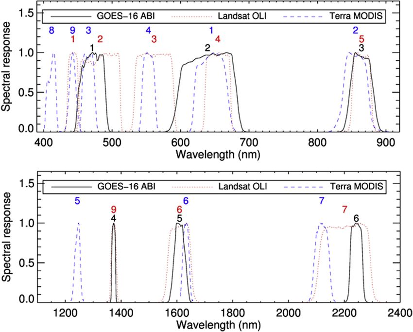
science applications employ polar-orbiting satellites, namely Figure 1. A comparison of the spectral sensitivity of the Advanced
Landsat and the Moderate Resolution Imaging Spectrora- Baseline Imager (ABI) with the Landsat Operational Land Imager
(OLI) and MODIS Terra (McCorkel et al., 2020).
diometer (MODIS). The Landsat and MODIS programs have
radically improved the ability of ecologists to track vegeta-
tion change and its impacts on habitat, biogeochemical cy-
cling, and other ecosystem services (De Araujo Barbosa et sat and MODIS (Table 1; Fig. 1). Given the constellation of
al., 2015). Like all remote sensing platforms, polar-orbiting geostationary satellites around the world, extending environ-
satellites must make compromises with respect to spectral mental science applications to ABI and generating relevant
resolution, spatial scale, and temporal scale that limit their data products is crucial for achieving near-global coverage
ability to measure all things, all the time. Notably, the 1 to 2 d of satellite environmental data available at the timescale of
cadence of MODIS and Visible Infrared Imaging Radiometer minutes. Developing algorithms that can be applied to data
Suite (VIIRS) and 3 to 5 d cadence of the combined Landsat- from multiple geostationary satellites will be an important
and Sentinel-2-class sensors may be insufficient for tracking component for achieving near-global coverage.
ecological phenomena that occur at shorter timescales, in- Here, we detail a number of applications by which GOES
cluding the timing of rapid environmental change (White et and other geostationary satellites have enhanced or could en-
al., 2009) and the diurnal behavior of land surface function, hance our understanding of ecological phenomena that oc-
such as sub-hourly variations in ecosystem carbon and water cur at timescales as short as minutes. We keep our focus on
fluxes (Chudnovsky et al., 2004; Grant et al., 2000). the GOES constellation, but we also discuss research and ap-
As a part of the European Organisation for the Exploita- plications from various satellites in the global constellation
tion of Meteorological Satellites (EUMETSAT), the Satellite of geostationary satellites to provide the larger context for
Application Facility for Land Surface Analysis (LSA SAF) emerging applications from GOES ABI. We outline the tech-
has leveraged high frequency observations from the Spinning nical steps necessary to make imagery from ABI more useful
Enhanced Visible and Infrared Imager (SEVIRI) on board the for environmental science, with an eye toward near real-time
Meteosat Second Generation (MSG) geostationary satellites monitoring of environmental phenomena across the globe.
to provide operational products relevant for studying vegeta- We also note complementarity between GOES and other
tion, wildfires, the surface radiation budget, and the carbon geostationary platforms, including Japan’s Himawari-8/9,
and water cycle (Trigo et al., 2011) at sub-daily timescales. South Korea’s GEO-KOMPSAT-2A, and European Union
These opportunities are also available in the Western Hemi- Meteosat satellites – especially the forthcoming third gener-
sphere. Focusing on the Advanced Baseline Imager (ABI), ation (Meteosat Third Generation, MTG) – all of which have
a joint effort by the National Oceanic and Atmospheric similar spectral resolution that make near-global observation
Administration (NOAA) and the National Aeronautics and possible (Table 1). We first review the recent efforts regard-
Space Association (NASA) on board the Geostationary Op- ing geolocation and atmospheric correction to produce sur-
erational Environmental Satellites (GOES), we argue that the face reflectance from ABI and other geostationary imagers.
GOES constellation – commonly used as weather satellites – We then describe new data products that can be created us-
represents an underexplored opportunity for environmental ing state-of-the-art geostationary satellite data, with a brief
science in situations where spatial resolution can be com- description of existing data products that are providing key
promised in favor of more frequent imagery, especially now insight into Earth surface processes. Finally, we outline ex-
that ABI’s spectral sensitivity has approached that of Land- isting and emerging applications of observations from geo-
Biogeosciences, 18, 4117–4141, 2021 https://doi.org/10.5194/bg-18-4117-2021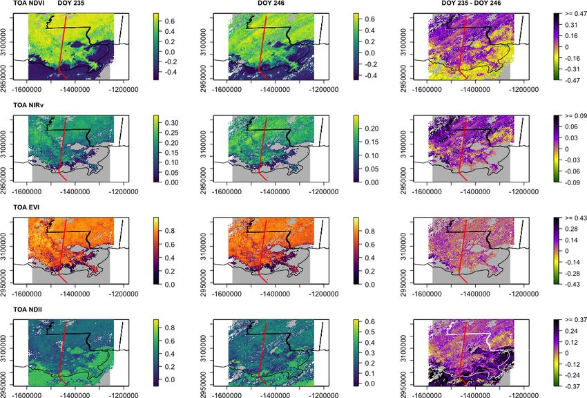
A. M. Khan et al.: Ongoing and emerging opportunities to improve environmental science                                    4119

stationary satellites that are ushering in the era of “hyper-   lects a CONUS scene every 5 min and two mesoscale scenes
temporal” remote sensing (Miura et al., 2019) for environ-      every minute in the flex mode (Schmit and Gunshor, 2020).
mental science.                                                    In late April 2018, an issue with the GOES 17 ABI cool-
                                                                ing system was detected due to malfunctioning of the loop
                                                                heat pipe which transfers heat from the ABI detectors and
2     Background                                                helps maintain adequate temperatures for proper function-
                                                                ing (Yu et al., 2019). This resulted in the loss of infrared
2.1    Geostationary satellites: past, present, and future      data during some nighttime hours, around 13:30 UTC, dur-
                                                                ing parts of the year due to the Sun heating the seven ABI
Geostationary remote sensing began with the launch of           detectors faster than they can be cooled, resulting in infrared
six Applications Technology Satellites (ATS), starting in       emissions from the overheated detectors (NOAA and NASA,
1966 (Suomi and Parent, 1968). The subsequent success-          2020; NOAA, 2020). This nighttime data loss can also fluc-
ful launches of the Synchronous Meteorological Satellites       tuate seasonally, depending on how much solar radiation the
(SMSs) were the precursor to the GOES mission, which be-        instrument absorbs (NOAA, 2020). A data quality flag in
gan in 1974 and continues to the present (Menzel, 2020).        the metadata of the Level 1b Radiances and Level 2 Cloud
By 1979, the global constellation of geostationary satel-       and Moisture Imagery can identify the faulty nighttime data
lites included the European Space Agency’s Meteosat, the        (NOAA and NASA, 2020). This malfunction will result in
Japanese Geostationary Meteorological Satellite (GMS), and      the loss of some nighttime data for data products that utilize
two GOES (Menzel, 2020). In total, 17 GOES have been suc-       the infrared bands and are relevant for observing the full di-
cessfully sent to space as of 2018, two of which – GOES-16,     urnal cycle.
positioned at 75.2 W (currently GOES-East), and GOES-17,
positioned at 137.2 W (currently GOES-West) – arise from
the GOES-R series that include additional visible and near-     3     ABI top-of-atmosphere data to surface reflectance
IR channels that are commensurate with channels observed              and surface temperature
by Landsat and MODIS (Table 1; Fig. 1). The GOES-R series
has an expected operational lifetime to 2036, which promises    The ABI collects top-of-atmosphere (TOA) data from a given
multiple years of continuous data availability. This will be    location at a constant view zenith angle (VZA) and vary-
followed by the Geostationary and Extended Orbits program,      ing solar zenith angles (SZA) throughout the day. While
which is planned for operation in 2030–2050 and is antic-       the increased sampling of SZA creates opportunities in sur-
ipated to include “GOES-R-class” imagers (Sullivan et al.,      face bidirectional reflectance factor (BRF) modeling (Ma et
2020).                                                          al., 2020), the large VZA at off-nadir locations can present
                                                                challenges for studying the land surface, including coars-
2.2    Advanced Baseline Imager (ABI)                           ened resolution, potentially degraded locational accuracy,
                                                                and more complex atmospheric compensation due to longer
The ABI is the primary instrument on board GOES-16/17           slant paths. Below, we review the existing efforts to address
and is designed for monitoring land and ocean surfaces, the     these challenges and make ABI imagery more suitable for
atmosphere, and cloud formation (Schmit et al., 2017, 2018).    studying the land surface.
The ABI has 16 spectral bands that measure solar reflected
radiance in the visible and near-infrared wavelengths and       3.1    Geolocation
emitted radiance at infrared wavelengths (Schmit and Gun-
shor, 2020). With multiple infrared bands positioned in at-     The geolocation accuracy of ABI on GOES-16 and GOES-
mospheric absorption regions and in atmospheric windows,        17 has been tracked and improved throughout its provisional
the ABI can collect information from the Earth’s surface        and operational stages using the Image Navigation and Reg-
and multiple levels in the atmosphere (Schmit and Gun-          istration (INR) Performance Assessment Tool Set (IPATS;
shor, 2020). Multiple scan modes are used to provide near-      Tan et al., 2018, 2019, 2020). IPATS quantifies the naviga-
hemispheric geographic coverage, with spatial resolutions       tion error, i.e., the difference between the location of a pixel
between 0.5 and 2 km. The full disk scene consists of near-     in ABI imagery and a reference location (Tan et al., 2020).
hemispheric coverage centered at the Equator and the lon-       Some of the largest navigation errors, calculated from cor-
gitude of the sensing satellite (DOC, NOAA, NESDIS, and         relations between subsets of ABI and Landsat 8 imagery
NASA, 2019). The ABI also scans a scene of the con-             concentrated along the coast of North and South America,
tiguous United States (CONUS) and two mesoscale scenes          were 10–13 µrad less than the mission requirement of 28 µrad
(1000 km×1000 km). Operating in the flex mode, the ABI          (1 km at nadir) in October 2019 (Tan et al., 2020). In ad-
collected a full disk image every 15 min until April 2019 but   dition to IPATS, the Geostationary-NASA Earth Exchange
now collects a full disk image every 10 min (with the excep-    (GeoNEX) processing chain adjusts the geolocation of ABI
tion of GOES-17 during parts of the year). The ABI also col-    imagery using a reference map from the Shuttle Radar Topo-

https://doi.org/10.5194/bg-18-4117-2021                                                Biogeosciences, 18, 4117–4141, 2021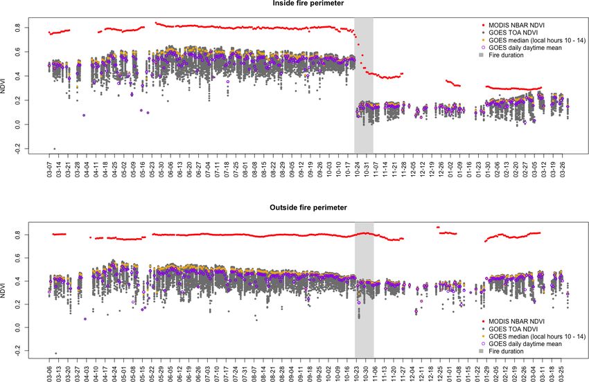
4120                          A. M. Khan et al.: Ongoing and emerging opportunities to improve environmental science

Table 1. Instrument characteristics for the GOES-R Advanced Baseline Imager, Advanced Himawari Imager on Himawari-8/9, and the
Advanced Meteorological Imager on the Geostationary – Korea Multi-Purpose Satellite-2 (GEO-KOMPSAT-2A) (a) and the Global Ocean
Color Imager-II (GOCI-II) on GEO-KOMPSAT-2B (b).

              (a)
                       GOES-16/17                            Himawari-8/9                 GEO-KOMPSAT 2A
                     Advanced Baseline                     Advanced Himawari             Advanced Meteorological
                       Imager (ABI)                          Imager (AHI)                    Imager (AMI)
              Band       Central       Spatial   Band           Central      Spatial   Band      Central      Spatial
                      wavelength    resolution               wavelength   resolution          wavelength   resolution
                            (µm)         (km)                      (µm)        (km)                 (µm)        (km)
              1              0.47           1          1           0.47            1      1         0.47             1
                                                       2           0.51            1      2         0.51             1
              2              0.64         0.5          3           0.64          0.5      3         0.64           0.5
              3              0.86           1          4           0.86            1      4         0.86             1
              4              1.37           2                                             5          1.4             2
              5               1.6           1          5            1.6           2       6          1.6             2
              6               2.2           2          6            2.3           2
              7               3.9           2          7            3.9           2       7          3.8            2
              8               6.2           2          8            6.2           2       8          6.2            2
              9               6.9           2          9            6.9           2       9          6.9            2
              10              7.3           2         10            7.3           2      10          7.3            2
              11              8.4           2         11            8.6           2      11          8.6            2
              12              9.6           2         12            9.6           2      12          9.6            2
              13             10.3           2         13           10.4           2      13         10.4            2
              14             11.2           2         14           11.2           2      14         11.2            2
              15             12.3           2         15           12.4           2      15         12.4            2
              16             13.3           2         16           13.3           2      16         13.3            2

                                                 (b)
                                                           GEO-KOMPSAT 2B
                                                           Global Ocean Color
                                                           Imager-II (GOCI-II)
                                                 Band           Central      Spatial
                                                             wavelength   resolution
                                                                   (nm)         (m)
                                                 1                 380           250
                                                 2                 412           250
                                                 3                 443           250
                                                 4                 490           250
                                                 5                 510           250
                                                 6                 555           250
                                                 7                 620           250
                                                 8                 660           250
                                                 9                 680           250
                                                 10                709           250
                                                 11                745           250
                                                 12                865           250
                                                 13           Wideband           250

Biogeosciences, 18, 4117–4141, 2021                                                      https://doi.org/10.5194/bg-18-4117-2021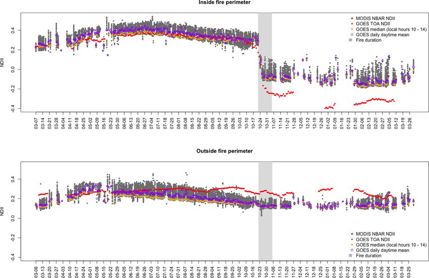
A. M. Khan et al.: Ongoing and emerging opportunities to improve environmental science                                       4121

graphic Mission (SRTM) digital elevation model (DEM) and            tion of MODIS imagery, the Multi-Angle Implementation of
more than 30 000 landmarks along coastlines (Wang et al.,           Atmospheric Correction (MAIAC) has also been adapted to
2020). The shift in the geolocation of the red band (500 m at       provide provisional daytime surface reflectance every 10 min
nadir) between IPATS and the GeoNEX algorithm was under             for bands 1–6 of the AHI with plans to extend the algorithm
0.5 pixels for a majority of the time throughout the full disk      to ABI (Li et al., 2019b). The surface reflectance from the
scene but can be as large as 1–2 pixels for short periods of        AHI showed less variation compared to surface reflectance
time (Wang et al., 2020).                                           from MODIS and the differences in surface reflectance be-
                                                                    tween the AHI and MODIS were smaller for the red, near-
3.2     Parallax                                                    infrared (NIR), and shortwave infrared (SWIR) bands com-
                                                                    pared to the blue and green bands (Li et al., 2019b). ABI
Geostationary satellites observe most of the hemisphere at an       channels 1, 3, 5, and 6 are accurate to within 2 %, but channel
angle relative to the zenith, which introduces a challenge due      2 has a bias error of up to 5 % (McCorkel et al., 2020). With
to parallax, i.e., the effect of observing an object from a large   geolocation, parallax, atmospheric correction, and sensor ac-
VZA. Parallax can result in uncertainties in land surface ob-       curacy taken into account, imagery from the ABI can provide
servations in mountainous terrain and can introduce errors          sub-hourly estimates of various land surface variables.
in the mapped location of clouds (Bieliński, 2020). These er-
rors vary by VZA and the height of the feature and are largest      3.3.2   Surface temperature
for high VZA and high feature altitude relative to the surface
(Bieliński, 2020; Zakšek et al., 2013). For example, the par-      Atmospheric attenuation due to water vapor requires atmo-
allax shift at 49◦ latitude from GOES-16 ABI can be as large        spheric correction of thermal data collected from satellites
as 51 km for an object that is 15 km high (Whittaker, 2014).        and also limits surface temperature retrieval to thermal bands
Since the mapped location of the clouds detected depends, in        that have the lowest atmospheric absorption (Sun and Pinker,
part, on the VZA, parallax shifts can also complicate com-          2003). A single-channel approach requires the use of one
paring the location of clouds between sensors with different        thermal channel within an atmospheric window at around
VZA (Zakšek et al., 2013). However, it is possible to correct       10 µm and radiative transfer modeling to simulate atmo-
for parallax shifts with knowledge of VZA and feature (cloud        spheric transmittance and emission of longwave radiation
or surface) altitude (Kim et al., 2017; Yeom et al., 2020).         (Li et al., 2013; Pinker et al., 2019). With known land sur-
                                                                    face emissivity and atmospheric profiles and simulated atmo-
3.3     Atmospheric correction                                      spheric transmittance/emission, surface temperature can be
                                                                    retrieved through the inversion of a radiative transfer equa-
3.3.1    Surface reflectance                                        tion that explains the different components of at-sensor ra-
                                                                    diance (Li et al., 2013). Since accurate atmospheric profiles
Correcting for atmospheric attenuation of radiation to derive       over a study area can be difficult to obtain, a split-window
surface reflectance from TOA reflectance is a crucial prereq-       technique can be used to correct atmospheric absorption to
uisite for studying surface processes from satellite platforms.     estimate surface temperature from at-sensor radiance in two
Current efforts to estimate surface reflectance from the ABI,       thermal bands with differential water vapor absorption (Li
the Advanced Himawari Imager (AHI), and the Geostation-             et al., 2013; Ulivieri and Cannizzaro, 1985). Split-window
ary Ocean Color Imager (GOCI) on board the Communica-               techniques were used in earlier estimates of surface temper-
tion, Ocean, and Meteorological Satellite (COMS) include            ature from GOES thermal data, and they are based on the
generating lookup tables from the Second Simulation of the          relationship between surface temperature and the difference
Satellite Signal in the Solar Spectrum (6S) radiative transfer      in temperature between two adjacent thermal bands with high
model (He et al., 2019; Tian et al., 2010; Vermote et al., 1997;    emissivity and low atmospheric absorption typically centered
Yeom and Kim, 2015; Yeom et al., 2018, 2020). Optimal es-           at 11 and 12 µm (Li et al., 2013; Sun and Pinker, 2003).
timation methods that estimate surface BRF from SEVIRI              The split-window techniques used to generate the GOES-R
have been extended to estimate surface broadband albedo and         hourly land surface temperature (LST) product is discussed
surface reflectance from the ABI and the AHI on Himawari-           in Sect. 4.4, which further expands on surface temperature
8 (Govaerts et al., 2010; He et al., 2019, 2012; Wagner et          retrieval from GOES. In Sect. 4.4, we also discuss the impor-
al., 2010). These algorithms estimate surface reflectance and       tance of emissivity for estimating LST and current sources of
broadband surface albedo by minimizing the difference be-           emissivity estimates used in LST retrievals from geostation-
tween TOA BRF estimated through radiative transfer mod-             ary satellites.
eling and measured by the satellite (He et al., 2019, 2012).           Similar to surface reflectances, the directional thermal ra-
Unlike the surface reflectance algorithm currently used for         diation recorded by sensors on satellites can also be im-
SEVIRI, the algorithm for the ABI and the AHI takes the             pacted by the VZA of the sensor (Diak and Whipple, 1995).
diurnal variation in aerosol optical depth into account (He         Products that utilize diurnal thermal data from GOES have
et al., 2019). Originally developed for atmospheric correc-         used the difference in surface radiometric temperature dur-

https://doi.org/10.5194/bg-18-4117-2021                                                    Biogeosciences, 18, 4117–4141, 2021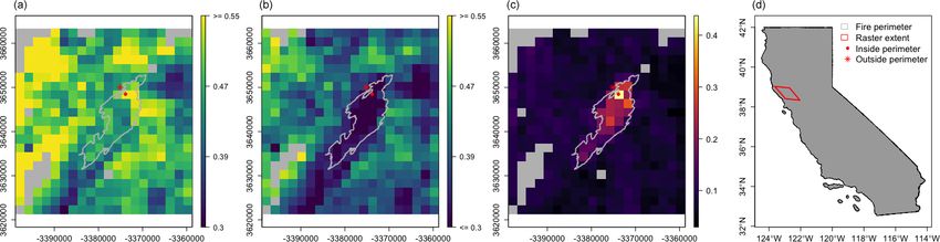
4122                           A. M. Khan et al.: Ongoing and emerging opportunities to improve environmental science

ing the morning hours, which has shown to be less sensitive           Incident solar radiation in the wavelengths of photosyn-
to changes in VZA compared to absolute surface radiomet-           thetically active radiation (PAR; 400–700 nm) can also be
ric temperature (Anderson et al., 1997; Diak and Whipple,          estimated using the visible bands of geostationary satellites
1995). Other methods that address the impacts of varying           (Janjai and Wattan, 2011). Specifying a range of SZA, VZA,
VZA include adding zenith angle correction terms to split-         cloud types, aerosol types, cloud extinction coefficient, and
window algorithms in order to address the large path lengths       atmospheric visibility, lookup tables generated from simu-
at high VZA (Sun and Pinker, 2003; Yu et al., 2009).               lations of Moderate Resolution Atmospheric Transmission
                                                                   (MODTRAN) have been used to estimate downwelling PAR
                                                                   from at-sensor radiance (Zhang et al., 2014; Zheng et al.,
4     Data products                                                2008). These methods have been extended to multiple geo-
                                                                   stationary satellites, including GOES-11 and GOES-12 and
Geostationary satellites can now measure a number of com-
                                                                   MODIS surface reflectance data, to generate global incident
mon vegetation indices used for ecological applications and
                                                                   PAR estimates (Zhang et al., 2014).
make measurements that support derived products, including
                                                                      Although these methods account for elevation, validation
land surface temperature, as noted, incident solar radiation,
                                                                   efforts have shown that satellite-derived PAR in high-altitude
and more. We describe these measurements with an eye to-
                                                                   areas can be biased when compared to ground measure-
ward explaining the benefits and challenges of using geosta-
                                                                   ments, possibly due to the inaccurate specification of atmo-
tionary platforms such as the ABI for ecology and environ-
                                                                   spheric profiles governing water vapor corrections (Zhang et
mental science.
                                                                   al., 2014). Furthermore, PAR estimated from satellites has
4.1    Incident solar radiation and photosynthetically             been reported to underestimate PAR measured on the ground
       active radiation (PAR)                                      when the model assumed urban aerosol absorption over ar-
                                                                   eas where maritime aerosols were more dominant (Janjai and
Geostationary satellites are equipped to estimate incident so-     Wattan, 2011). Despite these limitations, frequent estimates
lar radiation at the Earth’s surface (Diak, 2017; Pinker et al.,   of PAR and incident solar radiation from geostationary satel-
2002), critical for the surface energy balance, photosynthe-       lites may be uniquely suited to drive the land surface mod-
sis, and solar power applications. Earlier efforts to do so in-    els that are operating at increasingly fine spatial and tempo-
clude a simple physical model by Gautier et al. (1980), which      ral resolutions, providing a natural link for using geostation-
estimated incident solar radiation during clear and cloudy         ary satellite observations to improve our understanding of the
conditions using the reflectance from the visible band of the      carbon, water, and energy cycles (Williams et al., 2009).
Visible Infrared Spin-Scan Radiometer (VISSR) on GOES-                Terrestrial photosynthesis is particularly responsive to dif-
2. The model included Rayleigh scattering and water vapor          fuse PAR, which penetrates plant canopies more efficiently
absorption of downwelling and reflected shortwave radiation.       than direct PAR (Emmel et al., 2020; Gu et al., 2003). The
Cloud albedo and absorption were estimated from a linear re-       diffuse fraction of incoming PAR is well-described as a lin-
lationship with the satellite-measured cloud reflectance, and      ear function of transmissivity, or a clearness index, through
estimates of incident solar radiation were subsequently im-        the atmosphere within certain inflection points (Erbs et al.,
proved by including ozone absorption of shortwave radia-           1982; Oliphant and Stoy, 2018; Weiss and Norman, 1985).
tion in the atmosphere (Diak and Gautier, 1983; Diak, 2017).       Estimates of cloud height, optical depth, and particle size,
Continued improvements in both the physical model and              along with aerosols from GOES, can be used to further parti-
the spatiotemporal resolution of the GOES imagery have re-         tion incoming PAR into direct and diffuse beam fractions as
sulted in higher accuracy of hourly and daily insolation esti-     currently provided by EUMETSAT at 15 min intervals (Car-
mates when compared to pyranometer measurements (Diak,             rer et al., 2019). Such observations could ultimately prove
2017; Otkin et al., 2005). More recent models of the trans-        useful for analyses of the diurnal pattern of carbon cycling
mittance of direct and diffuse shortwave radiation through         (see Sect. 6.1), given that the variability in terrestrial carbon
aerosol extinction by different aerosol components, gaseous        cycling is often most sensitive to the variability in PAR at
absorption, and Rayleigh scattering have provided estimates        timescales from minutes to days (Stoy et al., 2005).
of the surface shortwave radiation flux and its diffuse fraction
from SEVIRI observations at 15 min resolution (Carrer et al.,      4.2   Vegetation greenness
2019) and could also be applied to ABI observations. Apply-
ing algorithms for estimating incident solar radiation to data     The normalized difference vegetation index (NDVI) – the
from multiple geostationary satellites can lead to near-global     normalized difference between the reflectance in red and
coverage and be beneficial for near-global estimates of evap-      near-infrared wavelengths – is strongly correlated to chloro-
otranspiration and gross primary productivity that are driven,     phyll content, green biomass, leaf area index (LAI), and the
in part, by solar radiation.                                       fraction of incoming PAR absorbed by leaves (fAPAR; Ga-
                                                                   mon et al., 1995; Jordan, 1969; Rouse et al., 1974; Running
                                                                   et al., 1986; Tucker, 1979; Tucker et al., 1985) and, there-

Biogeosciences, 18, 4117–4141, 2021                                                   https://doi.org/10.5194/bg-18-4117-2021
A. M. Khan et al.: Ongoing and emerging opportunities to improve environmental science 4123
fore, is a critical variable for monitoring the land surface. wavelengths (1.3–2.5 µm). Reflectance by plants in the
The ABI also has the ability to measure the Enhanced Vege- SWIR has a negative relationship with leaf water content
tation Index (EVI) which is beneficial in areas (and periods) (Chen et al., 2005; Gao, 1996; Tucker, 1980), and multi-
of dense vegetation cover where, unlike NDVI, EVI does not ple vegetation indices have been developed from bands in
saturate and in open canopy areas because of a correction the SWIR wavelengths to capture these phenomena, espe-
factor applied for canopy background (Huete et al., 2002; cially in the 1.55–1.75 µm range (Fensholt and Sandholt,
Zhou et al., 2014). The near-infrared reflectance of vegeta- 2003; Tucker, 1980). Some notable vegetation indices that
tion (NIRv) is strongly correlated to the amount of incom- use SWIR wavelengths are the normalized difference in-
ing PAR absorbed by, plants and therefore, photosynthesis frared index (NDII) and the normalized difference water in-
at half-hourly to annual timescales and has shown stronger dex (NDWI) which have been formulated from the differ-
relationships with photosynthesis compared to NDVI (Badg- ence in reflectance (ρ) in the NIR (0.76–0.9) and SWIR
ley et al., 2017, 2019; Baldocchi et al., 2020; Wu et al., 2020) (1.55–2.5 µm) bands as (ρNIR–ρSWIR) / (ρNIR + ρSWIR)
and can also, in principle, be measured by GOES (Table 1). (Chen et al., 2005; Fensholt and Sandholt, 2003; Gao, 1996;
LAI from SEVIRI is produced on a daily and 10 d basis Hardisky et al., 1983; Tucker, 1980). NDII has been used to
through the LSA SAF program (Trigo et al., 2011). High improve global estimates of canopy water content and has
temporal estimates of LAI from ABI will have widespread provided more realistic estimates of canopy water content
utility in the Western Hemisphere by providing an important in semiarid shrublands when compared to regression mod-
variable needed for modeling seasonal vegetation dynamics els without NDII (García-Haro et al., 2020). NDWI has been
and energy, water, and carbon fluxes (Anderson et al., 2011; useful in estimating the water content of corn (maize) fields
Guan et al., 2014; Robinson et al., 2018). An ABI LAI prod- because it saturates at higher values than NDVI in response
uct can provide harmony in temporal scales and data sources to changing vegetation water content during the growing sea-
needed to estimate the fractional vegetation cover needed for son (Chen et al., 2005; Jackson et al., 2004). The short-
a two-source energy balance model used for estimating evap- wave infrared water stress indices derived from MODIS have
otranspiration from GOES thermal data (further discussion stronger correlations with growing season soil moisture than
in Sect. 5.1; Anderson et al., 2011). Similarly, the ABI LAI NDVI in the semiarid grasses of northern Senegal, Africa
product can provide a data source for plant respiration mod- (Fensholt and Sandholt, 2003). Many of these indices and
eling (see further discussion in Sect. 6.1; Robinson et al., their changes over time can now, in principle, be measured
2018). by geostationary satellites (Table 1).
The increased temporal frequency of measurements avail- The ABI, along with the Advanced Meteorological Im-
able from geostationary satellites compared to polar-orbiting ager (AMI) on GEO-KOMPSAT-2A, the AHI, and SEVIRI
satellites provides more opportunities for measuring NDVI, all offer bands in the SWIR regions, with ABI band 5
EVI, LAI, and NIRv in areas with frequent cloud cover placed in the refined interval of 1.55–1.75 µm identified by
(Miura et al., 2019). However, the geostationary position Tucker (1980; Table 1). Atmospherically corrected surface
captures reflected radiation at varying SZA throughout the reflectances from ABI, SEVIRI, AHI, and AMI can provide
day, and these novel Sun–sensor geometries, not previously near-real-time and near-global coverage for vegetation wa-
captured by polar orbiting satellites, can cause diurnal vari- ter content. This remains a relatively unexplored opportunity
ation in vegetation indices calculated from TOA reflectance given the potential benefits of near-real-time monitoring of
(Tran et al., 2020). EVI shows less SZA-induced diurnal vari- vegetation status (Verger et al., 2014).
ation compared to NDVI and is less impacted by the midday
hot spot effect during times of the year (spring and autumn 4.4 Land surface temperature
equinox) when the SZA and AHI VZA are aligned (Tran
et al., 2020). NDVI measurements can be normalized to a The ABI features three longwave infrared bands with spatial
reference Sun–target–sensor geometry by estimating bidirec- resolutions of about 2 km for measuring land surface temper-
tional reflectance distribution functions (BRDFs) to address ature (LST) – the skin temperature of the uppermost layer
the impacts of varying Sun–sensor geometry (Fensholt et al., of the land surface – including correction for atmospheric
2006; Seong et al., 2020; Tian et al., 2010; Yeom and Kim, moisture (Yu et al., 2012). Since the emission from the land
2015; Yeom et al., 2018). Given the SZA sensitivity of NDVI surface diverges from a blackbody, the knowledge of land
measurements, Wheeler and Dietze (2019) demonstrated a surface emissivity is a crucial component for the retrieval of
Bayesian model to estimate a daily midday NDVI value from LST from at-sensor radiance (Li et al., 2013; Sun and Pinker,
diurnal NDVI calculations using ABI observations. 2003). Global emissivity data may be gathered by consult-
ing compiled tables of emissivities for various land covers
4.3 Vegetation moisture along with land cover classifications of the landscape (Li
et al., 2013). Land surface emissivity can also be estimated
Liquid water absorption influences reflectance by plants in through its relationship with the NDVI. This method only
the atmospheric windows of shortwave infrared (SWIR) applies to vegetation and soil and requires knowledge about
https://doi.org/10.5194/bg-18-4117-2021 Biogeosciences, 18, 4117–4141, 20214124 A. M. Khan et al.: Ongoing and emerging opportunities to improve environmental science
the fractional cover of vegetation in a pixel (Li et al., 2013). of Norman et al. (1995). ALEXI models the growth and sen-
Furthermore, land surface emissivities can be estimated by sible heating of the atmospheric boundary layer based on the
using surface temperature–emissivity separation techniques morning rise in surface radiometric temperature that can be
applied to multispectral thermal satellite observations (Li et measured by GOES, estimating time-integrated latent heat
al., 2013). Data sources for land surface emissivity in LST re- flux (or ET, in units of mass flux) as a residual to the over-
trievals from geostationary satellites can include spectral li- all energy balance (Anderson et al., 1997). The model per-
braries given a specific type of environmental surface (Peres forms best when the insolation inputs are also derived from
and DaCamara, 2005), the MODIS operational land surface geostationary satellite data (Sect. 4.1), giving optimal spa-
emissivity product (MOD11), or the Combined ASTER and tial and temporal correspondence between net radiation forc-
MODIS Emissivity over Land (CAMEL) product (Pinker et ings and surface temperature response signals. In comparison
al., 2019). with other sources of insolation data, geostationary-based in-
The hourly ABI LST product uses the difference between solation could significantly improve ET retrievals, particu-
the brightness temperatures of ABI bands 14 (11.2 µm) and larly in areas of frequent cloud cover where reanalysis esti-
15 (12.3 µm) in a split-window algorithm with an added term mates may not accurately capture the timing and spatial ex-
to correct for path length at high view zenith angles (Yu et tents of clouds (Anderson et al., 2019; Wonsook et al., 2020).
al., 2009, 2012). These bands were chosen because they are ALEXI-based ET estimates are produced routinely at 4 km
placed in regions of maximum surface emission with low at- resolution for the United States (Anderson et al., 2020). Also,
mospheric absorption (Yu et al., 2009). However, water vapor daily 2 km resolution ALEXI-based ET estimates have been
absorption in a more moist atmosphere (e.g., a water vapor generated from ABI observations as part of the GOES ET
content greater than 2 g cm−2 ) at large view zenith angles and Drought (GET-D) product system (Fang et al., 2019). A
(>45◦ ) remains an issue for the ABI LST algorithm (Yu et surface energy balance approach has also been used to esti-
al., 2009). mate 30 min ET from albedo and downwelling radiation from
For the generation of a consistent, long-term record of MSG SEVIRI over the areas covered by MSG and 3 h ET in
LST, a single channel approach has also been proposed for the Haihe River Basin in China from hourly LST observa-
LST retrieval from GOES 12 channel 4 (10.7 µm) in order tions from MTSAT (Multifunctional Transport Satellites), a
to develop an algorithm that can be applied to data from Japanese geostationary satellite (Ghilain et al., 2011; Zhao et
multiple GOES satellites, including for time periods from al., 2019). By measuring LST, geostationary satellites can es-
mid-2004–2017 when only one thermal channel was avail- timate sensible heat flux and, therefore, also the Bowen ratio,
able (Pinker et al., 2019). Diurnal LST time series available which can give insight into atmospheric boundary layer heat
from geostationary platforms have a wide range of applica- and moisture transport, as well as plant water stress (Diak
tions in environmental monitoring, from mapping surface– and Whipple, 1995). Applications of ALEXI-based ET and
atmosphere fluxes of heat, water, and carbon dioxide to track- energy fluxes for drought monitoring and modeling carbon
ing drought and fire dynamics. These and other applications fluxes are discussed below.
are discussed further in the following sections.
5.2 Drought monitoring
5 Existing applications of geostationary satellites for Drought indicators based on remotely sensed thermal obser-
environmental science vations can improve the effectiveness of drought early warn-
ing systems due to their high spatial resolution and the ten-
5.1 Evapotranspiration, latent heat flux, and sensible dency for large decreases in ET to precede visible reductions
heat flux in vegetation biomass during early stages of drought develop-
ment (Anderson et al., 2013a; Otkin et al., 2015). The Evapo-
Diurnal observations from GOES provide multiple estimates rative Stress Index (ESI; Anderson et al., 2013a) is a drought
of directional surface radiometric temperature and down- indicator based on standardized anomalies in the actual-to-
welling solar radiation each day to estimate water and en- reference ET ratio, where actual ET is retrieved with ALEXI
ergy fluxes from the soil and canopy (Diak and Stewart, using the morning LST rise signal, typically obtained from
1989). One approach for estimating evapotranspiration (ET) GOES. ESI has demonstrated the ability to provide early sig-
that is well suited for geostationary implementation is the nals of developing vegetation stress (Anderson et al., 2007b,
Atmosphere–Land Exchange Inverse (ALEXI) model (An- 2013a, 2016; Otkin et al., 2015, 2018a).
derson et al., 1997, 2007a; Mecikalski et al., 1999), which A recent prominent application of the ESI has been in the
estimates the bulk surface energy balance (net radiation, sen- detection of flash droughts (Otkin et al., 2013). Flash drought
sible heat flux, latent heat flux, and soil heat flux) and the conditions are characterized by a period of rapid drought in-
nominal partitioning of these fluxes between the soil and tensification and typically include warm air temperature and
canopy. ALEXI is a time-integrated model based on the two- low cloud cover anomalies, with dew point suppressions and
source (vegetation and soil) energy balance (TSEB) approach high winds that can increase ET and hasten the removal of
Biogeosciences, 18, 4117–4141, 2021 https://doi.org/10.5194/bg-18-4117-2021A. M. Khan et al.: Ongoing and emerging opportunities to improve environmental science 4125
water from ecosystems (Gerken et al., 2018; Otkin et al., sions at hourly, daily, and monthly scales (Li et al., 2019a;
2014, 2016, 2018b). ESI has proven to be an effective in- Zhang et al., 2012).
dicator of moisture stress in vegetation and the onset of flash While GOES-R thermal observations can provide biomass
drought conditions (Otkin et al., 2014, 2016, 2018b). For ex- burning emissions at a fine temporal scale, the coarse spa-
ample, rapid temporal changes in the ESI toward increas- tial resolution of GOES-R presents a challenge in detect-
ing vegetation stress appeared several weeks earlier than the ing small sub-pixel fires and emissions. Differences between
point at which the U.S. Drought Monitor (USDM) classified medium (20 m) and coarse resolution (500 m) imagery can
regions of the central United States to be experiencing mod- result in substantial differences in total detected burned area,
erate to exceptional drought in 2003 and 2012 (Otkin et al., estimated emissions, and the length of the fire season (Ramo
2014). The ESI was also able to capture the onset of vege- et al., 2021). Small fires can make up a great portion of total
tation stress and the subsequent vegetation recovery during burned area and emissions, and they can result in a lengthen-
the flash drought and flash recovery sequence of 2015 in the ing of the fire season in regions where anthropogenic fires are
south central United States (Otkin et al., 2019). prevalent (Ramo et al., 2021). Similar to other coarse-spatial-
Drought indices based on precipitation and atmospheric scale emissions datasets, emissions from GOES-R should be
demand highlight areas with the potential for vegetation considered conservative in areas with substantial undetected
stress, but these stresses may not materialize due, for ex- small fires (Ramo et al., 2021). Similar to Ramo et al. (2021),
ample, to beneficial rainfall, management (e.g., irrigation), studies comparing biomass burning emissions from GOES-
or plant root access to groundwater. ESI uses LST to diag- R with emissions from finer spatial resolution satellite im-
nose actual stress materializing on the ground and, there- agery should reveal the magnitude of differences and trade-
fore, has been used as a moisture stress indicator for es- offs between high temporal and spatial resolution in estimat-
timating drought impacts on crop yields (Anderson et al., ing emissions.
2016; Mladenova et al., 2017). ESI is routinely generated
at 4 km resolution over the CONUS, and 5 km globally, or 5.4 Plant phenology
can be downscaled to sub-field or stand scales (30 m) us-
ing higher resolution thermal data from Landsat (Yang et al., Plant canopies have unique and observable events that oc-
2018, 2020). The ability of ESI to detect drought stress ear- cur annually as a part of their phenology. The phenology of
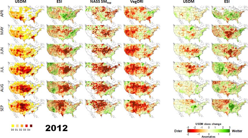
lier than USDM and other indices is shown in Fig. 2 (adapted photosynthesis and plant growth is sensitive to temperature,
from Anderson et al., 2013b). precipitation, and photoperiod (Bauerle et al., 2012; Fu et al.,
2017; Piao et al., 2019; P. C. Stoy et al., 2014), and shifts in
the phenology of carbon uptake and plant growing season
5.3 Wildfire detection and biomass burning emissions
in response to changing climate have important implications
for ecosystems (Bradley et al., 1999; Xu et al., 2020). These
The Automated Biomass Burning Algorithm (ABBA) was shifts often occur on timescales that cause uncertainty from
developed from the 4 and 11 µm bands of the GOES visible polar-orbiting satellites, especially when cloudy conditions
infrared spin-scan radiometer atmospheric sounder (VAS) to are present during spring in the temperate zone (Richardson
identify fire pixels (Prins and Menzel, 1994) based on the dif- et al., 2013) and dry-to-wet (and wet-to-dry) seasonal transi-
ferential increases in emitted radiation, with increases in tem- tions in tropical forests (Ganguly et al., 2010). Research on
perature between the two bands. The ABI fire algorithm has land surface phenology to date has used a combination of
adapted ABBA to detect fires from differences in the bright- satellite remote sensing and near-surface remote sensing via
ness temperatures of the 3.9 and 11.2 µm bands and provides webcams to detect seasonal transitions in vegetation green-
the location, sub-pixel size, temperature, and radiative power ness and photosynthesis, such as the start, peak, and end of
of fires (C. C. Schmidt et al., 2012; T. J. Schmit et al., 2015). the growing season (Dannenberg et al., 2020; Gamon et al.,
Fire radiative power (FRP) is the rate at which radiation is 2016; Seyednasrollah et al., 2019; Wong et al., 2019; Zhang
emitted from a fire, and for a 600–1400 K temperature range, et al., 2003). These observations have varying spatial and
FRP is proportional to the difference between radiance in the temporal resolutions, depending on the method and instru-
middle infrared (MIR) at 3.9 µm and the regional background mentation used (Brown et al., 2016; Filippa et al., 2018; Liu
radiance in MIR (Schmidt et al., 2012; Wooster, 2003; Xu et et al., 2017).
al., 2010). Fire radiative energy (FRE) is the time-integrated Geostationary satellites such as GOES have unique ca-
FRP during the course of a fire. Emissions of trace gases pabilities that could further enhance plant phenology re-
and aerosols from biomass burning can be estimated using search. Compared to polar-orbiting satellites, the large num-
FRE, a biomass combustion rate, and an emission factor spe- ber of diurnal observations from geostationary satellites cap-
cific to land cover and emitted species (Zhang et al., 2012). ture greater variation in sun-angle geometries. This increased
The diurnal FRP cycles of various ecosystems have been es- variability allows for better BRDF adjustments and improved
timated from GOES and from the fusion of FRP estimates investigations about the impact of the SZA on the vegeta-
from GOES and MODIS to provide biomass burning emis- tion indices used for extracting phenological transitions (Ma
https://doi.org/10.5194/bg-18-4117-2021 Biogeosciences, 18, 4117–4141, 20214126 A. M. Khan et al.: Ongoing and emerging opportunities to improve environmental science Figure 2. Comparison of drought evolution between the U.S. Drought Monitor classification, the Evaporative Stress Index (ESI), and the Vegetation Drought Response Index (VegDRI). The figure is adapted from Anderson et al. (2013b) and distributed under a CC BY-NC-ND- 3.0 license. et al., 2020). Time series of LAI, NDVI, and the two-band spatial resolution are enough to offer an improvement in dry- Enhanced Vegetation Index (EVI2) from SEVIRI, AHI, and land phenology (Smith et al., 2019). Leveraging diurnal ob- GOCI show increased observations during cloudy conditions servations from GOES to estimate greenness trajectories and and improved estimates of phenological cycles and transi- phenological transitions (Hashimoto et al., 2021; Wheeler tions (Guan et al., 2014; Miura et al., 2019; Yan et al., 2016; and Dietze, 2021) across the Western Hemisphere, coupled Yeom and Kim, 2015; Yeom et al., 2018). Figures of time se- with the ability to extract these transitions from AHI, SE- ries from various papers cited above demonstrate the value of VIRI, and GOCI, can result in a near-global improvement in geostationary imagers in capturing greenness trajectories as a estimating seasonal vegetation growth and decline. The ca- complement to polar-orbiting satellites. NDVI from BRDF- pacity of GOES to track events in plant phenology is shown adjusted reflectance from GOCI has demonstrated an im- in Figs. 3 and 4 for pixels within and outside of the Kincade proved ability to monitor the growth of rice paddies in North fire scar, with notable increases in vegetation greenness and Korea and South Korea compared to MODIS NDVI from moisture during March and April at the end of the typical BRDF-adjusted reflectance, especially during the monsoon rainy season in California’s Mediterranean ecosystems. season which has frequent cloud cover that limits the ability of polar-orbiting sensors to observe the surface (Yeom et al., 5.5 Ocean color 2015, 2018). In the Congo Basin, the multiple annual phe- nological cycles of greenness in evergreen broadleaf forests Geostationary satellites have been used for nearly a decade were better captured by the increased observations from SE- for monitoring the dynamics of ocean color. The ocean color VIRI compared to MODIS (Yan et al., 2016). In Japan, the signal can identify suspended particulate matter and phyto- greenness trajectories from an EVI2 time series revealed dif- plankton (Neukermans et al., 2009; Ruddick et al., 2014), ferences in the length of seasonal transitions (timing between including harmful algal blooms (Choi et al., 2014; Noh et start of spring to end of spring) between AHI and MODIS al., 2018), and may be a sentinel for the impacts of cli- (Yan et al., 2019). mate change on marine ecosystems (Dutkiewicz et al., 2019). GOES-R can also provide increased observations for the Most research to date has involved the Geostationary Ocean remote sensing of dryland phenology, which can include Color Imager (GOCI), which has transmitted eight images multiple growing cycles per year, and where phenological per day since 2010 in six visible (412, 443, 490, 555, 660, transitions can be triggered by pulses of rainfall and present and 680 nm) and two infrared channels (745 and 865 nm), an ongoing challenge for the remote sensing of land surface with 20 nm bandwidth at 500 m spatial resolution centered phenology (Smith et al., 2019). However, since drylands fea- around the Korean Peninsula at 128.2◦ E (Ahn et al., 2012; ture heterogeneous vegetation, studies will need to investi- Choi et al., 2012; Ryu and Ishizaka, 2012; Ryu et al., 2012; gate whether increases in temporal resolution with coarse Table 1). GOCI has been used to estimate ocean biogeochem- Biogeosciences, 18, 4117–4141, 2021 https://doi.org/10.5194/bg-18-4117-2021
A. M. Khan et al.: Ongoing and emerging opportunities to improve environmental science                                      4127

ical dynamics (Wang et al., 2013), including photosynthe-          they can be used to monitor the carbon cycle in similar ways
sis via chlorophyll-a absorption (Concha et al., 2019; Park        but at higher temporal frequency. Estimates of GPP often
et al., 2012) at diurnal timescales. Other geostationary sen-      rely on LUE models, which are rooted in a linear relationship
sors, including SEVIRI on the second generation of Meteosat        between absorbed PAR (APAR) and net primary production
(Schmetz et al., 2002) and (forthcoming) flexible combined         (Medlyn, 1998; Monteith, 1972). An ideal LUE in the ab-
imager (FCI) on the third generation of Meteosat (Ouaknine         sence of environmental stresses is specified and attenuated
et al., 2013), are not designed explicitly for ocean color mon-    with the use of stress functions that describe the relationship
itoring but have proven useful for monitoring marine sus-          between LUE and environmental stressors (Anderson et al.,
pended particulates and PAR attenuation in water (Neuker-          2000; Mahadevan et al., 2008; Robinson et al., 2018; Run-
mans et al., 2009; Ruddick et al., 2014), as has GOES (Jol-        ning et al., 2004; Yuan et al., 2007; Zhang et al., 2016; Zhao
liff et al., 2019). All of these sensors provide an important      et al., 2005). The most widely used environmental stressors
complement to ocean color monitoring from polar-orbiting           include functions to describe temperature and moisture stress
satellites like MODIS-AQUA, Medium-Resolution Imaging              on LUE. Multiple approaches for estimating GPP from space
Spectrometer (MERIS), and the Ocean Land Color Instru-             exist based on the LUE approach, with differences arising
ment (OLCI) on Sentinel-3 (Nieke et al., 2012; Peschoud et         from the spatiotemporal resolution of the inputs, the mete-
al., 2017). The persistent and consistent atmospheric charac-      orological data used, incorporating the impacts of CO2 fer-
terization afforded by the geostationary sensors is critical for   tilization, environmental scalars used for adjusting LUE, and
interpreting the relatively weak marine color signature (Rud-      the treatment of LUE as a constant or specific to biome, plant
dick et al., 2014).                                                functional type, or photosynthetic pathway (McCallum et al.,
                                                                   2009; Robinson et al., 2018; Sims et al., 2006; Xiao et al.,
                                                                   2019).
6     Emerging applications                                            Vegetation indices calculated from GOES-R observations
                                                                   will provide spatiotemporal harmony with other GOES-R in-
6.1    Carbon cycle science                                        puts, such as downwelling shortwave radiation, in estimat-
                                                                   ing APAR. Various remotely sensed vegetation indices have
Estimates of surface–atmosphere carbon flux from polar-            been used for both estimating fAPAR to estimate APAR
orbiting instruments like MODIS are usually produced on            and in formulations of environmental stresses on LUE. The
8 d to annual time steps (Zhao et al., 2005). The impact of        MODIS GPP algorithm uses NDVI and the MODIS fA-
rapidly evolving meteorological conditions on terrestrial car-     PAR/LAI product to estimate APAR. The Vegetation Pho-
bon uptake has gained recent attention, suggesting that more       tosynthesis and Respiration Model (VPRM; Mahadevan et
frequent observations will improve our understanding of the        al., 2008) uses a similar approach and estimates the gross
carbon cycle. Precipitation events and the resulting short-        ecosystem exchange (GEE; similar to GPP) using the En-
term changes in meteorological conditions on the order of          hanced Vegetation Index (EVI) instead of NDVI. The land
days result in local anomalies in canopy photosynthesis and        surface water index (LSWI), the normalized difference be-
respiration that influence seasonal ecosystem exchange (Ran-       tween satellite-derived reflectance in near-infrared and short-
dazzo et al., 2020). Fluctuations in carbon uptake can result      wave infrared, is used to adjust LUE in response to water
from upwind climate extremes through heat and moisture ad-         stress and leaf phenology (Mahadevan et al., 2008).
vection, revealing more complexity in how climate extremes             Implementing a model to estimate carbon uptake from
impact ecosystem carbon fluxes (Schumacher et al., 2020).          ABI presents opportunities to improve LUE-based models
Smoke from large wildfires can result in a short-term de-          by using emerging variables, as opposed to the commonly
crease in incoming PAR but an increase in the diffuse fraction     used air temperature and vapor pressure deficit, to represent
of incoming PAR which, under the right circumstances, can          environmental stressors on LUE such as soil moisture, dif-
increase seasonal carbon uptake through changes in light-          fuse radiation, LST, and the evaporative fraction (Anderson
use efficiency (LUE; Hemes et al., 2020). The resulting daily      et al., 2000; Li et al., 2021; Yuan et al., 2007; Zhang et
anomalies in gross primary productivity (GPP) from sudden          al., 2016). Ecosystem GPP increases with increases in dif-
changes in limiting resources have been shown to dispropor-        fuse radiation if light does not limit photosynthesis because
tionately affect longer-term ecosystem carbon uptake (Kan-         diffuse radiation penetrates plant canopies more readily, re-
nenberg et al., 2020). Multiday positive anomalies in GPP          sulting in a more even distribution of light among shaded
are critical for explaining its interannual variation at ecosys-   and sunlit leaves (Hemes et al., 2020; Mercado et al., 2009).
tem and global scales (Fu et al., 2019; Zscheischler et al.,       Incorporating the diffuse component of incoming PAR has
2016). All of these recent findings point to the importance of     been noted as a priority for improving LUE models (Mc-
more frequent observations of ecosystem carbon cycling to          Callum et al., 2009; Yuan et al., 2014). Recent attempts at
improve our understanding of global carbon cycling.                incorporating diffuse radiation into LUE models as a stress
   Now that geostationary satellite imagers, such as the ABI,      on GPP have demonstrated an enhancement of LUE during
measure similar spectral bands to MODIS (Fig. 1; Table 1),         overcast skies (Zhang et al., 2016). Fog events can be iden-

https://doi.org/10.5194/bg-18-4117-2021                                                   Biogeosciences, 18, 4117–4141, 2021
4128 A. M. Khan et al.: Ongoing and emerging opportunities to improve environmental science Figure 3. Normalized difference vegetation index (NDVI) calculated using TOA reflectance factor from ABI on GOES-16 and Nadir Bidi- rectional Reflectance Distribution Function-Adjusted Reflectance (NBAR) from MODIS on the Terra and Aqua satellites for pixels inside and outside the Kincade fire (23 October 2019) perimeter in northern California for the period March 2019 to March 2020. The GOES Clear Sky Mask algorithm was applied to observations from GOES. MODIS NBAR with good quality flags were used. All observations are daytime, with a solar zenith angle of
You can also read