Risk assessment of Ebola virus disease spreading in Uganda using a multilayer temporal network - bioRxiv
←
→
Page content transcription
If your browser does not render page correctly, please read the page content below
bioRxiv preprint first posted online May. 23, 2019; doi: http://dx.doi.org/10.1101/645598. The copyright holder for this preprint
  (which was not peer-reviewed) is the author/funder, who has granted bioRxiv a license to display the preprint in perpetuity.
                                   It is made available under a CC-BY 4.0 International license.

Risk assessment of Ebola virus disease spreading
in Uganda using a multilayer temporal network
Mahbubul H Riad1,* , Musa Sekamatte2 , Felix Ocom3 , Issa Makumbi4 , and Caterina M
Scoglio1
1 Department    of Electrical Engineering, Kansas State University, 1701D Platt St. Manhattan, KS 66506, USA
2 Zoonotic   Disease Coordination Office (ZDCO), National One Health Platform (NOHP), Ministry of Health, Kampala,
Uganda
3 World Health Organization Country Office, Kampala, Uganda
4 Emergency Operations Center, Ministry of Health, Kampala, Uganda

ABSTRACT

Network-based modelling of infectious diseases apply compartmental models on a contact network, which makes the epidemic
process crucially dependent on the network structure. For highly contagious diseases such as Ebola virus disease (EVD), the
inter-personal contact plays the most vital role in the human to human transmission. Therefore, for accurate representation
of the EVD spreading, the contact network needs to resemble the reality. Prior research work has mainly focused on static
networks (only permanent contacts) or activity driven networks (only temporal contacts) for Ebola spreading. A comprehensive
network for EVD spreading should include both these network structures, as there are always some permanent contacts
together with temporal contacts. Therefore, we propose a multilayer temporal network for Uganda, which is at risk of Ebola
outbreak from the neighboring Democratic Republic of Congo (DRC) epidemic. The network has a permanent layer representing
permanent contacts among individuals within family level, and a data driven temporal network for human movements motivated
by cattle trade, fish trade, or general communications. We propose a Gillespie algorithm with the susceptible-infected-recovered
(SIR) compartmental model to simulate the evolution of the EVD spreading as well as to evaluate the risk throughout our
network. As an example, we applied our method to a multilayer network consisting of 23 districts along different movement
routes in Uganda starting from bordering districts of DRC to Kampala. Simulation results shows that some regions are at
higher risk of infection, suggesting some focal points for Ebola preparedness and providing direction to inform interventions in
the field. Simulation results also shows that decreasing physical contacts as well as increasing preventive measures result in
a reduction of chances to develop an outbreak. Overall, the main contribution of this paper lies in the novel method for risk
assessment, the accuracy of which can be increased by increasing the amount and the accuracy of the data used to build the
network and the model.

Introduction
Ebola virus disease (EVD) is a viral hemorrhagic fever with a high mortality rate1, 2 . The virus transmitted via direct contact
with blood or other bodily fluids of symptomatic individuals, or with contaminated materials such as bedding, clothing or
needles and even direct contact with the dead body of an infected person2 . People working in the healthcare system at high
risk of the EVD. There has been a outbreak of Ebola in the eastern Democratic Republic of Congo (DRC) which is the largest
in the history of DRC and the second largest outbreak recorded of Ebola ever (after the 2014-2016 outbreak in West Africa).
As of April 26, 2019, 1396 Ebola cases are recorded including 900 deaths and 318 survivors. This is a highly complex Ebola
outbreak which is currently transmitting active transmission in 13 of the 21 affected health zones3 .
    The unstable condition due to armed conflict, outbreaks of violence, and other problems in the affected areas complicate
public health response activities and increase the risk of disease spread both locally within DRC and to neighboring countries3
such as Uganda, Rwanda, Burundi, Zambia, South Sudan, Central Africa etc. With the recent outbreak in DRC, all these
countries have the risk of someone infected being entered into and spread the infection there. Therefore, it is very important
to public health department to take proper measures to stop entries of infected people into the country. DRC outbreak in
neighbouring districts of Uganda posed high risk of Ebola introduction. People from DRC move to Uganda for healthcare,
trading and refuge. Therefore, public health department has to prepare proper facilities in case of Ebola introduction. This
requires a risk assessment of EVD spreading depending on the human movement as EVD spreads directly via the movement
of infected person and their bodily fluid. Modeling the spreading dynamics and risk assessment will enable the public health
people to focus their preparedness such as build temporary medical facilities, increasing hospital beds, spread awareness in
taking measures such avoid physical contact with infected/unknown people etc. in the high-risk areas.

                                                                        1
bioRxiv preprint first posted online May. 23, 2019; doi: http://dx.doi.org/10.1101/645598. The copyright holder for this preprint
  (which was not peer-reviewed) is the author/funder, who has granted bioRxiv a license to display the preprint in perpetuity.
                                   It is made available under a CC-BY 4.0 International license.

    The availability of accurate models specifically network models for the spreading of infectious diseases and risk assessment
has opened a new era in management and containment of epidemics4–6 . A large number of connectivity driven network models
has been proposed for various infectious diseases which are particularly well-suited for capturing the essential features of
systems where connections among different nodes in the network are long-lived7 . A basic assumption with these networks are
long-lived contact among individuals indicating links in the networks can be kept constant without oversimplification8 .
    Many models (both network and non-network) for EVD spreading has been formulated assuming a homogeneous long-lived
connections among individuals. Different kinds of compartmental models has been used to fit transmission dynamics to
the reported data of infected cases for estimating the basic reproductive ratio9–12 , international spreading risk13 , to suggest
mitigation measures14–16 .
    However, long-lived connections not true for systems where links are rapidly changing8, 17 . Highly contagious/infectious
diseases are mostly transmitted form an infected individual to susceptible via physical contact18 . Therefore, models for these
contagious disease spreading are crucially dependent on the contact structure among individuals (nodes) in the network19 . If we
consider a network models which consists of human, then the assumption of their contact with each other being constant is
actually an oversimplification of the reality. In general, the contact structure among individuals change with time. However,
these changes in contacts are not completely random, rather there are always some patterns. For example, the contact pattern is
will change based on the change of frequency of the occasional or permanent partners in case of sexually transmitted disease.
Therefore, the change of the permanent partners can be a long term process and for that, connectivity driven network models
work fine. However, when we consider the occasional partner change, this connectivity driven network will not be able to
capture the frequent change of partners. To adapt notwork models to this changing contact pattern, several approaches has been
proposed over time. One of the earliest concept is the switching networks20, 21 . In this model, the contact network switches
among some predetermined networks structures. This model takes into account the changing structures of the network with
time. However, we have to define some predefined structure for this type of network model. Another approach is activity driven
network, which has the ability to capture the dynamic contact pattern in the network7 . Activity driven network has been greatly
used to capture the transmission dynamics of infectious diseases such as Ebola spreading. In these activity driven network, an
activity firing rate is applied to the individuals and according to that rate, each node is activated7 . After the activation, that node
will have the ability to connect with a predefined number of nodes in the network.
    Activity driven networks (ADN) has been widely used for EVD spreading. ADN overcomes the simplifying assumption
of long-lived and homogeneous contacts among individuals widely used in previous compartmental models6 . Rizzou et el.
used ADN to emulate the dynamics of EVD in Liberia and offer a one-year prediction6 . The effect on contact tracing on the
spreading dynamics has also been quantified using ADN22, 23
    However, this activity driven network has a limitation as it randomly creates new links at every time steps. Therefore, if
there are any permanent links in the network, that is not considered in the activity driven network and it can be a problem for
ADN. Vajdi et al. proposed a temporal network to overcome this problem with the ADN24 . This multilayer temporal network
incorporates both permanent links and occasional links in two different layers.
    In this paper, we develop a novel method for risk assessment using a multilayer temporal network, a modified SIR model
for temporal network named susceptible active- susceptible inactive-infected active- infected inactive-recovered (Sa Si Ia Ii R)
model, and the Gillespie algorithm. The multilayer network has two layers— a permanent layer reflecting permanent contacts
and a temporal layer that incorporates potential contacts. We adapt Gillespie algorithm with the Sa Si Ia Ii R compartmental
model and the multilayer network to see the evolution of disease spread and risk assessment.
    As an example of the method, we propose a multilayer temporal network for Uganda including 23 districts, based on
human movements from a focal bordering district of DRC to Kampala where permanent layer expresses contacts among family
members while intra- and inter-districts contacts reflects potential contacts due to human movement. Simulation results suggest
that making people aware to reduce physical contact while travelling and taking other preventive measures will reduce number
of EVD infected human. Results show that some districts are more vulnerable to the risk of EVD spreading than others, which
may suggest important guidelines for public health personnel in applying interventions and prioritizing resource allocation.
Assessed risks are probabilities of infection spreading for our specific scenario based on generic and incomplete movements
data and any change in the network will results in different risks. Therefore, risk assessments in this paper are just some
examples of our proposed novel risk assessment method. The main contribution of this paper is the novel multilayer temporal
network based simulation tool for risk assessment of EVD spreading, which has the capability to be used in practical purposes
when incorporating accurate movement data and model parameters. The rest of the paper is organized as follows. The Risk
assessment method section describes the multilayer temporal network, Sa Si Ia Ii R epidemics on multilayer temporal network
and the adaptation of Gillespie algorithm for risk assessment. Application of risk assesment for Uganda EVD spreading showed
an example for multilayer temporal network in Uganda, simulation results and discussion. We summarize our conclusions and
suggestions drawn from simulation results in the Conclusion section.

                                                                                                                                     2/20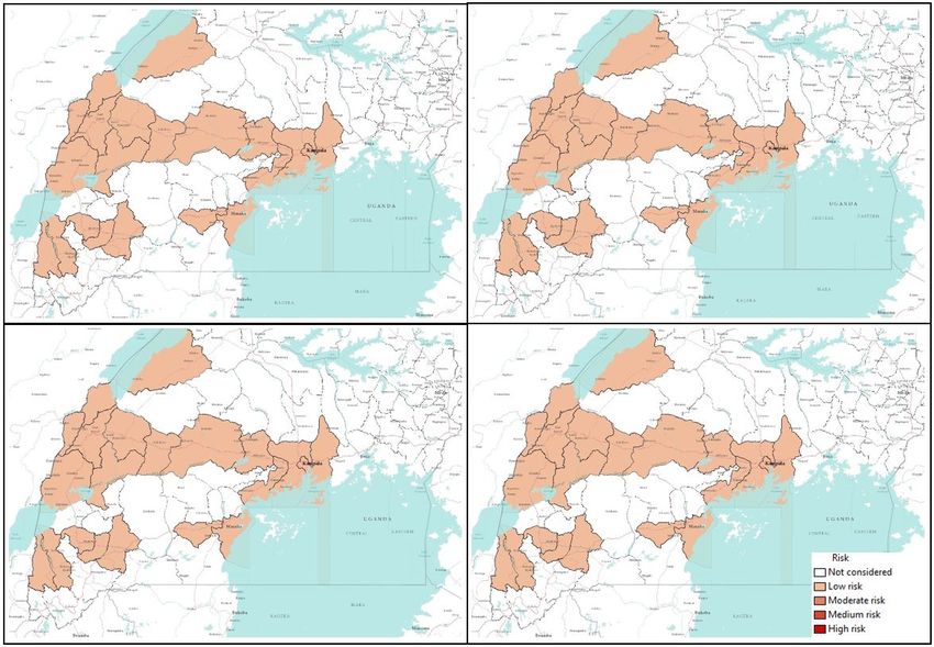
bioRxiv preprint first posted online May. 23, 2019; doi: http://dx.doi.org/10.1101/645598. The copyright holder for this preprint
  (which was not peer-reviewed) is the author/funder, who has granted bioRxiv a license to display the preprint in perpetuity.
                                   It is made available under a CC-BY 4.0 International license.

Risk assessment method
In this section we propose the novel method for risk assessment using multilayer temporal network, Sa Si Ia Ii R spreading
model and the adaptation of Gillespie algorithm for temporal network.

Multilayer temporal network
We consider a population of N individuals connected with two different types of links. These individuals can have links in two
different layers. In the first layer L1 , the links are considered permanent. Therefore, in this layer, contacts among individuals
are not changing. There are potential links in the second layer L2 based on some certain probability distributions. These
potential links/contacts are activated once individuals at the both end of this link are active simultaneously. The activation of
the individuals are driven by a activity rate (γ). The intersection of the two network layers are assumed empty. Once both nodes
are active, the link between them become active with a probability P0 . This probability can have a different value depending on
the nodes the link is connecting. Therefore, this temporal network has the ability to incorporate the heterogeneous contact
probability. However, in this work a single P0 is used in the absence of specific information about the contact between active
node pairs. In the subsequent section of this work, we call L1 as permanent layer while L2 is called temporal/potential layer24 .
The generalized structure of multilayer temporal network is in presented in Figure 1.

Figure 1. A generalized representation of the multilayer temporal model at a specific time t. White circles represents inactive
nodes while red circles represents active nodes. Separate rectangles represent two different layers. Dark solid lines show
permanent links while coloured lines show links in the potential layer. A Potential link becomes active with a probability P0
when both ends of the link are active nodes.

    In the permanent layer, a link can always transmit infection irrespective of its active status while a link in potential layer
transmits the infection only when it connects two active individuals. At a single time step, one node can only be active or
inactive. When a node becomes active, it can come in contact with the active potential active neighbours in L2 and with a
probability P0 , it activates the potential contact. When one of the nodes in the in the contact becomes deactivated, the link

                                                                                                                                     3/20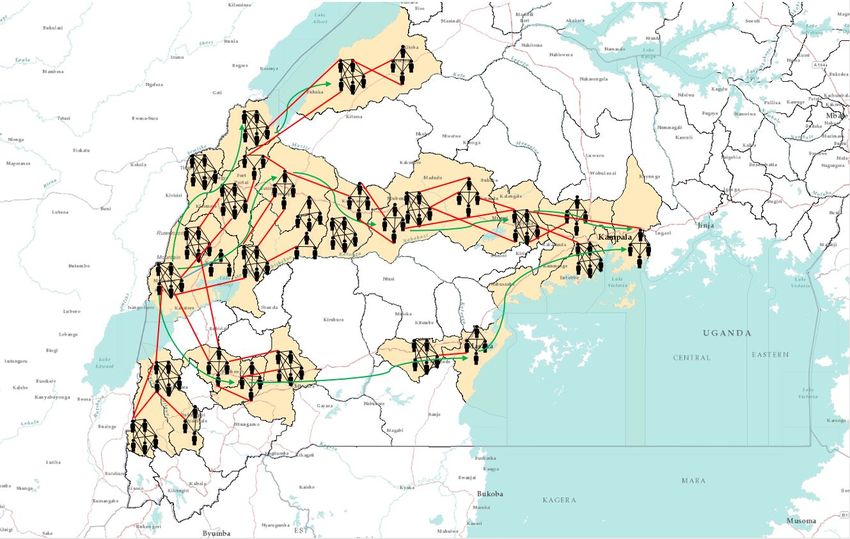
bioRxiv preprint first posted online May. 23, 2019; doi: http://dx.doi.org/10.1101/645598. The copyright holder for this preprint
  (which was not peer-reviewed) is the author/funder, who has granted bioRxiv a license to display the preprint in perpetuity.
                                   It is made available under a CC-BY 4.0 International license.

vanishes and the probability of infection through that link becomes zero again. We assume this process of a node being active or
inactive a Poisson process where a node becomes active and deactivated with rate γ1 and γ2 respectively. Therefore, a node will
stay active for a period of γ2−1 as an active node changes its state with a rate γ2 . Thus we can assume a high value of γ2 and γ1
for a specific node will reflect the reduced duration of the potential link. In this work we assume a similar value for therefore in
the subsequent section, we express γ1 and γ2 as γ only and refer it as activity rate. Therefore, increased γ means an increasing
frequency of a node becoming active and inactive. For example, if we assume an individual becomes active once he starts a
movement/trip and stays active until the trip is finished then a decreased γ means an length of the trip and an increase in the
frequency of this kind of trips. Moreover, if a node does not participate in the occasional contacts —it never becomes active—
γ is set equal to zero for that node. Inactivation times for nodes are exponentially distributed, and therefore the temporal contact
duration has an exponential distribution. In fact, a temporal contact disappears with the inactivity of a node or both in the link24 .
This temporal network is different from the widely used activity driven network in the contact structure among individuals. In
the activity driven network, links are created and destroyed completely randomly and there are no permanent links. In the next
time period, all these links are removed and new links are created with a specific node when it becomes active.

Sa Si Ia Ii R epidemics on multilayer temporal network
In this section, we describe the modification of Susceptible-Infected-Removed (SIR) model for our multilayer temporal network.
SIR model is a popular approach for studying infection spreading where infected people dies or eventually recovers and gains
life-long immunity. For disease such such as Chicken pox, EVD etc., SIR model has the potential to describe the disease
dynamics and infection spreading. In SIR model, each individual is either susceptible, infected, or removed/recovered. We
assume that the infection and recovery processes are independent Poisson processes. A susceptible node becomes infected
with EVD if it comes in contact with an infected person and this transition happens with a rate β . This is called transmission
rate. Once a person becomes infected, he/she stays infected for a certain period of time. This period is called infectious period.
After the infectious period, individuals either recovers/removed from the infection. The rate at which an infected person leaves
the infected state in called recovery/removal rate and it is inverse of the duration of the infection. For our SIR model, the
recovery/removal rate is denoted as δ which has a unit time−1 . So far we have discussed the basic SIR model. However, for our
multilayer temporal network, we have also status of the individuals (active/inactive). Combining our temporal network model
and SIR spreading process, we can have total five states that an individual can occupy. Therefore, we named the model as Sa Si
Ia Ii R model, where compartments are inactive susceptible , active susceptible, inactive infected, active infected and recovered.
     If the probability of node i occupying inactive susceptible, active susceptible, inactive infected, active infected and recovered
in the mean-filed approximation are expressed as S, Sa , I, Ia , and R respectively, then equations for the time evolution can be
expressed as-
                                                           0
                                                         Si = −γ1i Si + γ2i Sai − β ∑ ai1j Si (I j + Iaj )
                                                                                          j
                                              0
                                            Sai = γ1i Si − γ2i Sai − β ∑ ai1j Sai (I j + Iaj ) − P0 β ∑ ai2j Sai Iaj
                                                                              j                         j

                                                    i0
                                                  I = −γ1i I i + γ2i Iai + β ∑ ai1j Si (I j + Iaj ) − δ I i
                                                                                     j
                                        0
                                      Iai = γ1i I i − γ2i Iai + β ∑ ai1j Si (I j + Iaj ) + P0 β ∑ ai2j Sai Iaj − δ Iai
                                                                       j                           j

                                                                           Ri = δ Iai + δ I i
    Where P0 is the probability of a potential link becoming active once both end of the link is active. aikj is the element of
adjacency matrix Ak where k=1 for permanent layer and k=2 for potential layer.

Adaptation of Gillespie Algorithm
Gillespie algorithm has been widely used to simulate stochastic processes for static network (permanent contacts)25–29 and
dynamic/time-varying networks (temporal/potential contacts)24, 30 . However, our multilayer temporal network has both static
and temporal contacts. Therefore, Gillespie algorithm was adapted to the changed network state at every time step retaining
permanent contacts.

    • Initialize the number nodes in the network (N), state transition matrices, maximum number of events and the final time
      for simulation. Find the transition probability Ri for each node at the next time step and Rtot = ∑ j R j , where j = 1, 2, ...N
      and keep track of the status of the nodes (active/inactive)

                                                                                                                                     4/20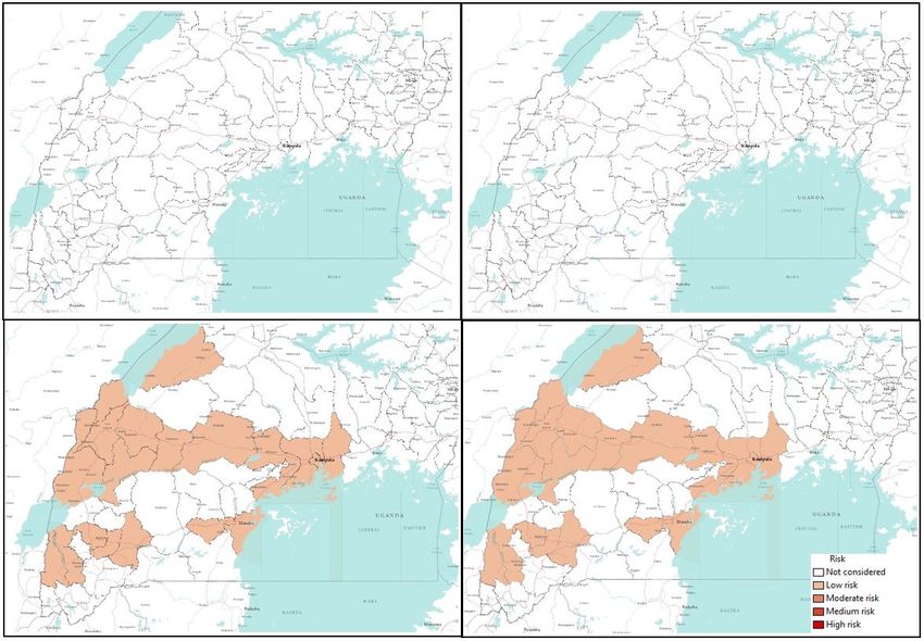
bioRxiv preprint first posted online May. 23, 2019; doi: http://dx.doi.org/10.1101/645598. The copyright holder for this preprint
  (which was not peer-reviewed) is the author/funder, who has granted bioRxiv a license to display the preprint in perpetuity.
                                   It is made available under a CC-BY 4.0 International license.

    • Find the time for the next event which is exponentially distributed with a rate Rtot . The second step is to select a node
      according to the probability distribution Pr(i) = Ri /Rtot which will make a state transition. Later we select a state where
      the transition will happen.
    • Increase the time by time calculated in Step 2. The main difference lies in the update of transition rates for each
      nodes in the network once a transition occurs for our adaptation of Gillespie algorithm. Nodes can change their status
      (active/inactive) as well as changing their states (susceptible, infected, recovered). Therefore, every time a transition
      occurs, the status of the nodes needs to updated and recorded. When a node is in the permanent layer, it’s transition
      probability has the impact of both layer’s neighbours. However, when the node is in temporal layer, it only has the
      impact of its neighbours on the temporal layer. Therefore, the algorithm is modified to account for the network with two
      different layer’s impact on the transition probabilities.
    • Go back to Step 2 unless the stop condition is reached (maximum number of events, the final time for simulation, or
      Rtot < Tolerance).

Calculation of Risk
As the spreading process in our multilayer-based temporal network was highly stochastic, we performed two hundred simulations
for each combination of parameters. We kept track of each node’s status and counted the numbers of simulations in which a
particular node was infected. This count was later used to calculate the risk of EVD spreading in each district. We used the
following formula to calculate the spreading risk to a specific district–
                                                                           Nj
                                                                         ∑n=1 In
                                                             Risk j =
                                                                        Nsimulation
Where, Risk j = Ebola spreading risk of district j, In = Number of simulations where node n is infected, Nsimulation = Number of
simulations, N j = Total number of population in jth district, and j = 1, 2, 3, ...., 23.
   Once we calculate the risk, we can use any mapping software such as ArcGIS software to create risk maps. Risk maps
provide a visual representation of of spreading risks.

Application of Risk assessment for Uganda EVD spreading
We applied our risk assessment method for EVD spreading using generalized movement pattern and a some specific model
parameters. The application of our developed method is presented in this section. First we formulate the multilayer temporal
network for Uganda. Later we used the network with Sa Si Ia Ii R model and the modified Gillespie algorithm to track number
of infected human after a certain period of time and assess the risk of EVD spreading to different spatial location. Simulation
results and discussion are presented for specific scenarios are presented at the end of this section.

Multilayer temporal network for Uganda
We have proposed a multilayer temporal network for Ebola spreading in Uganda. The recent Ebola outbreak in Democratic
Republic of Congo created a possibility of EVD infection in Uganda. We have created a network based on the people’s
movement for different purposes such as fish trade, cattle trade and general movement for different purposes. The movement
pattern and districts in the movement paths are obtained from confidential data provided by Ministry of Health, Uganda. These
data are then used to formulate an example of human movement network for some selected districts in Uganda. We have
observed the focus of Ebola preparedness by the Ministry of Health and partners to select possible point of entry for Ebola
patient from DRC. We found out that Kasese district is at the high risk of EVD infected person’s entry point. Therefore we
choose this district as our point of entry. Once an infected person from DRC enters into Uganda through the bordering districts,
they come in contact with susceptible people in that location. Now, Ebola being highly contagious, infected person/persons can
spread the infection to people they come in contact with. People moves from one location to another for different reasons and
there is always a pattern for this movement. For Uganda, we have obtained some general information about the local peoples
movement pattern and incorporate them in our multilayer network. People movement from one location to another are mostly
motivated by several reasons. For Uganda, we found out that these movements are mostly for three different purposes. They are
following-

   1. Fish trade towards southward direction from the point of entry
   2. General movement for daily commute, shopping, visiting relatives, search of work, or travelling for various purposes.
      These types of movement starts in the point of entry in the bordering districts and goes all the way to capital city Kampala.
      People mostly travels from rural areas to neighbouring big cities. Once they come in contact with other people there and

                                                                                                                                     5/20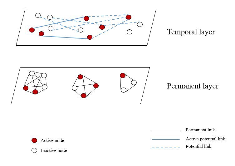
bioRxiv preprint first posted online May. 23, 2019; doi: http://dx.doi.org/10.1101/645598. The copyright holder for this preprint
  (which was not peer-reviewed) is the author/funder, who has granted bioRxiv a license to display the preprint in perpetuity.
                                   It is made available under a CC-BY 4.0 International license.

       this results in a certain mixing among individuals from locations. This mixing happens throughout this movement path.
       There are several of this movement paths which are presented in the Figure 2 with green arrows.

   3. Limited movements due to cattle trade. The movements for cattle trade are mostly local or between neighbouring districts.
      long distance cattle trade happens in commercial scale and does not include much movement of people as they happens
      mostly via organized transportation system.

    To represent this contact structure and movements in Uganda, we propose a multilayer contact network. We create a specific
network for human movement from Kasese to Kampala based on general movement information. The network is used to show
an example of the developed method for risk assessment. As we have described in our Temporal network section, we assumed
two layers in the network. The permanent layer consists of the contacts of each individuals within each household. Each family
in Uganda has an average of 6 children31 . Therefore, with the parents we can assume around 8 people in a household in average.
We assume a distribution of population where each household can have 5-10 members.
    Within each household, we can assume permanent links among family members. Therefore, links within each household
can construct the permanent layer in the Uganda network for Ebola spreading. The potential layer can be formed incorporating
individuals movement for different purposes. An individual becomes active once it is in the movement and stays active until it
finishes its movement. Once a node is in movement (active), its potential links with individuals other than own family can be
activated based on the active status of the other nodes that has link with our specific node. This can be explained as following-
node i has potential links with a set of node named J throughout the whole network. Therefore, once node i is active, potential
links with any of the node in J can be activated if that node itself is active as well. This link activation structure is very crucial
in the proper representation of the contact structure. As both of these node are in movement, they can come in contact with
each other in different places such as transportation, marketplace, visiting sites etc. Usually the movement pattern between
individuals follow a general structure. Within each location, there is a probability that individuals will come in contact with
each other for various purposes. Inter-location contacts also follow some structure rather than being completely randomized.
People usually flock into big cities or towns nearby where they will come in contact with the local active people or others
coming in to that location for similar purposes. When this happen, if two of these active individuals have a potential link, that
will be activated and there will be a possibility of infection via that link.
    Districts we have used in our Uganda network are presented in Table 1. We have used the centroid of each district to find
the distance between two districts while formulating the network. However, this is one realization of the network built using
available movement data. Some Ugandan districts are not included in our assessment, therefore there may have been districts at
high risk that are excluded from the risk assessment performed in this article. We have scaled the population in each district by
1000 in our network for computational purposes. As our main purpose is to evaluate the risk of EVD, this scaling has greatly
reduced the computational complexity. We have incorporated in the network all previously discussed movement patterns along
different paths from one point of entry to Kampala. These movements and their directions are also shown in Figure 2. We
have considered all districts that are in movements paths of any nature towards Kampala from Kasese. Although all bordering
districts are at risk of Ebola introduction, we focus on demonstrating the application of our method when the initial infections
are in the Kasese district.
    In summary, our network for Ebola spreading in Uganda consists of 23 districts where permanent layer incorporates the
contacts among individuals within a household. Potential layer reflects the contacts between individuals which can happen only
when both ends of the link are active due to some kind of movement and they have a possibility of pathogen transfer between
them.

Simulation Setup
Upon formulation of the multilayer network, we perform simulations with the Si Ia Ii R model for EVD spreading using Gillespie
algorithm24, 32 . The network is temporal as depending on the active status of nodes, links are changing in the potential layer. We
conduct our simulation with two major goals— observe the progression of EVD spreading with time throughout the network
and evaluate the risk of spatial spreading for this specific scenario.
    In our temporal simulations, we have four different parameters. They are the rate at which individuals become active
and inactive (γ1 and γ2 , generally we will call them activity rate γ as both of them have same value for our simulations), the
transmission rate β , the recovery rate δ , and the probability P0 of pathogen transmission via a potential link between two
simultaneously active individuals in the potential layer. These values are hard to estimate and due to high stochasticity in
the people’s movement pattern, movement parameters i.e. (γ) can not be expressed with a single value. The transmission
rate β is also variable and takes different values for different outbreaks depending on the contact pattern among individuals.
Therefore, we perform simulations with multiple values of each parameter to explore the sensitivity of the epidemic size and
and spreading risk to different districts from the initial outbreak location. For each parameter set, we calculate total number of
infected individuals with time and create risk map.

                                                                                                                                     6/20
bioRxiv preprint first posted online May. 23, 2019; doi: http://dx.doi.org/10.1101/645598. The copyright holder for this preprint
  (which was not peer-reviewed) is the author/funder, who has granted bioRxiv a license to display the preprint in perpetuity.
                                   It is made available under a CC-BY 4.0 International license.

Figure 2. Multilayer temporal network for EVD spreading in Uganda. The districts considered for our network model are
coloured in baize (23 districts). Small human shapes represents individual human beings. This figure does not represent the
actual network, rather it is a visual representation of the multilayer network. Each cluster of human represents a households and
black lines among them represents permanents contacts. Red lines represent contacts in potential layer. These links only
become active when both individuals in the link are active simultaneously. A link represents a possibility of pathogen
transmission. Green directional arrow represents the directions of human movements.

    We present the number of infected individuals in each time step for each parameter set. As we have multiple parameters, we
choose the value of P0 =0.7 and 0.1 which represents the seventy percent and ten percent chance of the pathogen transmission
via a potential link between two active nodes. For the value of rate a node becomes active and inactive, we choose γ= 0.1 and
0.5. This can be explained as following, a particular individual becomes active in every 1γ days and once active, it stays active
for next 1γ days. For example, γ= 0.1 represents the frequency of a node being changing its state (inactive to active, active to
inactive) in every 10 days.
    The value of the transmission rate is mostly estimated from the real incidence data in most of the literature where Ebola
model is fit to the past incidence data. For our work, we are more interested in the risk assessment and provide different
scenarios under different human movement and weather conditions. Therefore, a range of parameter values are used to quantify
the size of the epidemic and assess the risk of EVD spreading to different locations from the initial outbreak location in Uganda.

Results and Discussion
We initiated our simulation with a single active infected person in Kasese district and tracked the status of each node in the
network for a period of 150 days to see how each node is changing their status (active susceptible, inactive susceptible, active
infected, inactive infected, and recovered). At the end of the simulation time (150 days), total number of infected people in the
outbreak are calculated and the risk of a specific node being infected during the outbreak was assessed.
    To measure the progression and the severity of Ebola spreading, we track total number of infected and cumulative number
of infected people for a period of 150 days. For any infection spreading, some important measures are the size of the peak
infection (maximum number of simultaneously infected individuals), time to reach that peak and total number of infected
within an outbreak (epidemic size)29 . Therefore, we designed our simulation to keep track of both the number of infected and

                                                                                                                                     7/20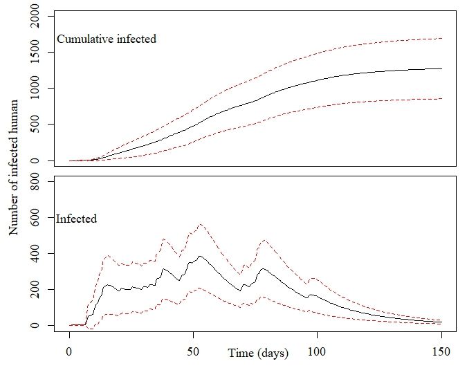
bioRxiv preprint first posted online May. 23, 2019; doi: http://dx.doi.org/10.1101/645598. The copyright holder for this preprint
  (which was not peer-reviewed) is the author/funder, who has granted bioRxiv a license to display the preprint in perpetuity.
                                   It is made available under a CC-BY 4.0 International license.

                                                        Districts          Population
                                                        Bundibugyo         224387
                                                        Bunyangabu         181200
                                                        Bushenyi           234440
                                                        Hoima              572986
                                                        Kabarole           469236
                                                        Kampala            1507080
                                                        Kamwenge           414454
                                                        Kanungu            252144
                                                        Kassanda           100038
                                                        Kasese             694992
                                                        Kyegegwa           159800
                                                        Kyenjojo           422204
                                                        Lwengo             267300
                                                        Masaka             297004
                                                        Mbarara            472629
                                                        Mityana            328964
                                                        Mpigi              250548
                                                        Mubende            684337
                                                        Mukono             594804
                                                        Ntorko             70900
                                                        Rukungiri          314694
                                                        Sheema             180200
                                                        Wakiso             1997418

                             Table 1. Districts considered in our Uganda multilayer temporal network

cumulative number of infected at each time step of 150 days simulation period. Our simulation results are presented in the
subsequent part of this section. We have chosen values of transmission rate β to explore varying range of transmission potential
given a contact with infected individual. We have presented simulation results for β =0.2, 0.5, 1.7, 2.5 in the results section.
     Figure 3 represents the number of cumulative infected and infected humans for P0 =0.7 and γ=0.5 and a varying range of
transmission rate β .
     Within each sub-figure in Figure 3, the top graph represents the cumulative number of infected while the bottom plot
represents number of simultaneously infected humans at different time steps.
     From Figure 3 (P0 =0.7 and γ=0.5), it is evident that with the increase of β , the infection size increases rapidly. An increase
of β from 0.2 to 0.5 increases the infection size from 2459 to 6634. Therefore, very small increase in the transmission causes a
huge increase in the total number people infected with Ebola when we assume a 70% chance of pathogen transmission once an
active infected individual comes in contact with another active susceptible person in the potential layer. Also, in this simulation
set, the potential layer assumed to be highly active/mobile as people assumed to become active and inactive within a period of
two days.
     The number of simultaneously infected people at a certain time is very important for public health personnel33 . More
infected people means preparation of more hospital beds, doctors and medical supplies34 . Therefore, once a outbreak occurs, it
is very important to have an idea about the maximum number of simultaneously infected people (size of the peak infection)29 .
In each of the sub-figure, the bottom plot shows simultaneously infected people at each time step. In the plot, the peak infection
size also increases with β . However, when β =0.2, the peak is not very pronounced and peak infection size is around 600.
However, for other values of β , The peak is more pronounced and the peak infection size is more than 2500 for all other values
of β . The time to reach the peak for for β =0.2 is around 50 days. With the increase of β , the the infection plot becomes skewer
to the left, meaning faster arrival to the peak infection size. Therefore, faster arrival to peak infection and greater value of
peak infection size indicates a widespread epidemic outbreak. Therefore, simulations for this specific parameter set indicates a
widespread and severe outbreak for for β >0.5 where more than 50% of our total population in the network becomes infected.
     For each parameter set, we have estimated the risk of EVD spreading to different spatial location when we start the infection
at Kassese district with a single infected individual. We have created risk maps using ArcGIS for the spreading of Ebola to
distant locations. We have used equation for Risk explained the "Material and Methods" section to calculate the risk. Value of
the risk is classifies in 5 different categories as presented in Table 1.

                                                                                                                                     8/20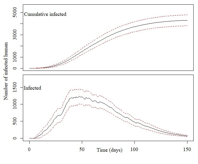
bioRxiv preprint first posted online May. 23, 2019; doi: http://dx.doi.org/10.1101/645598. The copyright holder for this preprint
  (which was not peer-reviewed) is the author/funder, who has granted bioRxiv a license to display the preprint in perpetuity.
                                   It is made available under a CC-BY 4.0 International license.

                              (a) β =0.2                                                                 (b) β =0.5

                             (c) β =1.7                                                                 (d) β =2.5

Figure 3. Number of cumulative infected and infected individuals in the Uganda Ebola network with 95% confidence interval for P0 =0.7,
γ=0.5, and, (a) β =0.2 , (b) β = 0.5 , (c) β =1.7, and (d) β = 2.5

                                                                                                                                     9/20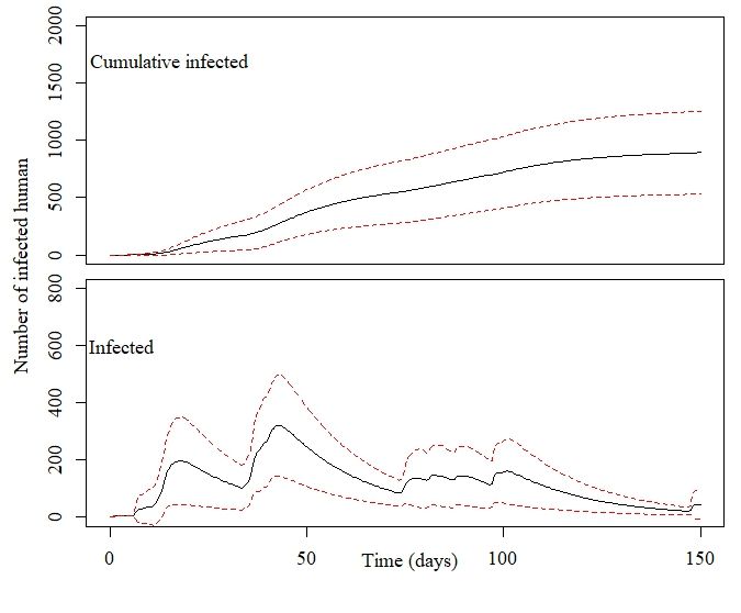
bioRxiv preprint first posted online May. 23, 2019; doi: http://dx.doi.org/10.1101/645598. The copyright holder for this preprint
  (which was not peer-reviewed) is the author/funder, who has granted bioRxiv a license to display the preprint in perpetuity.
                                   It is made available under a CC-BY 4.0 International license.

                                          Risk                             Value of risk parameter
                                          No risk or not considered        0
                                          Low risk                         0 < risk ≤ 0.2
                                          Moderate risk                    0.2 < risk ≤ 0.4
                                          Medium risk                      0.4 < risk ≤ 0.6
                                          High risk                        > 0.6

                  Table 2. Classification of risk for our spatial locations based on the value of risk parameter.

    Risk maps in Figures 4, 6, 8, and 10 show all the neighboring districts in the south part of Uganda although we have
considered only 23 districts, which are considered being in the path of people’s movement network from Kasese to Kampala.
Therefore, there are some districts in the maps that have not been considered in our multilayer temporal network and hence
have not been assessed for risk.
    Figure 4 shows a risk map for four selected values of β and P0 = 0.7 and γ = 0.5. The map is coloured with a monochromatic
colour gradient which increases with increase of risk. Therefore, districts which are white in the map are either not at risk (if
considered in the network model) or not considered in the network model.

Figure 4. Risk map of Ebola spreading within selected 23 districts in Uganda for β =0.2 (top left), 0.5 (top right), 1.7 (bottom
left), 2.5 (bottom right). The map is colour coded according to the risk of Ebola spreading.

    From the risk map for β =0.2 in Figure 4, we can see that all our selected locations are at low risk or moderate risk as
the transmission rate is very low. However, some of the districts are at comparatively high risk than others. For this specific
scenario with β =0.2, Bundibugyo, Bushenyi, Kyegegwa, Kyenjojo, Masaka, Mpigi, and Sheema districts are at higher risk than
other districts in our network. However, aforementioned districts are at moderate risk of Ebola spreading while other districts
are at low risk for β =0.2. Increasing the value of β increases the risks proportionately which can be seen from Figure 4. The

                                                                                                                                     10/20
bioRxiv preprint first posted online May. 23, 2019; doi: http://dx.doi.org/10.1101/645598. The copyright holder for this preprint
(which was not peer-reviewed) is the author/funder, who has granted bioRxiv a license to display the preprint in perpetuity.
It is made available under a CC-BY 4.0 International license.
colour gradients are increasing in the risk maps with the increasing β . In the risk maps for other values of β , a similarity in the
risk is observed. This is evident from similar colour gradient of districts in all three maps for β =0.5, 1.7, and 2.5, which can be
explained from similar epidemic size and comparable infection peaks for these values of β (Figure 3). Therefore, we have a
similar infection spreading in these cases and assessed risks are similar (not same , but they are in the same interval presented
in Table 1). There was an increasing trend in the value of calculated risk parameters with the increase of β , although in the
map they are included in the same interval. Districts in the temporal network for β = 0.5, 1.7 and 2.5 with assessed risks are
presented in Table 2.
Risk Districts
High risk Bundibugyo, Bunyangabu, Bushenyi, Kanungu, Kyegegwa, Kyenjojo, Lwengo, Masaka, Mpigi, Sheema
Medium Risk Hoima, Kasese, Mbarara, Mityana, Mubende, Ntoroko, Rukungiri, Kassanda
Moderate risk Kampala, Kamwenge, Wakiso
Low risk Kabarole, Mukono
Table 3. Districts in the network and their associated risk for EVD spreading
Table 3 shows that 10 of 23 districts are at high risk of EVD spreading in case of an outbreak. With current outbreak in
DRC, it is expected that bordering districts will be at high risk of EVD spreading. However, our simulation results has the
capability to incorporate the movement data that shows non-bordering districts can also be at high risk due to infected person’s
movement. This is can be easily seen from Figure 4, where some non-bordering districts demonstrates high or medium risk of
EVD spreading.
Figure 5 represents the number of infected individuals for P0 =0.7 and γ=0.1. γ = 0.1 means individuals have the probability
of becoming active and inactive in every 10 days. Therefore, decreasing the γ decrease the probability of a human becoming
active while increasing the time of him/her staying active.
The peak infection increases from 450 to 1700 for our selected values of β =0.2 to 2.5 while the cumulative number of
infected increases from 1607 to 59.
Comparing the simulation results in Figure 3 and 5 for similar value of β , the epidemic size as well as the peak infection is
always higher for higher values of γ. Higher value of γ can be translated to the increased human movement in our network. As
we are assuming that a human is active when it is in a movement, a higher γ for a person means frequent short trips while lower
γ means longer trips which are not very frequent.
Higher γ increases the time a human will be in the active (mobile) state, While lower value indicates longer length of an
individual staying active24 . Therefore, it is convenient to assume that while an infected individual is active for a longer period
of time, it will eventually spread the infection to more active individuals in the potential layer35 . However, our simulation
results show otherwise. An increase in the value of γ increases the infection size as well as the peak infection size (Figure 3 and
Figure 5).
Therefore, our simulation results show the frequency at which individuals become active or inactive dominates over the
time span of the individual staying active. This is evident from the higher size of the epidemic from the higher value of γ.
For β =0.2, the cumulative number of infected after 1607 when it is 59 when we have γ=0.5. The value of the cumulative
number of infected is also higher for other cases as well. The infection reaches to the peak infection slowly (approximately 50
days) irrespective of the value of the transmission rate. Therefore, lower value of the activity rate γ means lesser number of
simultaneously infected people and slow infection spreading within the spatial locations (Figure 4 and Figure 6). As we have
discussed earlier, lower value of γ reflects the reduced movement of people. Therefore, from the comparison of simulation
results in Figure 3 and Figure 5, it is evident that human movements are critical in the severity and speed of EVD spreading. As
frequent human movements (frequent short trips) spreads the EVD very fast, reduced human movement may minimize the
severity of the EVD spread36 . This is also evident from the risk map showed in Figure 6 for reduced γ. From the map, we can
see that Bundibugiyo, Sheema and Masaka are three districts which are most at risk of Ebola spreading for our specific network
model. For these three districts, the risk of spreading is comparatively higher than other districts even when the value of the
transmission rate is very low. For example, these districts are in moderate risk zone while others in low risk zone for β =0.2.
However, with the increase of β , the value increases and for our highest value of β =2.5, these three districts are at the highest
risk of Ebola spreading. Table 3 presents districts in the temporal network for β = 2.5 with assessed risks.
During the network creation, some of the districts were assumed to be possible mixing places, which makes them more
vulnerable than others. Therefore, simulation results and evaluated risks are obtained according to the network structure. An
example of dependency on the network structure is evident from Figures 4 and 6, showing the district of Kabarole at a low risk
for all values of β , despite being a bordering district to DRC. This low risk for Kabarole can be attributed to the fact that this
district was not considered as a mixing place in our network. This demonstrates our method’s adaptability to specific data about
each locations in the network.
11/20bioRxiv preprint first posted online May. 23, 2019; doi: http://dx.doi.org/10.1101/645598. The copyright holder for this preprint
(which was not peer-reviewed) is the author/funder, who has granted bioRxiv a license to display the preprint in perpetuity.
It is made available under a CC-BY 4.0 International license.
(a) β =0.2 (b) β =0.5
(c) β =1.7 (d) β =2.5
Figure 5. Number of infected individuals in the Uganda Ebola network with 95% confidence interval with P0 =0.7, γ=0.1, and for (a)
β =0.2 , (b) β =0.5 , (c) β =1.7, and (d) β = 2.5
Risk Districts
High risk Bundibugyo, Masaka, Sheema
Medium Risk Bunyangabu, Bushenyi, Hoima, Mbarara, Mityana, Mpigi, Kyegegwa, Kyenjojo, Lwengo, Kanungu
Moderate risk Kampala, Kamwenge, Wakiso, Rukungiri, Ntoroko, Mubende, Mityana, Kasese, Kassanda
Low risk Kabarole, Mukono
Table 4. Districts in the network and their associated risk for Ebola spreading for P0 =0.7, γ=0.1 and β =2.5
12/20bioRxiv preprint first posted online May. 23, 2019; doi: http://dx.doi.org/10.1101/645598. The copyright holder for this preprint
(which was not peer-reviewed) is the author/funder, who has granted bioRxiv a license to display the preprint in perpetuity.
It is made available under a CC-BY 4.0 International license.
Figure 6. Risk map of Ebola spreading within selected 23 districts in Uganda for β =0.2 (top left), 0.5 (top right), 1.7 (bottom
left), 2.5 (bottom right). The map is colour coded according to the risk of Ebola spreading.
Comparing table 2 and Table 3, it is evident that when we have a lower γ, risks decreases significantly. For same values of
β , lower γ reduce the risk of Ebola spreading. When β ≥ 0.5 and γ=0.5, there are eleven high risk districts. Decreasing the
value of γ to 0.1 results in only 3 high risk districts for β =2.5. For other values of β and γ=0.1, none of the districts in our
network model are at high risk. Therefore, reducing human movements has shown significant decrease in the Ebola spreading.
However, reducing human movement is not practical as human movements can not be controlled. Therefore, we focus on
the parameter P0 which express the possibility of pathogen transfer via an active potential link. P0 can be expressed as the
probability of an active infected person spreading the virus to an active susceptible person. The value of this parameter is
dependent on direct physical contact between infected and susceptible. In our previous set of simulations, we used P0 =0.7 in
our previous simulations. Now if we can decrease the possibility of the physical contacts among humans in case of an outbreak,
it would be equivalent to a reduced possibility of virus transfer. To observe the impact of reduced physical contact i.e. lower P0 ,
we conducted simulation for a P0 =0.1 reflecting only 10% possibility of pathogen transfer via an active link while one of the
human is infected. Simulations results for P0 =0.1 are presented in Figures 6-9.
Decreasing the probability of Ebola spreading (i.e. P0 ) to 10% from 70% via a contact in potential layer significantly
reduces the infection size as well as simultaneously infected humans. However, while changing the P0 , similar values of γ are
used as before.
Figure 7 shows cumulative infected and infected humans for γ=0.5 and P0 =0.1. For our lowest value of β =0.2, cumulative
number of infected human are 45 after 150 days. Increasing β increased the value of cumulative infected humans to 1274 for
β =2.5. Therefore, number of cumulative infected humans are very low compared to cumulative infected humans for similar
values of β with P0 =0.7. Also there is no pronounced single peak while maximum simultaneously infected people goes around
400 for the highest used value of β . Therefore, decreasing P0 reduces number of infected humans and therefor the severity of
EVD spreading.
Figure 8 shows risk maps for P0 = 0.1 and γ = 0.5. It is evident from the map that, all districts in our network are at low risk
13/20bioRxiv preprint first posted online May. 23, 2019; doi: http://dx.doi.org/10.1101/645598. The copyright holder for this preprint
(which was not peer-reviewed) is the author/funder, who has granted bioRxiv a license to display the preprint in perpetuity.
It is made available under a CC-BY 4.0 International license.
(a) β =0.2 (b) β =0.5
(c) β =1.7 (d) β =2.5
Figure 7. Number of infected individuals in the Uganda Ebola network with 95% confidence interval with P0 =0.1, γ=0.5, and for (a)
β =0.2 , (b) β =0.5 , (c) β =1.7, and (d) β = 2.5
14/20bioRxiv preprint first posted online May. 23, 2019; doi: http://dx.doi.org/10.1101/645598. The copyright holder for this preprint
(which was not peer-reviewed) is the author/funder, who has granted bioRxiv a license to display the preprint in perpetuity.
It is made available under a CC-BY 4.0 International license.
Figure 8. Risk map of Ebola spreading within selected 23 districts in Uganda for β =0.2 (top left), 0.5 (top right), 1.7 (bottom
left), 2.5 (bottom right). The map is colour coded according to the risk of Ebola spreading.
15/20bioRxiv preprint first posted online May. 23, 2019; doi: http://dx.doi.org/10.1101/645598. The copyright holder for this preprint
(which was not peer-reviewed) is the author/funder, who has granted bioRxiv a license to display the preprint in perpetuity.
It is made available under a CC-BY 4.0 International license.
for EVD spreading for selected values of β .
Further decreasing the value of γ to 0.1 decreases cumulative number of infected humans as well as peak infection size.
Figure 9 shows that, when β is 0.2 and 0.5, the EVD does not spread at all and stays within the outbreak location with only
2-3 infected persons. However, increasing the value of β increases number of infected humans but the cumulative number of
infected remains less than 150 even for our highest value of transmission rate (β = 2.5).
(a) β =0.2 (b) β =0.5
(c) β =1.7 (d) β =2.5
Figure 9. Number of infected individuals in the Uganda Ebola network with 95% confidence interval with P0 =0.1, γ=0.1, and for (a)
β =0.2 , (b) β = 0.5 , (c) β =1.7, and (d) β = 2.5
Figure 10 shows no risk of EVD spreading for β =0.2 and 0.5. However, with increasing β , all our districts are at low risk
of EVD spreading.
Summarizing simulation results and risk maps presented in Figures 6-9, we can see a significant reduction in the epidemic
size and simultaneously infected humans when P0 =0.1. Therefore, a reduction in probability of pathogen transfer via a potential
link i.e. reduced physical contact between humans while they are active/mobile greatly reduce the number of infected as well as
severity of EVD. It also reduces the risk of EVD spreading.
EVD spread from physical contact with bodily fluid such as blood, feces, vomit, saliva, mucus, tears, breast milk, urine,
semen, sweat etc from infected persons. Therefore, a susceptible person can only be infected with EVD if it comes in contact
16/20bioRxiv preprint first posted online May. 23, 2019; doi: http://dx.doi.org/10.1101/645598. The copyright holder for this preprint
(which was not peer-reviewed) is the author/funder, who has granted bioRxiv a license to display the preprint in perpetuity.
It is made available under a CC-BY 4.0 International license.
Figure 10. Risk map of Ebola spreading within selected 23 districts in Uganda for β =0.2 (top left), 0.5 (top right), 1.7
(bottom left), 2.5 (bottom right). The map is colour coded according to the risk of Ebola spreading.
17/20bioRxiv preprint first posted online May. 23, 2019; doi: http://dx.doi.org/10.1101/645598. The copyright holder for this preprint
(which was not peer-reviewed) is the author/funder, who has granted bioRxiv a license to display the preprint in perpetuity.
It is made available under a CC-BY 4.0 International license.
with these bodily fluids from an infected human. Therefore, if infected people are identified and moved to quarantine and
restrict to travel, then the infection can be contained. However, non-hospitalized people during early symptomatic stage keep
moving for their daily life and spread the infection with people they come in contact with. Early detection in countries where
people are not very health conscious is very challenging. Therefore, when an infected case is found, if human movements are
reduced significantly, the spread can be contained. Our simulation results conform with this movement reduction and reduced
EVD infected cases. However, this not practical as human movements can not be controlled.
Activity rate (γ) can be translated to human movements within the network, therefore increasing activity rate means
increased but shorter duration human movements. From all simulation results, it is evident that an increase in activity rate
increases the epidemic size and as well as the speed of the infection to reach its peak. Therefore, increasing activity rate means
a severe and fast EVD spreading. Simulation results suggest that, short duration but frequent human movements result in
greater number of infected humans and high risk of EVD spreading than longer duration but less frequent movements.
The probability at which infection spreads to susceptible people via a potential contact (P0 ) has obvious impacts on the
epidemic size. Increasing P0 increases the epidemic size irrespective of the activity rate γ which is evident from Figures 2,4,6,
and 8. Comparing Figure 3 and Figure 7 as well as Figure 5 and Figure 9, for similar values of the activity rate, decreasing P0
decreases the number of infected humans significantly. P0 can be translated to the probability of physical contact of infected
mobile humans with others. Therefore, our simulation results conforms with another mitigation strategy against EVD spreading
which is to stay away from contact with people whose status with respect to EVD are not know. The lower value of P0 can be
achieved by minimizing physical contact among people during movements/travels. If people are aware of the risk of EVD
spreading in their area and keep themselves from physical contact with others, it will significantly reduce infected cases in case
of an outbreak.
Risk maps shows that there some districts as shown in Table 2 and 3, who are at higher risk of Ebola spreading in our
network for our specific network scenario. The risk assessment provides an important information for Ebola preparedness.
Ebola preparedness includes setting up medical facilities as well as employing different preventive measures for Ebola spreading.
However, resources are limited and it is always essential to find a way utilize the resources in a fruitful way. However, our risk
only showed examples of of our developed risk assessment method where we have used very limited generalized movement
data. Although proposed risk assessment method have the capability to provide guidelines for public health people, it requires
more accurate movement data to be used practically in the field. Future work will include an evaluation of the impact of major
EVD intervention pillars (i. e., coordination, vaccination, surveillance, risk communication, case management, and safe burials)
on the risk assessment, to provide a realistic picture under multiple scenarios.
Conclusions
We present a novel method for risk assessment based on a multilayer temporal network. This method has the ability to assess
risk of EVD spreading when accurate network data is available and can be a important tool for public health people during an
outbreak. We demonstrate an application of our developed method using a multilayer temporal network formulated with generic
and incomplete movement data in Uganda. Simulations results from this multilayer temporal network confirm that reduced
physical contacts with people while travelling, and taking other preventive measures decrease the risk of EVD spreading.
Simulations also show that some districts are at higher risk than others in the considered scenario. This provides public
health personnel directions about prioritizing their effort to limit EVD spreading during an outbreak. However, assessed risks
are crucially dependent the network structure and can be fully trusted for resource allocation once accurate individual-level
movement data in time and space are available.
References
1. Dixon, M. G. & Schafer, I. J. Ebola viral disease outbreak—west africa, 2014. MMWR. Morb. mortality weekly report 63,
548 (2014).
2. World health Organization. Ebola virus disease (2018). https://www.who.int/news-room/fact-sheets/detail/
ebola-virus-disease, Last accessed on 2019-04-22.
3. CDC: Centers for Disease Control and Prevention. Ebola outbreak in eastern democratic republic of congo tops 1,000
cases (2019). https://www.cdc.gov/media/releases/2019/s0322-ebola-congo.html, Last accessed on 2019-04-22.
4. Ajelli, M. et al. Comparing large-scale computational approaches to epidemic modeling: agent-based versus structured
metapopulation models. BMC infectious diseases 10, 190 (2010).
5. Potterat, J. J. et al. Sexual network structure as an indicator of epidemic phase. Sex. transmitted infections 78, i152–i158
(2002).
6. Rizzo, A., Pedalino, B. & Porfiri, M. A network model for ebola spreading. J. theoretical biology 394, 212–222 (2016).
18/20You can also read