Robustness of topological defects in discrete domains
←
→
Page content transcription
If your browser does not render page correctly, please read the page content below
PHYSICAL REVIEW E 103, 012602 (2021)

                                   Robustness of topological defects in discrete domains
                                                                       *                           †
                                               Karl B. Hoffmann            and Ivo F. Sbalzarini
                               Technische Universität Dresden, Faculty of Computer Science, Dresden, Germany;
                               Max Planck Institute of Molecular Cell Biology and Genetics, Dresden, Germany;
                                           Center for Systems Biology Dresden, Dresden, Germany;
                                       and Cluster of Excellence Physics of Life, TU Dresden, Germany

                   (Received 1 October 2020; revised 30 November 2020; accepted 2 December 2020; published 5 January 2021)

                   Topological defects are singular points in vector fields, important in applications ranging from fingerprint
                detection to liquid crystals to biomedical imaging. In discretized vector fields, topological defects and their
                topological charge are identified by finite differences or finite-step paths around the tentative defect. As the
                topological charge is (half) integer, it cannot depend continuously on each input vector in a discrete domain.
                Instead, it switches discontinuously when vectors change beyond a certain amount, making the analysis of
                topological defects error prone in noisy data. We improve existing methods for the identification of topological
                defects by proposing a robustness measure for (i) the location of a defect, (ii) the existence of topological defects
                and the total topological charge within a given area, (iii) the annihilation of a defect pair, and (iv) the formation
                of a defect pair. Based on the proposed robustness measure, we show that topological defects in discrete domains
                can be identified with optimal trade-off between localization precision and robustness. The proposed robustness
                measure enables uncertainty quantification for topological defects in noisy discretized nematic fields (orientation
                fields) and polar fields (vector fields).

                DOI: 10.1103/PhysRevE.103.012602

                        I. INTRODUCTION                                       as convolutional filters [1]. This includes differential expres-
                                                                              sions of “diffusive [topological] charge” [19,20] represented
   A topological defect (TD) is a singular point in a polar or
                                                                              by finite-difference stencils and machine learning approaches
nematic vector field. Such fields are ubiquitous in science,
                                                                              using convolutional neural networks [21]. Alternatively, TDs
engineering, and mathematics as coarse-grained continuous
                                                                              and their charge are identified as zeros or close-to-zeros of the
descriptors of flows, force fields, molecule and object orienta-
                                                                              nematic order parameter or a derived quantity [14,22–25].
tion, anisotropy, etc. Therefore, TDs are investigated in a wide
                                                                                 The identified TDs and their charges are discrete quantities
range of applications, including fingerprint alignment [1,2],
                                                                              that cannot depend on each of the input vectors in the discrete
cosmology [3], topological insulators, superconductors, and
                                                                              neighborhood in a globally continuous manner. Hence, even
superfluidity [4]. They also play a central role in the theory
                                                                              smooth vector field dynamics implies discontinuous dynamics
of hard and soft matter [5–7], including active matter [8],
                                                                              of the TDs [9]. Additionally, nematic and polar vectors in
where they are related to active stress [9–12] and to geometric
                                                                              simulation or measurement data are usually subject to uncer-
properties such as curvature [13–16].
                                                                              tainty [15,26–28]. To improve defect identification, previous
   Although TDs are subject to global constraints, like the
                                                                              works therefore used vector field smoothing [e.g., 14,16,29],
Euler characteristic of closed surfaces, they are defined and
                                                                              defect identification along larger fixed-size closed paths [17],
identifiable purely locally. This local identifiability is par-
                                                                              clustering [30], filtering by temporal persistence [29], ma-
ticularly useful in discrete domains, as they occur in digital
                                                                              chine learning [21,25], or thresholds on the nematic order
data, such as numerically solved fields or measurement data
                                                                              parameter, either absolute [14,15] or relative to the spatial
including images. In discrete domains, a TD can be identified
                                                                              mean [22]. While all of these methods work in practice, none
from a finite neighborhood of discretization points.
                                                                              of them are based on a rigorous definition of robustness of
   These neighborhoods are commonly defined by small,
                                                                              TDs, and they do not shed light onto the connection between
fixed-size stencils [17] or wedges [18], or they are expressed
                                                                              the robustness of TDs and the geometry of the underlying
                                                                              vector field.
 *
     karlhoff@mpi-cbg.de                                                         Here, we provide a principled definition of TD robustness
 †
     ivos@mpi-cbg.de; https://mosaic.mpi-cbg.de                               by studying how noise and discontinuities in a discretized
                                                                              two-dimensional vector field influence the estimated topolog-
Published by the American Physical Society under the terms of the             ical charge. We define the robustness of a TD as the smallest
Creative Commons Attribution 4.0 International license. Further               change to any vector in the neighborhood used for defect
distribution of this work must maintain attribution to the author(s)          identification that alters the estimated topological charge. This
and the published article’s title, journal citation, and DOI. Open            provides a direct and intuitive connection between the un-
access publication funded by the Max Planck Society.                          derlying field, the geometry of the neighborhood, and defect

2470-0045/2021/103(1)/012602(9)                                 012602-1                               Published by the American Physical Society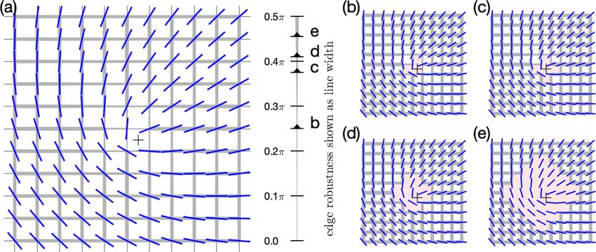
KARL B. HOFFMANN AND IVO F. SBALZARINI                                                      PHYSICAL REVIEW E 103, 012602 (2021)

robustness. We show that the critical vectors, i.e., those for      one singular point x ∈ X , or the topological charge indA (V)
which the smallest change does alter the TD charge, indicate        for general enclosed areas A ⊂ X .1
dislocation directions of defects and locations of likely defect
pair annihilation or generation.                                         B. Identification of topological defects in discrete domains
   The so-defined robustness measure of topological charge
                                                                        We transfer the above definitions for continuous domains
applies to all scales from smallest discretization units to the
                                                                    to vector fields on discrete domains. This requires adapting
whole domain. In addition to enabling defect filtering based
                                                                    the concept of lifting by replacing the continuous closed path
on interpretable robustness thresholds, the proposed measure
                                                                    γ : [0, 1] → X with a finite series of pairwise neighboring
also allows us to quantify the trade-off between the identi-
                                                                    discretization points x0 , x1 , x2 , . . . , xN = x0 ∈ X . Then, lift-
fication robustness of TDs and the spatial precision of their
                                                                    ing V̂ ◦ γ turns into lifting the finite series (V̂(xn ))n=0,...,N . For
localization estimate in discrete domains. This enables the
                                                                    this finite-set domain, continuity as the key defining feature of
quantitative study of defects with large unordered cores, and it
                                                                    liftings is trivial, making any map an admissible lifting.
also enables us to automatically choose the shape and size of
                                                                        To recover uniqueness, one assumes—usually tacitly—the
the neighborhood used for defect identification in a spatially
                                                                    points (xn )n=0,...,N to form a sufficiently fine discretization of
data-adaptive manner to always provide the best trade-off
                                                                    an underlying smooth vector field with a continuous domain
between robustness and localization precision. For this, we
                                                                    (see Appendix B for feasibility). The unit vectors V̂ to be
provide a data-adaptive algorithm for identifying TDs and
                                                                    lifted are from the periodic set RP1 = S∼        1
                                                                                                                       . Analogous to the
their charges in discrete domains, which might serve as a
                                                                    Nyquist-Shannon sampling theorem, correct reconstruction of
starting point for uncertainty quantification of TDs.
                                                                    azimuthal changes from discrete samples is guaranteed if the
                                                                    spatial sampling frequency fs is higher than twice the highest
                                                                    spatial frequency (band limit) Barg of the azimuth. When a
            II. BACKGROUND AND NOTATION
                                                                    continuous representation arg of the azimuth arg (x) obeys
   We start from a definition of TDs in polar and nematic           this condition, the net azimuth change arg(xn ) − arg(xn−1 )
vector fields on continuous domains, from which we then state       between neighboring discretization points stays below π /2
the definition on discrete domains.                                 (below π for polar vectors). Hence, the lifted version h(xn ) −
                                                                    h(xn−1 ) is uniquely determined among all possible azimuth
                                                                    changes by its minimal absolute value ∈ [−π /2, π /2]. De-
         A. Topological defects in continuous domains               fine, for nematic (1) and polar (2) vectors,
    TDs are defined in polar and nematic vector fields of arbi-      modπ : R → [−π /2, π /2) : x → x − π 0.5 + x/π , (1)
trary dimension using homotopy theory [7,31]. Here, we focus
on point defects in two-dimensional fields with continuous flat          mod2π : R → [−π , π ) : x → x − 2π 0.5 + x/(2π )              (2)
domain X ⊆ R2 . On this domain, we consider a polar vector                                          2
field V : X → R2 or a nematic orientation field V : X → R2∼ ,       as the uniquely determined, least absolute value modπ (x) of
where R2∼ is the set of nematic vectors (directors, orienta-        the π -periodic set x + π Z := {x + π z; z ∈ Z} (of x + 2π Z
tions) obtained from R2 by identifying antipodal polar vectors      for polar). For nematic vectors V(xn−1 ), V(xn ) represented
y ∼ −y to one nematic vector [y]∼ := {y, −y} ∈ R2∼ .                by any azimuth θn−1 , θn ∈ R fulfilling V(xk )/V(xk ) =
    The spaces of polar vectors R2 and nematic vectors R2∼ are      V̂(xk ) = [exp (iθk )]∼ , k = n − 1, n, the smallest net az-
isomorphic by halving or doubling, respectively, the azimuth        imuth change then is modπ (θn − θn−1 ) [for polar vectors
(angular coordinate, argument) arg (y) of a complex number          mod2π (θn − θn−1 )].
representation R2 ∼  = C  y = y exp [i arg (y)]. Therefore,         Then, a closed path x0 , x1 , . . . , xN = x0 of winding num-
it suffices to consider nematic vectors y ∈ R2∼ with azimuth        ber one yields the topological charge estimator (TCE) for the
arg (y) ∈ [−π /2, π /2).                                            enclosed charge or index,3
    A topological defect is then defined as an isolated dis-             TCE(x) := TCEx0 ,x1 ,...,xN (x)
continuity x ∈ X of an otherwise continuous vector field V :
                                                                                        1
                                                                                           N
X → R2∼ . TDs are classified by their topological charge or
index, which is half integer (integer for polar vector fields).                   :=          modπ {arg[V(xn )] − arg[V(xn−1 )]},
                                                                                       2π n=1
We calculate the topological charge based on liftings (for de-
tails, see Appendix A). For that, consider the normalized field                                                                         (3)
V̂ : X → RP1 : x → V(x) / V(x). The image space of the
unit nematic vectors RP1 = S∼   1
                                  = {[y]∼ ∈ R2∼ ; y ∈ S 1 }, also
known as the real projective line, has a universal cover             1
                                                                        We assume areas without holes for simplicity, but our robustness
p∼ : R → RP1 ⊆ C∼ : w → [ei2πw ]∼ . Then, for a contin-            results equally apply to the general case.
uous map γ : [0, 1] → X with γ (0) = γ (1) (i.e., a closed            2
                                                                        The least absolute value is ambiguous for x = π /2 mod π , for
path), there exists a “lifted” version of V̂ ◦ γ that is a con-     which we choose modπ (x) = −π /2. This corner case will receive
tinuous map h : [0, 1] → R, such that p∼ ◦ h = V̂ ◦ γ . The         zero robustness anyway; see Eqs. (5) and (6).
lifting h is uniquely determined up to additive multiples of          3
                                                                        Equation (3) applies to areas without holes. An extension to ar-
π , and it counts the number of full rotations of the azimuth       eas with holes is possible by subtracting the charge enclosed by
arg(V) = arg(V̂) along the closed path γ . Hence, h(1) − h(0)       inner paths, to larger winding numbers by splitting paths at self-
defines the Poincaré index indx (V) when γ encloses exactly         intersection points.

                                                              012602-2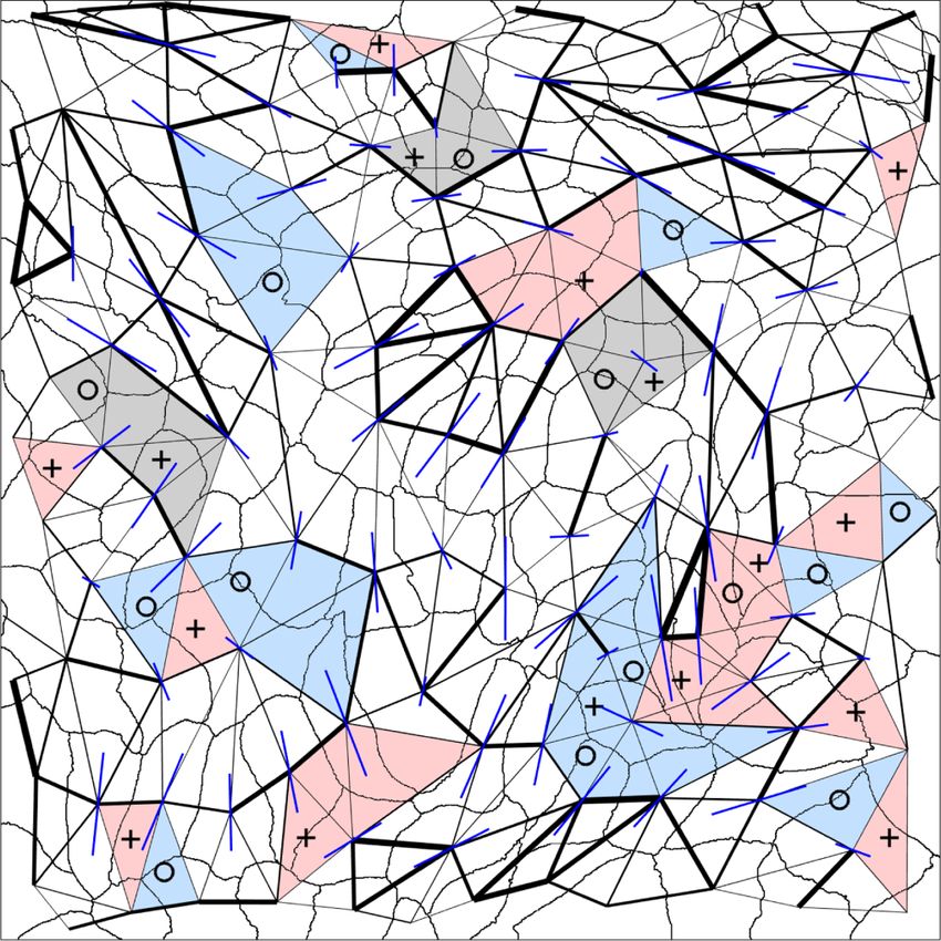
ROBUSTNESS OF TOPOLOGICAL DEFECTS IN DISCRETE …                                                  PHYSICAL REVIEW E 103, 012602 (2021)

    FIG. 1. Estimation of topological charge and its robustness, here shown for nematic vector fields. (a),(b) On a continuous domain, the
normalized vectors along a closed path (green) around (a) a singular point are lifted to (b) a continuously changing azimuth, whose total
change of +π [red half circle in (b)] here indicates a +1/2 defect charge. (c),(d) On a discrete domain, discretized with arbitrary offset
as shown by the thin gray lines in (a), the azimuth changes along finite path steps x0 , . . . , x4 = x0 in (c). The normalized vectors in the
corresponding discrete lifting [Eq. (3)] sum to the same index estimate in (d). (e),(f) Upon continuous change of a vector [compare point x1 in
(c) and (e)], the index estimate discontinuously changes, here to 0 when V(x1 ) crosses the dash-dotted black line perpendicular to V(x0 ).

where any other azimuth representatives θn can replace                    which are defined over connected spaces (intervals) too. Con-
arg [V(xn )]. By construction of Eq. (1), we have modπ (x) =              sequently, the discontinuities of Eq. (3) are not an impairment
x + zπ for some z ∈ Z and, therefore,                                     of that specific estimator. On the contrary, Eq. (3) is optimal,
                                                                          as it only possesses the inevitable discontinuities.
              1
                 N
   TCE =            modπ (θn − θn−1 )                                         Because of the inevitable discontinuities, arbitrarily small
             2π n=1                                                       (critical) aberrations of orientations can cause the topological
                                                                          charge estimate to jump between discrete values. We study the
              1                          1
                 N                           N
                                                    1                     conditions under which topological charge estimates switch
         =          (θn − θn−1 + zn π ) =       zn ∈ Z           (4)      and find exact algebraic expressions for the corresponding
             2π n=1                       2 n=1     2
                                                                          critical azimuth or vector changes. This allows us to define the
yields half-integer values as required for topological charges            robustness of a TD as the smallest azimuth change that alters
[integer values for polar fields, where mod2π replaces modπ               the TCE. This is a natural definition of robustness, as it bounds
in Eqs. (3) and (4)]. This also holds true in numerical imple-            the admissible fluctuations in the vector field. For simplicity,
mentations to the order of machine precision.                             we assume normalized nematic fields to derive the robustness
                                                                          measure and extend to unnormalized fields in Appendix C.
                 III. ROBUSTNESS MEASURE
                                                                                            A. Robustness of a single edge
   We observe that the topological charge estimator in Eq. (3)
does not depend continuously on the input vectors V(xn ) and                 Topological charge estimation by Eq. (4) involves elemen-
their azimuths, as the function modπ (·) has discontinuous                tary net azimuth changes modπ (θn − θn−1 ) corresponding to
jumps of −π at locations π /2 + Z [cf. Eq. (1) and Fig. 1].               path edges (xn−1 , xn ). We thus start by defining edge robust-
Such discontinuous behavior is inevitable for any noncon-                 ness R : R → R0 ,
                                              N
stant map from the connected space (R2∼ ) of orientation                  R(x) := dist(x, π /2+ π Z) = π /2 − |modπ (x)| ∈ [0, π /2],
                                           1
N-tuples to the totally disconnected space 2 Z. Discontinuities                                                                   (5)
are encountered at least between pre-images (TCE)−1 (c1 ),
(TCE)−1 (c2 ) of different topological charges c1 , c2 ∈ 21 Z,               R(x) := dist(x, π + 2π Z) = π − |mod2π (x)| ∈ [0, π ]
c1 = c2 . This equally applies to TCE based on azimuth angles,                                                                             (6)

                                                                  012602-3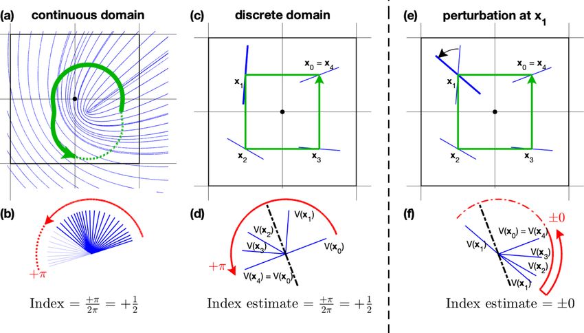
KARL B. HOFFMANN AND IVO F. SBALZARINI                                                              PHYSICAL REVIEW E 103, 012602 (2021)

for nematic and polar vectors, respectively, as the azimuthal                 such applications, here we characterize the behavior of the
distance to the nearest discontinuity of modπ (mod2π for                      robustness measure for fixed shapes of the closed path and
polar). Therefore, the largest symmetric interval of continuity               for data-dependent paths that are implicitly defined through
for modπ (·) around some x0 ∈ R is [x0 − R(x0 ), x0 + R(x0 )],                the considered vector field.
with one-sided extension to interval size π possible. These in-
tervals are where x → modπ (x) − x ∈ π Z is constant. Hence,
the contribution of an edge (xn−1 , xn ) to the TCE remains                                 A. Robustness for fixed path shapes
unaltered if fluctuations θn−1 , θn of azimuths θn−1 , θn obey
                                                                                 When searching for TDs using a fixed path, the size and
            |modπ (θn − θn−1 )| < R(θn − θn−1 ).                     (7)    shape of the path must be decided. The highest localiza-
                                                                              tion accuracy is obtained for paths enclosing one single grid
                                                                              cell. However, for the smallest nonzero topological charge
                 B. Robustness of a complete path
                                                                              ±1/2 to be estimated within a path of length N, there must
    Combining edge robustnesses along a closed path                           be edges of net azimuthal change |θn − θn−1 |  π /N, limit-
x0 , x1 , x2 , . . . , xN = x0 ∈ X , the TCE remains unaltered if             ing the identification robustness to Rx0 ,x1 ,...,xN  π /2 − π /N,
Eq. (7) holds for all n = 1, . . . , N. Each azimuth θn is con-               that is,  π /6 for N = 3 or  π /4 for N = 4. Moreover,
tained in exactly two differences, namely, modπ (θn − θn−1 )                  single-cell paths can yield robustnesses 0 even for perfect
and modπ (θn+1 − θn ), where for simplicity θN+1 := θ1 .                      defects [32].
Hence, the condition in Eq. (7) is certainly fulfilled if azimuth                The identification robustness can be increased by choosing
fluctuations θn are limited4 for all n = 1, . . . , N as                     longer paths that enclose larger areas containing the defect.
                                                                              Indeed, regular points have robustness ∈ [0, π /2), and longer
         |θn | <    1
                     2
                         min{R(θn+1 − θn ), R(θn − θn−1 )}.            (8)    paths around larger areas including a single defect approach
 A common bound for all azimuthal fluctuations along the                      the robustness limit π /2 from below, at the cost of reduced
closed path x0 , x1 , x2 , . . . , xN = x0 ∈ X is given by                    localization accuracy. An optimal trade-off between robust-
                                                                              ness and localization accuracy on regular Cartesian grids was
        |θn | < 21 Rx0 ,x1 ,x2 ,...,xN   for all n = 1, . . . , N,    (9)    found for 2 × 2 or 3 × 3 square paths [32], with 2 × 2 mostly
                                                                              used in the literature (e.g., [1,18]).
where we define path robustness,
            Rx0 ,x1 ,x2 ,...,xN :=  min R(θn − θn −1 ),            (10)
                                   n =1,...,N                                          B. Robustness for data-dependent path shapes
as the minimum over edge robustnesses.                                            Instead of fixing the path beforehand, one can also fix
    Any of the conditions (7), (8), or (9) guarantees an un-                  the desired identification robustness and ask for the finest
altered topological charge estimate by Eq. (4). Each of the                   spatial resolution that achieves this robustness. According
bounds is sharp. They equally apply to singular (topological                  to its definition in Eq. (10), path robustness is defined by
charge = 0) and regular (topological charge = 0) points, as                   the robustness of the critical edge (xnc −1 , xnc ) with nc :=
well as general areas enclosed by paths.                                      argminn=1,...,N R(θn − θn−1 ). To increase robustness, one can
    Then, critical fluctuations θn−1   crit
                                             , θncrit are defined by         replace the critical edge with a new path segment. Let A
modπ (θn − θn−1 ) + (θn − θn−1 ) = ±π /2. This implies
                          crit         crit                                   be the area enclosed by the original path x0 , x1 , . . . , xN =
(θn + θncrit ) − (θn−1 + θn−1crit
                                    ) ∈ π /2 + π Z, which charac-             x0 . Change the path by encompassing a grid cell ai adja-
terizes vectors perpendicular to each other. This means that                  cent to the critical edge. This makes (xnc −1 , xnc ) an interior
the TCE remains unaltered as long as nematic vectors fluc-                    edge of the expanded area A = A + ai and thus irrelevant
tuate without becoming perpendicular (polar vectors: without                  for the robustness of topological charge estimation. Repeat
becoming antipodal) to their neighbors along the path [com-                   this process of “expansion over the critical edge” until the
pare Figs. 1(c) and 1(d) to Figs. 1(e) and 1(f)].                             desired robustness Rthresh is reached; cf. Fig. 2. While this
                                                                              produces irregular path shapes, they are guaranteed to en-
                                                                              close minimally sized areas with robustness  Rthresh . The
          IV. ROBUSTNESS VERSUS PATH SHAPE                                    edges delimiting such minimal-area robust regions form
   The above robustness measure for TDs in discrete domains                   the maximal leaf-free subgraph among all edges with edge
can be used to facilitate or improve the identification of TDs                robustness R  Rthresh .
in data from, e.g., numerical simulations, measurements, or                       Any change in TCE during “expansion over the criti-
images. It can also be used to study the trade-off between the                cal edge” hints at potential locations of additional defects.
robustness with which a TD can be identified and the accuracy                 By construction, robustness changes below Rthresh relo-
with which is can be localized in space [32]. In order to enable              cate nonzero topological charge within the area enclosed
                                                                              by the path, but not beyond. This may include annihi-
                                                                              lation of additional defect pairs that are only separable
                                                                              with robustness
ROBUSTNESS OF TOPOLOGICAL DEFECTS IN DISCRETE … PHYSICAL REVIEW E 103, 012602 (2021)
FIG. 2. Data-dependent iterative path adaptation. (a) Example defect from Fig. 1 discretized on a regular Cartesian grid. Edge robustness
is shown by line thickness scaling as robustness to the fourth power; “+” marks the grid cell containing defect charge +1/2. (b)–(e) Requiring
robustness above thresholds of Rthresh /(0.5π ) = (b) 0.50, (c) 0.75, (d) 0.82, and (e) 0.91 (arrowheads on the robustness scale) adaptively
increases the area (shaded red) enclosed by the path. All surrounding grid cells have index estimate 0 with high robustness, already at the finest
resolution.
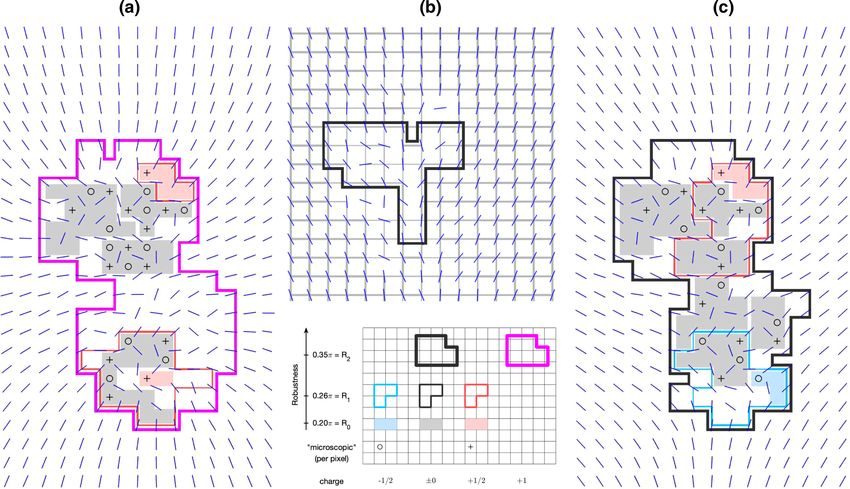
FIG. 3. Robust identification of TDs. (a) Detection of higher-order TDs (here, +1) is possible. Comparing robustness levels R1 and R2 ,
splitting into or merging from elementary charges (here, two times +1/2) can be detected. (b) Large unordered region with interior edges
of low robustness indicates potential pair generation prior to the formation of “microscopic” charges. For visualization, the line width of the
edges scales as the fourth power of robustness as in Fig. 2; edges below robustness R1 are omitted. (c) Adjustment of detection area to the data
at unordered cores (R0 vs R1 versus microscopic charges). Anisotropic growth of detection areas at higher robustness indicates the direction
of defect motion. Zero total charge at the highest robustness R2 indicates potential pair annihilation. The legend is common to all panels. For
clarity, shading of zero-charge regions without microscopic defect(s) has been omitted in all panels.
012602-5KARL B. HOFFMANN AND IVO F. SBALZARINI PHYSICAL REVIEW E 103, 012602 (2021)
order defects can be identified5 without postprocessing; see to irregularly spaced data and arbitrary discretization grids,
Fig. 3(a). and to any path shape from enclosing individual grid cells to
Tuning Rthresh trades off robustness versus localization ac- domain-scale areas. Using the proposed robustness measure,
curacy. For 0 Rthresh,1 < Rthresh,2 , the path determined for we have derived upper bounds for the maximum robustness
Rthresh,1 is contained within the path for Rthresh,2 . The per- achievable using paths of fixed length, and we have argued
cell robustness increase can be used to hint at locations of for a trade-off between estimation robustness and localiza-
likely or imminent defect pair annihilation or generation. tion accuracy. Further, we have proposed data-driven iterative
Defect pair generation is likely inside zero-charge areas that adaptation of paths (“expansion over the critical edge”) until a
contain multiple edges of low robustness; see Fig. 3(b). De- given robustness threshold is reached, and we have discussed
fect pair annihilation is indicated by opposite topological how this may hint at defect dislocation, pair annihilation or
charges separated at low robustness threshold Rthresh,1 0, generation, and unordered defect cores.
but merged at higher Rthresh,2 > Rthresh,1 ; see Fig. 3(c). This The idea of data-dependent paths is not new. For example,
confirms classification as pair annihilation for cases reported Ref. [24] constructed adaptive square paths with maximal
in the literature [22], where defects were identified from or- distance to TDs in order to indirectly minimize vector field
der parameters using paths of zero net charge. Finally, likely distortions along the paths. However, the concept of edge ro-
directions of defect dislocation are indicated by anisotropic bustness as defined here generalizes these ideas to nonsquare
growth of the detection area for increasing robustness thresh- path shapes with optimal localization accuracy for a given
olds; see Fig. 3(c). robustness threshold.
Our geometric robustness measure also enables TD filter-
V. EXTENSIONS ing in noisy or uncertain vector fields without presmoothing of
the vector field and without predefined path shapes [1,14,17],
The examples so far considered normalized vector fields defect core length scales [18], or order parameter thresh-
V : X → RP1 (for polar V : X → S 1 ), where robustness is olds [14,22]. This reduces the risk of “masking” (e.g., by
purely azimuthal robustness. Information encoded in the vec- smoothing) defect pairs and of detecting spurious (e.g., noise-
tor magnitude, such as speed in flow fields or coherence in induced) defects. In spatiotemporal vector data, our measure
nematic orientation fields, can be accounted for by defin- can be used to predict defect dynamics (appearance, annihi-
ing magnitude-aware robustness of TDs for unnormalized lation, dislocation) when temporal changes of vectors exceed
fields V : X → R2∼ (for polar V : X → R2 ), as shown in the robustness threshold. This is especially valuable for study-
Appendix C. ing active nematic and active polar materials, which show rich
We also so far only considered regular Cartesian grids. behavior of TDs [9–11,13,14,33].
However, the present robustness measure readily extends to Combining the proposed robustness measure with a noise
other grid types, including triangulations of unstructured data model for the vector data could lead to topological uncer-
(see Appendix D). The theory only requires closed paths. tainty quantification, e.g., in nematic liquid crystals, solid
Data-dependent path adaptation extends to arbitrary grids by state physics, material science, fluid mechanics, and biolog-
iteratively adding non-Cartesian grid cells over the critical ical physics. Such noise models for the vector field may, e.g.,
edge. be available for numerical simulations from numerical error
estimators, or for digital images from camera noise models
VI. CONCLUSION AND DISCUSSION and image-processing uncertainty. Then, the present robust-
ness measure defines a noise model or uncertainty on the level
We have proposed a robustness measure for topological of TDs.
defects (TDs) and their charges in discrete domains. Topolog- We restricted our considerations to point defects on flat
ical charge is necessarily a discontinuous map for polar and two-dimensional domains. A generalization to point de-
nematic vector fields on discretized domains, as they typically fects on n-dimensional domains, to curved manifolds, or
occur in computer simulations, measurement data, and digi- to k-dimensional (0 < k < n) defects seems difficult (see
tal images. Our continuous robustness measure complements Appendix E) and remains an open problem. Lastly, our ap-
the discrete values of topological charge (0, ±1/2, ±1, . . .), proach requires the robustness threshold to be set. We find
either in azimuthal or vector space. It quantifies the largest ad- that a quantile from the distribution of individual edge robust-
missible vector variation everywhere in the neighborhood of nesses works well in practice.
a TD that does not alter the estimated topological charge, also Notwithstanding these limitations and open issues, the
for regular, defect-free areas. This provides an interpretable present results provide a starting point for robust and noise-
notion of robustness that directly links to the underlying aware defect analysis in discretized data, and they are easily
data. integrated into the standard process of defect identification.
The proposed robustness measure can efficiently be com-
puted, as it is based on the same path edges and vectors as
topological charge estimation itself. The measure also ap- APPENDIX A: DEFINITION OF TOPOLOGICAL
plies to higher-order defects without additional processing, CHARGE BY LIFTING
We define the index or topological charge based on lift-
ings. There are equivalent definitions in terms of homotopy
5
Because of higher net azimuth change, they require longer paths groups or by the Brouwer degree in homology groups [31].
anyway and cannot be found on single grid cells. The latter indirectly uses liftings as well, but we prefer to
012602-6ROBUSTNESS OF TOPOLOGICAL DEFECTS IN DISCRETE … PHYSICAL REVIEW E 103, 012602 (2021)
make the lifting explicit for a clearer transition to the discrete APPENDIX B: FEASIBILITY OF A SUFFICIENTLY FINE
case. DISCRETIZATION
Consider the space of unit nematic vectors RP1 = S∼ 1
=
There is always a resolution above which discretization of
{[x]∼ ∈ R∼ ; x ∈ S }, also known as the real projective line,
2 1
a vector field yields a discretized path that fulfills the Nyquist-
and its universal cover,
Shannon sampling theorem. To see this, consider a closed path
p∼ : R → RP1 ⊆ C∼ : w → [ei2πw ]∼ . (A1) γ , not touching any singular points, in a vector field on a
continuous domain. Since the closed path γ : [0, 1] → X is
Then, for any nematic vector field V : X → R2∼ and any continuous, the vector field is continuous by assumption, and
closed path γ not touching zeros of V, that is, γ : [0, 1] → X the map arg : R2∼ → RP1 is away from singular points, the
continuous with γ (0) = γ (1), the universal cover p∼ allows concatenation arg ◦V ◦ γ : [0, 1] → RP1 is continuous on a
lifting the normalized vector field V̂ : X → RP1 : x → V(x)
V(x) compact domain, and hence Lipschitz continuous with some
along γ , i.e., it guarantees the existence of a continuous Lipschitz constant L. Therefore, a discretization of the path
map h : [0, 1] → R into the covering space R representative with spacingKARL B. HOFFMANN AND IVO F. SBALZARINI PHYSICAL REVIEW E 103, 012602 (2021)
the topological charge estimator as introduced in Eq. (3). The
path robustness remains as defined in Eq. (10).
APPENDIX E: HIGHER DIMENSIONS AND CURVED
MANIFOLDS
Generalizing the present robustness measure to higher di-
mensions seems difficult. We explain where this difficulty
comes from, without being able to provide solutions. A gener-
alization to point defects on n-dimensional domains would re-
quire considering discretized forms of the maps S n−1 → S n−1
and S n−1 → S∼ n−1
that define the topological charge of point
defects in the homotopy group πn−1 (S n−1 ) [7]. This group is
isomorphic to Z, as is π1 (S 1 ) in the two-dimensional case. The
difficulty is to determine the homotopy class ∈ πn−1 (S n−1 )
that vectors on a finite discretized neighborhood represent.
When this is done locally, one must additionally assure that
the local representatives fit together globally. This joining is
straightforward in two-dimensional fields, where the edges
only connect in points. However, in n-dimensional fields, it
is unclear how to join the (n − 1)-dimensional hypersurface
pieces of S n−1 along a complete submanifold of dimension up
FIG. 4. Robust identification of TDs in non-Cartesian data. We
to n − 2. Extending the data-dependent choice of the region
show an example of an irregular planar graph (thin, curved solid for topological charge estimation also requires extra care in
lines) extracted from an image of biological cells. Connecting the cell higher dimensions, as the boundary—in 2D formed by the
centers converts this graph to a planar triangulation (straight solid edges—needs to maintain the topology of an S n−1 sphere.
lines; line width scales as fourth power of edge robustness). Such These difficulties amplify for k-dimensional (1 k <
conversion is always possible for planar graphs in two dimensions n) defects in discretized vector fields over n-dimensional
(2D). Blue sticks visualize the elongation and orientation of the domains. Such defects are extended objects that can (self-
cells in the original graph, computed from their tensor of inertia. )intersect [34], and already the identification of line (k = 1)
“Microscopic” topological charges are visualized by symbols (+ for defects in three dimensions requires an iterative process [35].
+1/2, o for −1/2). Areas found by “expansion over critical edge” In this special case, planar cuts through a line defect yield
for robustness threshold 0.25π are shown shaded (blue: total charge point defects in two dimensions, and our presented robustness
+1/2; red: total charge −1/2; gray: total charge 0 if they contain could be applied within each plane. However, the paths within
microscopic defects). each plane have to join topologically correctly to a cylinder
or torus enclosing the whole line defect, which defines similar
all results for azimuthal robustness transfer to the magnitude- difficulties as the construction of an enclosing hypersurface
aware case by limiting each vectorial change along a closed for point defects in dimensions 3.
path xn , n = 1, . . . , N, as Another possible extension is to two-dimensional curved
manifolds, with the azimuthal difference between vectors in
V(xn ) < 1
2
min{Rmagn [V(xn ), V(xn−1 )], tangent spaces of different discretization points defined by
parallel transport. Note that parallel transport itself is path
Rmagn [V(xn ), V(xn+1 )]}. (C2)
dependent, such that the angle change accumulated by parallel
For other measures of magnitude, e.g., the infinity norm, transporting along a closed path is equal to the integral over
magnitude-aware robustness can be constructed similarly. the enclosed curvature. Hence, for TDs located in regions of
curvature of equal sign, the parallel transport already covers
parts of the net azimuthal change required for defect identi-
APPENDIX D: NON-CARTESIAN DISCRETIZATIONS
fication. For example, ±1/2 defects on curved manifolds can
We outline how the present ideas, in particular the ro- therefore be identified from a path of length N with robustness
bustness measure and the data-adaptive paths, extend to above the threshold π /N valid in flat domains (see Sec. IV A).
non-Cartesian discretizations. Since any spatial distribution of This is compatible with the experimental and simulation re-
discretization points in 2D can always be represented as a tri- sults suggesting that TDs prefer to be in regions of maximal
angulation, it is sufficient to show how to extend to triangular curvature of the same sign as the defect charge [13,14,36]. A
meshes, as shown in the example in Fig. 4. The concepts and high defect robustness, according to the definition provided
definitions introduced here only require a planar graph with here, then relates to energetically favorable minimization of
discretization points as vertices. We made no assumptions field distortions between neighboring discretization points,
about the geometry of the graph. Each of the edges between observed only along the associated loop path rather than inte-
two discretization points can be assigned an edge robustness grated over the whole field. Therefore, the present robustness
as defined in Sec. III A. For any area bounded by a single loop measure makes explicit a coupling between the topology and
in the planar graph, the topological charge is then given by geometry in curved domains.
012602-8ROBUSTNESS OF TOPOLOGICAL DEFECTS IN DISCRETE … PHYSICAL REVIEW E 103, 012602 (2021)
[1] A. M. Bazen and S. H. Gerez, Systematic methods for the [21] J. Colen, M. Han, R. Zhang, S. A. Redford, L. M. Lemma, L.
computation of the directional fields and singular points of Morgan, P. V. Ruijgrok, R. Adkins, Z. Bryant, Z. Dogic, M. L.
fingerprints, IEEE Trans. Pattern Analys. Mach. Intell. 24, 905 Gardel, J. J. De Pable, and V. Vitelli, Machine learning active-
(2002). nematic hydrodynamics, arXiv:2006.13203.
[2] W. Bian, D. Xu, Q. Li, Y. Cheng, B. Jie, and X. Ding, A survey [22] H. Qian and G. F. Mazenko, Vortex dynamics in a coars-
of the methods on fingerprint orientation field estimation, IEEE ening two-dimensional XY model, Phys. Rev. E 68, 021109
Access 7, 32644 (2019). (2003).
[3] P. Avelino, T. Barreiro, C. S. Carvalho, A. Da Silva, F. S. Lobo, [23] L. Angheluta, P. Jeraldo, and N. Goldenfeld, Anisotropic veloc-
P. Martin-Moruno, J. P. Mimoso, N. J. Nunes, D. Rubiera- ity statistics of topological defects under shear flow, Phys. Rev.
Garcia, D. Saez-Gomez et al., Unveiling the dynamics of the E 85, 011153 (2012).
universe, Symmetry 8, 70 (2016). [24] A. U. Oza and J. Dunkel, Antipolar ordering of topological
[4] J. C. Teo and T. L. Hughes, Topological defects in symmetry- defects in active liquid crystals, New J. Phys. 18, 093006
protected topological phases, Annu. Rev. Condens. Matter (2016).
Phys. 8, 211 (2017). [25] D. Wenzel, M. Nestler, S. Reuther, M. Simon, and A. Voigt,
[5] P.-G. De Gennes and J. Prost, The Physics of Liquid Crystals, Defects in active nematics: Algorithms for identification and
2nd ed., Vol. 83 (Oxford University Press, Oxford, 1995). tracking, arXiv:2002.02748.
[6] M. J. Bowick and L. Giomi, Two-dimensional matter: Order, [26] B. Jähne, Spatio-Temporal Image Processing: Theory and Sci-
curvature and defects, Adv. Phys. 58, 449 (2009). entific Applications, Lecture Notes in Computer Science, Vol.
[7] N. D. Mermin, The topological theory of defects in ordered 751 (Springer, Heidelberg, Germany, 1993).
media, Rev. Mod. Phys. 51, 591 (1979). [27] Z. Püspöki, M. Storath, D. Sage, and M. Unser, Transforms
[8] S. Shankar, A. Souslov, M. J. Bowick, M. C. Marchetti, and V. and operators for directional bioimage analysis: A survey, in
Vitelli, Topological active matter, arXiv:2010.00364. Focus on Bio-Image Informatics, edited by W. H. De Vos, S.
[9] L. Giomi, M. J. Bowick, P. Mishra, R. Sknepnek, and M. Munck, and J.-P. Timmermans (Springer, Cham, Switzerland,
Cristina Marchetti, Defect dynamics in active nematics, Philos. 2016), pp. 69–93.
Trans. R. Soc. A 372, 20130365 (2014). [28] M. Merkel, R. Etournay, M. Popović, G. Salbreux, S. Eaton,
[10] C. Peng, T. Turiv, Y. Guo, Q.-H. Wei, and O. D. Lavrentovich, and F. Jülicher, Triangles bridge the scales: Quantifying cellular
Command of active matter by topological defects and patterns, contributions to tissue deformation, Phys. Rev. E 95, 032401
Science 354, 882 (2016). (2017).
[11] A. Doostmohammadi, J. Ignés-Mullol, J. M. Yeomans, and F. [29] T. B. Saw, A. Doostmohammadi, V. Nier, L. Kocgozlu, S.
Sagués, Active nematics, Nat. Commun. 9, 3246 (2018). Thampi, Y. Toyama, P. Marcq, C. T. Lim, J. M. Yeomans, and
[12] S. Praetorius, A. Voigt, R. Wittkowski, and H. Löwen, Active B. Ladoux, Topological defects in epithelia govern cell death
crystals on a sphere, Phys. Rev. E 97, 052615 (2018). and extrusion, Nature (London) 544, 212 (2017).
[13] F. C. Keber, E. Loiseau, T. Sanchez, S. J. DeCamp, L. Giomi, [30] M. A. Bates, Nematic ordering and defects on the surface of a
M. J. Bowick, M. C. Marchetti, Z. Dogic, and A. R. Bausch, sphere: A Monte Carlo simulation study, J. Chem. Phys. 128,
Topology and dynamics of active nematic vesicles, Science 345, 104707 (2008).
1135 (2014). [31] G. E. Bredon, Topology and Geometry, 2nd ed., edited by J. H.
[14] P. W. Ellis, D. J. Pearce, Y.-W. Chang, G. Goldsztein, L. Giomi, Ewing, F. W. Gehring, and P. R. Halmos, Graduate Texts in
and A. Fernandez-Nieves, Curvature-induced defect unbinding Mathematics, Vol. 139 (Springer-Verlag, New York, 1995).
and dynamics in active nematic toroids, Nat. Phys. 14, 85 [32] K. B. Hoffmann and I. F. Sbalzarini, A robustness measure
(2018). for singular point and index estimation in discretized orienta-
[15] G. Duclos, C. Erlenkämper, J.-F. Joanny, and P. Silberzan, tion and vector fields, Proc. Appl. Math. Mech. 20, 16938700
Topological defects in confined populations of spindle-shaped (2020).
cells, Nat. Phys. 13, 58 (2017). [33] R. Ramaswamy, G. Bourantas, F. Jülicher, and I. F. Sbalzarini,
[16] K. Kawaguchi, R. Kageyama, and M. Sano, Topological defects A hybrid particle-mesh method for incompressible active polar
control collective dynamics in neural progenitor cell cultures, viscous gels, J. Comput. Phys. 291, 334 (2015).
Nature (London) 545, 327 (2017). [34] S. Čopar, J. Aplinc, Ž. Kos, S. Žumer, and M. Ravnik, Topology
[17] J.-M. Guo, Y.-F. Liu, J.-Y. Chang, and J.-D. Lee, Fingerprint of Three-Dimensional Active Nematic Turbulence Confined to
classification based on decision tree from singular points and Droplets, Phys. Rev. X 9, 031051 (2019).
orientation field, Expert Syst. Applic. 41, 752 (2014). [35] G. Duclos, R. Adkins, D. Banerjee, M. S. Peterson, M.
[18] S. J. DeCamp, G. S. Redner, A. Baskaran, M. F. Hagan, and Z. Varghese, I. Kolvin, A. Baskaran, R. A. Pelcovits, T. R. Powers,
Dogic, Orientational order of motile defects in active nematics, A. Baskaran, F. Toschi, M. F. Hagan, S. J. Streichan, V. Vitelli,
Nat. Mater. 14, 1110 (2015). D. A. Beller, and Z. Dogic, Topological structure and dynam-
[19] M. L. Blow, S. P. Thampi, and J. M. Yeomans, Biphasic, Ly- ics of three-dimensional active nematics, Science 367, 1120
otropic, Active Nematics, Phys. Rev. Lett. 113, 248303 (2014). (2020).
[20] A. Doostmohammadi, S. P. Thampi, and J. M. Yeomans, [36] F. Alaimo, C. Köhler, and A. Voigt, Curvature controlled defect
Defect-Mediated Morphologies in Growing Cell Colonies, dynamics in topological active nematics, Sci. Rep. 7, 5211
Phys. Rev. Lett. 117, 048102 (2016). (2017).
012602-9You can also read