Role Of the Sun and the Middle atmosphere/thermosphere/ionosphere In Climate (ROSMIC): a retrospective and prospective view - Progress in Earth ...
←
→
Page content transcription
If your browser does not render page correctly, please read the page content below
Ward et al. Progress in Earth and Planetary Science             (2021) 8:47
https://doi.org/10.1186/s40645-021-00433-8
                                                                                                                               Progress in Earth and
                                                                                                                                  Planetary Science

 REVIEW                                                                                                                                          Open Access

Role Of the Sun and the Middle
atmosphere/thermosphere/ionosphere In
Climate (ROSMIC): a retrospective and
prospective view
William Ward1*† , Annika Seppälä2† , Erdal Yiğit3 , Takuji Nakamura4 , Claudia Stolle5 , Jan
Laštovička6 , Thomas N. Woods7 , Yoshihiro Tomikawa4 , Franz-Josef Lübken8 , Stanley C. Solomon9 , Daniel R.
Marsh9,10 , Bernd Funke11 and Duggirala Pallamraju12

  Abstract
  While knowledge of the energy inputs from the Sun (as it is the primary energy source) is important for understanding
  the solar-terrestrial system, of equal importance is the manner in which the terrestrial part of the system organizes
  itself in a quasi-equilibrium state to accommodate and re-emit this energy. The ROSMIC project (2014–2018 inclusive)
  was the component of SCOSTEP’s Variability of the Sun and Its Terrestrial Impact (VarSITI) program which supported
  research into the terrestrial component of this system. The four themes supported under ROSMIC are solar influence
  on climate, coupling by dynamics, trends in the mesosphere lower thermosphere, and trends and solar influence in
  the thermosphere. Over the course of the VarSITI program, scientific advances were made in all four themes. This
  included improvements in understanding (1) the transport of photochemically produced species from the
  thermosphere into the lower atmosphere; (2) the manner in which waves produced in the lower atmosphere
  propagate upward and influence the winds, dynamical variability, and transport of constituents in the mesosphere,
  ionosphere, and thermosphere; (3) the character of the long-term trends in the mesosphere and lower thermosphere;
  and (4) the trends and structural changes taking place in the thermosphere. This paper reviews the progress made in
  these four areas over the past 5 years and summarizes the anticipated research directions in these areas in the future.
  It also provides a physical context of the elements which maintain the structure of the terrestrial component of this
  system. The effects that changes to the atmosphere (such as those currently occurring as a result of anthropogenic
  influences) as well as plausible variations in solar activity may have on the solar terrestrial system need to be
  understood to support and guide future human activities on Earth.
  Keywords: Climate, Atmosphere, Middle atmosphere, Thermosphere, Ionosphere, Solar irradiance, Energetic
  particles, Atmospheric coupling, Trends

*Correspondence: wward@unb.ca
† William Ward and Annika Seppälä contributed equally to this work.
1
  Department of Physics, University of New Brunswick, POBox 4400,
Fredericton, Canada
Full list of author information is available at the end of the article

                                          © The Author(s). 2021 Open Access This article is licensed under a Creative Commons Attribution 4.0 International License, which
                                          permits use, sharing, adaptation, distribution and reproduction in any medium or format, as long as you give appropriate credit
                                          to the original author(s) and the source, provide a link to the Creative Commons licence, and indicate if changes were made. The
                                          images or other third party material in this article are included in the article’s Creative Commons licence, unless indicated
                                          otherwise in a credit line to the material. If material is not included in the article’s Creative Commons licence and your intended
                                          use is not permitted by statutory regulation or exceeds the permitted use, you will need to obtain permission directly from the
                                          copyright holder. To view a copy of this licence, visit http://creativecommons.org/licenses/by/4.0/.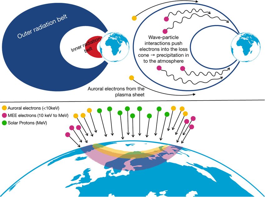
Ward et al. Progress in Earth and Planetary Science   (2021) 8:47                                                      Page 2 of 38

1 Introduction                                                      plays an active role in determining the character of the
The primary goal of solar terrestrial physics is to under-          system and its response to variations in solar input. On
stand the physical foundations of the structures and vari-          average, the terrestrial component of the system is in equi-
ability associated with the coupled Sun-Earth system. The           librium with respect to solar inputs, i.e., the incoming and
challenges are significant, since the important physics of          outgoing energy fluxes are equal. However, the physical
the various components of this system (Sun, Solar wind,             properties of the terrestrial system and the non-local and
magnetosphere, ionosphere, and atmosphere) differ and               non-linear processes that are involved determine the form
dominate in different spatial regions. Furthermore, the             that this equilibrium takes and its response to variations
important time scales of the atmospheric responses to               in solar input.
the forcings become longer closer to the surface of the                Two scientific issues stimulated work to develop insight
Earth. Significant progress has been made in understand-            into the terrestrial response. The first was that while sig-
ing the physics within each region. However, to facilitate          nificant sensitivity to solar variability in the stratosphere
progress, the boundary conditions linking the compo-                and troposphere is observed, the mechanisms causing
nents have tended to be simplified. As a result, interac-           these dependencies are difficult to determine (Gray et al.
tions between the different regions have not been realistic,        2010). The second was the recognition that, in addition
and a full Sun to Earth system description has not been             to radiation and energetic particles, much of the com-
developed.                                                          munication between layers of the atmosphere is due to
  Recently, progress on establishing a full physically self-        waves (most of which are excited in the troposphere)
consistent understanding of the solar-terrestrial system            and that these waves propagate to significant heights
has been made. This is due to the development of new                and cause ionospheric and thermospheric variability
observational techniques, advances in the sophistication            (Oberheide et al. 2015).
and computing power of models, and the generation of                   Over the course of the ROSMIC project, research into
tools allowing processes from the Sun to the Earth to               these issues has continued, and although they have not
be visualized and analyzed. This evolution is reflected             been settled, our understanding has advanced. The incon-
in the nature of recent Scientific Committee on Solar-              sistency between different observations and methods to
Terrestrial Physics (SCOSTEP) programs where investiga-             determine the solar spectral irradiance variations is being
tion of the coupling between regions has been encouraged            resolved (Woods et al. 2015, 2018, Yeo et al. 2017).
(see Shiokawa and Georgieva (2021)).                                Together with total solar irradiance, solar spectral irradi-
  The recently completed VarSITI program (Variability               ance is now being included along with energetic particle
of the Sun and Its Terrestrial Impact, 2014–2019) sup-              forcing as input to model runs for the Coupled Model
ported four projects: SEE (Solar Evolution and Extrema),            Intercomparison Project Phase 6 (CMIP6) of the World
MiniMax24/ISEST (International Study of Earth-affecting             Climate Research Program (Matthes et al. 2017). Inves-
Solar Transients), SPeCIMEN (Specification and Predic-              tigations to identify the subtle processes leading to the
tion of the Coupled Inner-Magnetospheric Environment),              solar influence of the lower atmosphere are progressing,
and ROSMIC (Role Of the Sun and the Middle atmo-                    and new challenges have been identified (Gordon 2020;
sphere/thermosphere/ ionosphere In Climate). Interac-               Dhomse et al. 2016; Thiéblemont et al. 2015; Chiodo et
tions between the various projects were encouraged. In              al. 2019). New complexities in the upward coupling from
PRESTO (PREdictability of variable Solar-Terrestrial cOu-           the troposphere and stratosphere to the mesosphere, ther-
pling), the 2020–2024 SCOSTEP science program, the                  mosphere, and ionosphere associated with waves are now
system aspects of solar-terrestrial relations is further            being addressed. These include recognition of the impor-
emphasized by defining projects in terms of their tempo-            tance of secondary gravity wave generation to wave pen-
ral and spatial relationships through the full system.              etration into the thermosphere (Becker and Vadas 2018)
  The ROSMIC project was devoted to understanding the               and pole-to-pole coupling of dynamical signatures (Karls-
impact of the Sun on the Earth’s middle atmosphere/lower            son and Becker 2016; Smith et al. 2020) and that the pres-
thermosphere/ionosphere (MALTI) and its tropospheric                ence of wave signatures in the thermosphere and iono-
climate. It sought to estimate the importance of this natu-         sphere need not be due to direct propagation (Miyoshi
ral forcing over time scales from minutes to centuries, in          and Yamazaki 2020). Sudden stratospheric warmings and
a world where anthropogenic forcing is driving large-scale          their global influences are being extensively studied (But-
changes across all atmospheric regions. It was a continua-          ler et al. 2015; Pedatella et al. 2018a). They are the largest
tion of the science initiated during the CAWSES (Climate            perturbations to the middle atmosphere on record and
And Weather of the Sun-Earth System) programs under                 provide insights into the mechanisms of the coupling
which many of the intricacies and subtleties of the solar-          between atmospheric layers.
terrestrial system started to be recognized. The essential             The need for coordinated ground observations and
insight was that the terrestrial component of the system            campaigns and associated modeling started to be
Ward et al. Progress in Earth and Planetary Science   (2021) 8:47                                                    Page 3 of 38

addressed during ROSMIC. Examples include the Inter-                from below. The fourth section consists of a summary
hemispheric Coupling Study by Observations and Model-               of progress in observing and understanding long-term
ing (ICSOM) project, the Antarctic Gravity Wave Instru-             trends in the mesosphere and thermosphere (this includes
ment Network (ANGWIN) (Moffat-Griffin et al. 2019),                 progress associated with themes 3 and 4). The paper con-
and The Deep Propagating Gravity Wave Experiment                    cludes with a summary and thoughts on future progress in
(DeepWave) (Fritts et al. 2016). Modeling advanced sig-             this area.
nificantly with whole atmosphere models increasing in
sophistication and including the ionosphere (Liu et al.             2 Overview: general physical principles of the
2018; Miyoshi et al. 2018; Solomon et al. 2019), and data             energetics and organization of the
assimilation efforts start to include mesospheric observa-            atmosphere/ionosphere
tions (Eckermann et al. 2018).                                      Identifying the mechanisms which underlie the mean
  The scientific questions which guided ROSMIC activi-              global atmospheric and ionospheric structures and their
ties were as follows:                                               variability is especially important at this time. First, we
  • What is the impact of solar forcing on the entire               do not fully understand the processes which couple the
                                                                    various regions of the atmosphere and ionosphere. Sec-
    atmosphere? What is the relative importance of
                                                                    ond, uncertainties remain in establishing the extent to
    variability in solar irradiance versus energetic
                                                                    which these structures and their variability might change
    particles?
  • How are the solar signals transferred between the               in response to changes to solar inputs and/or to anthro-
                                                                    pogenically driven changes to atmospheric composition
    thermosphere and the troposphere?
  • How does coupling within the terrestrial atmosphere             (especially those involved in radiative effects in the atmo-
                                                                    sphere). Either of these directly changes the thermal struc-
    function (e.g., what are the roles of gravity waves and
                                                                    ture and circulation of the atmosphere and initiates a
    turbulence?).
  • What is the impact of anthropogenic activities on the           cascade of secondary effects associated with atmospheric
                                                                    waves and their filtering and the transport of radiatively
    MALTI?
  • Why does the MALTI show varying forms of                        active constituents. As noted in more detail below, many
                                                                    of these effects are non-linear and non-local and point to
    long-term variations?
  • What are the characteristics of reconstructions and             the complex and active character of the terrestrial part of
                                                                    the solar-terrestrial system.
    predictions of TSI and SSI?
  • What are the implications of trends in the                        The zeroth-order energy balance between solar radia-
                                                                    tion incident on the Earth and outgoing radiation from
    ionosphere/thermosphere for technical systems such
                                                                    the Earth is well known and covered in most atmo-
    as satellites?
                                                                    spheric texts. More complex considerations of the nature
During VarSITI, ROSMIC supported the activity in the                of this balance for the lower atmosphere can be found
community through existing activities (i.e., Workshop on            in review papers (Trenberth et al. 2009; von Schuck-
Coupling in the Atmosphere-Ionosphere System, ANtar-                mann et al. 2016) where the effects of wind and current
tic Gravity Wave Instruments Network (ANGWIN), High                 systems and eddies are also quantified. Thermodynamic
Energy Particle Precipitation in the Atmosphere/SOLAR               considerations, involving the analysis of the total energy
Influences for SPARC (Stratospheric Processes and                   of the atmosphere (the sum of the internal and poten-
their Role in Climate) (HEPPA-SOLARIS) Workshop,                    tial) relative to the energy of an isothermal reference
13th International Workshop on Layered Phenomena                    atmosphere, provide some constraints on the partitioning
in the Mesopause Region (LPMR), and 9th IAGA -                      of the energy. Recent analysis along these lines (Ban-
ICMA/IAMAS - ROSMIC/VarSITI/SCOSTEP workshop                        non 2013) shows that the percentage of the total energy
on Long-Term Changes and Trends in the Atmosphere)                  of the atmosphere (2.5 Giga Joules) available for atmo-
as well as through the organization of sessions at interna-         spheric motion (termed available potential energy) is a
tional meeting such at COSPAR, IUGG, and the VarSITI                small percentage (< 1%) of the total energy although these
symposia.                                                           motions are responsible for much of the meridional trans-
  This paper is organized as follows. The topic is intro-           port of energy toward the poles. This implies that much
duced in an overview section which summarizes the                   of the absorbed solar energy is devoted to maintaining
physical context underlying the atmosphere/ionosphere               the internal and potential energy of the atmosphere with
components of the Sun/Earth system. This is followed by             a small amount being available for motion. In his analy-
two sections which address the progress in the two most             sis, Bannon (2013) suggests that the rate of conversion of
significant pathways for modulation and propagation of              available energy to kinetic energy is ∼ 5-7 W m−2 . While
atmospheric/ionospheric responses to solar variability to           this is small relative to the solar constant, 1361 W/m2 , it
solar variability namely coupling from above and coupling           plays an essential role in the terrestrial response to solar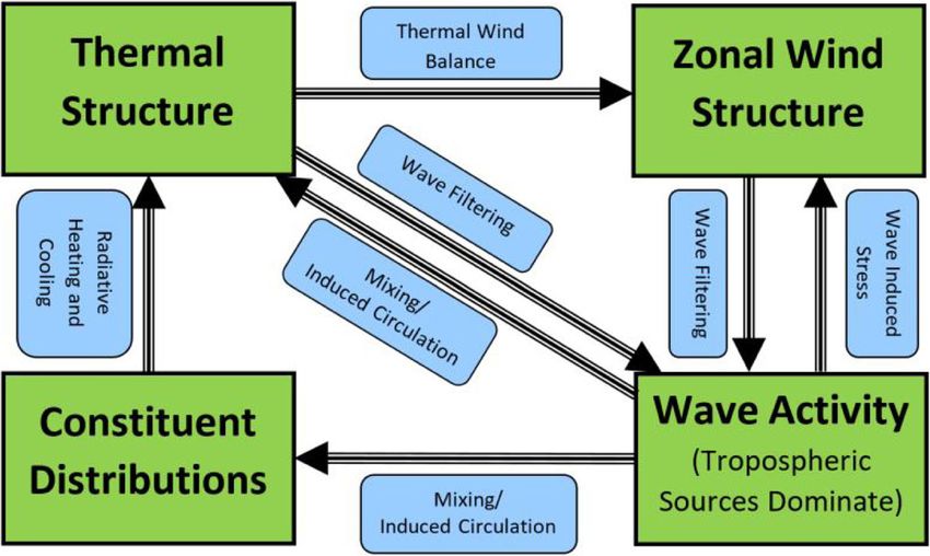
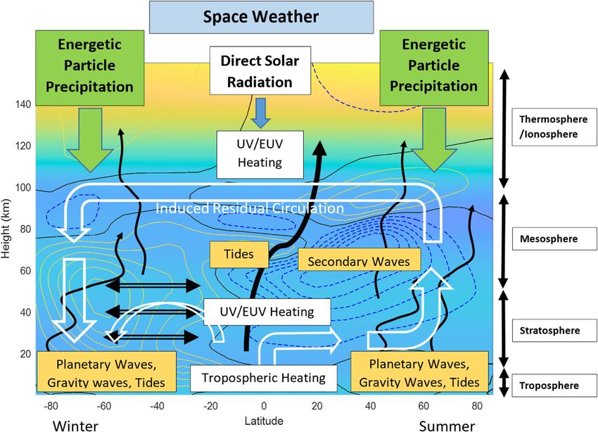
Ward et al. Progress in Earth and Planetary Science     (2021) 8:47                                                                   Page 4 of 38

radiation, as it is associated with the poleward transport                    Figures 2 and 3 are overview figures which provide a
of energy and the global distribution of radiatively active                context for the processes and phenomena discussed later
constituents. An analysis along these lines, which identi-                 in this paper. Figure 2 is a schematic of the drivers of
fies the vertical variation of the partitioning of the incident            the coupling processes noted above. The solstice zonal
energy, appears not to have been undertaken to this point,                 mean temperature and wind structures are background
although Kwak and Richmond (2017) have described the                       fields in the figure with the temperatures being the color
relative contributions of momentum forcing and heat-                       background (blue being cooler and yellow warmer)and the
ing in the lower high-latitude ionosphere, albeit without                  winds, the contouring (solid green, eastward; dashed blue,
complete consideration of upward coupling.                                 westward). The three regions of most significant solar
   Figure 1 summarizes the relationships between the                       radiative heating are indicated through the white boxes,
components involved in establishing the large-scale struc-                 the wave processes by orange boxes and black arrows, and
tures of the middle atmosphere. The large-scale structural                 the energetic particle precipitation by green boxes and
elements are in green, and the processes influencing their                 arrows. The induced residual circulation is indicated by
form are in blue. The complexity of these relationships is                 the white arrows. This figure provides an indication of the
illustrated by considering the effects a shift in the ther-                spatial relationships between the various processes.
mal structure might have. Through thermal wind balance,                       Figure 3 presents the phenomena important to coupling
the zonal wind structure would alter. These shifts in the                  processes in the MALTI. It includes phenomena relevant
thermal structure and zonal wind structure would modify                    to the observation of these processes as well as drivers
the wave propagation conditions and location where the                     of variability which provide the means to empirically
waves dissipate. This modification in dissipation location                 investigate coupling processes. These are all mentioned
would induce secondary circulations and feedback into                      later in the paper. Also included is a summary of vari-
the thermal and wind structures. Changes to the winds                      ous ground-based and satellite observation types with the
would also affect the transport of constituents and possi-                 height ranges over which observations are provided. The
bly their distribution. Any effects that this transport might              background to the figure again is the solstice zonal mean
have on the distribution of radiatively active species would               temperature. Drivers of atmospheric variability are iden-
alter the heating, further feeding back into the thermal                   tified by ovals and include sudden stratospheric warm-
structure. The full impact of the initial change in ther-                  ings (SSW), the quasi-biennial oscillation (QBO), and El
mal structure requires consideration of all these potential                Niño-Southern Oscillation (ENSO). The height range of
adjustments simultaneously. Changes to any other ele-                      their influence is indicated by the vertical white arrows.
ment would result in a similar cycle.                                      These phenomena cause variations in the large-scale wind

 Fig. 1 Links in the middle atmosphere. A schematic showing the relationship between various components affecting the large-scale structure of
 the middle atmosphere. The main elements appear in the green boxes, and the processes linking them appear in the blue boxes. The arrows
 indicate the direction of the influence. Although thermal wind balance links the zonal mean temperature and wind structure, wave and constituent
 fields affect the heating and momentum deposition leading to these structures and themselves depend non-linearly on these large-scale structures
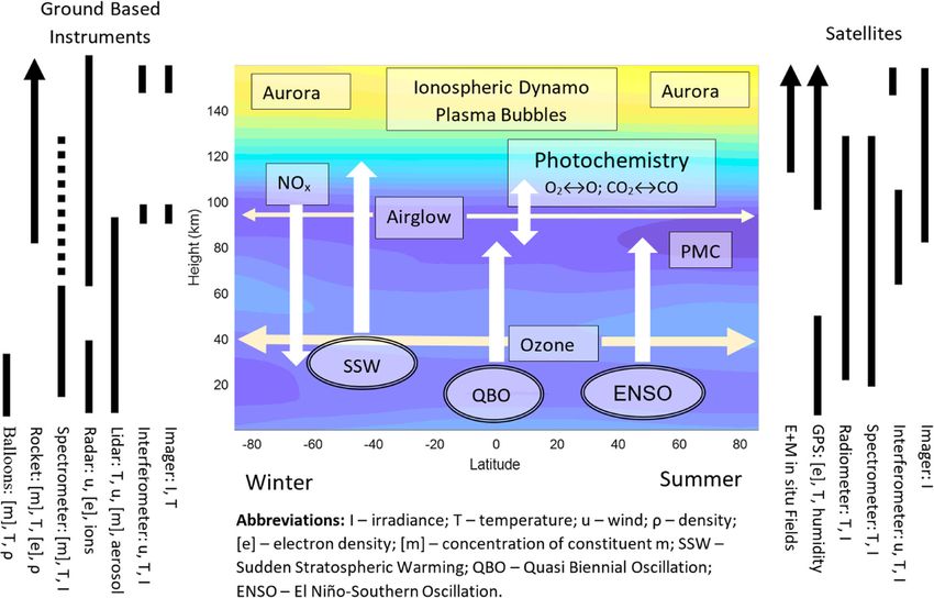
Ward et al. Progress in Earth and Planetary Science       (2021) 8:47                                                                        Page 5 of 38

 Fig. 2 The main drivers for coupling from above and below. The induced residual circulation is presented by white arrows. Black arrows represent
 the wave forcing and tides, as labeled. The color background represents the zonal mean temperature structure with blue indicating the coldest
 regions and yellow the warmest regions. The contour lines represent the zonal mean zonal wind structure (yellow is positive, i.e., eastward wind;
 dashed blue is negative, i.e. westward wind; black is the zero wind line). The radiative processes are in white, the elements of wave driving in orange,
 and downward particle precipitation in green

and/or temperature fields and their variability which allow                    coupling. The aurora is directly associated with downward
the strength and nature of the coupling processes to be                        fluxes of electrons along field lines and hence a signa-
investigated. Polar mesospheric clouds (PMC) appear in                         ture of downward influence. The ionospheric dynamo and
the summer upper mesosphere and are the result of up-                          plasma bubbles are ionospheric phenomena whose form
welling over the summer pole associated with the induced                       is influenced by upward propagating waves.
residual circulation. The photochemistry involves the                             The main terrestrial-associated solar-terrestrial cou-
cycling of constituents from the well-mixed lower atmo-                        pling components, namely energetic particle precipita-
sphere into the thermosphere where they are dissociated                        tion, solar irradiance absorption, and coupling associ-
and then diffuse downward to the mesosphere where they                         ated with waves and constituent transport, are summa-
recombine to form the original molecular species. The                          rized briefly below. This serves as an introduction to the
cycling between molecular and atomic oxygen is partic-                         more detailed review of recent progress which follows.
ularly important for the formation of the airglow which                        Of importance during the ROSMIC project was facilitat-
provides an important means of probing the dynamics of                         ing work which helped clarify the role and importance
the mesopause region. Ozone is a constituent whose dis-                        of these various processes in the atmosphere/ionosphere
tribution depends on photochemistry and transport. The                         response to solar variability. Also of importance was work
downward transport of NOx which affects ozone chem-                            being undertaken to model and assimilate space weather
istry is one of the significant mechanisms of downward                         effects on the ionosphere and thermosphere. This topic is
Ward et al. Progress in Earth and Planetary Science         (2021) 8:47                                                                         Page 6 of 38

 Fig. 3 Overview of the MALTI phenomena. The schematic summarizes the phenomena/processes of importance to the coupling processes in the
 MALTI as well as ground based (left side of figure) and satellite observation techniques (right side of figure) and their altitude extent. Ovals identify
 significant sources of internal atmospheric variability, and squares, phenomena of importance. Vertical arrows represent the height range, and
 horizontal arrows, the latitude range over which the phenomena/processes have influence

not reviewed in this paper, but the interested reader can                       which mainly impact the troposphere; here, the reader
find a review of the current capabilities in Scherliess et al.                  is directed to the recent comprehensive review article by
(2019).                                                                         Mironova et al. (2015).
                                                                                   The process of all these particles interacting with the
2.1 Energetic particles                                                         atmosphere is known as energetic particle precipitation,
Energetic charged particles, mainly electrons and pro-                          or EPP. As a result of EPP, whether of protons or elec-
tons from the Sun and the Earth’s magnetosphere, deposit                        trons, ionization is enhanced, leading to production of
energy into the atmosphere, particularly in the polar                           odd-hydrogen (HOx = H + OH + HO2 ) and odd-nitrogen
regions (see Fig. 2), where the particles are guided by                         (NOx = NO + NO2 ) in the middle atmosphere. As
the Earth’s magnetic field. Solar protons, ejected from the                     these are both known catalysts in ozone loss reactions,
Sun, typically have energies between about 1 MeV to a few                       solar influence via variations in EPP levels has implica-
hundred MeV and have direct access to the high polar lati-                      tions to both atmospheric chemical and radiative balance
tude middle atmosphere during solar proton events (SPEs)                        hence potentially affecting surface climate via downward
as shown in Fig. 4 (Seppälä et al. 2014). This range of                         coupling of introduced wind anomalies (Seppälä et al.
energies means that they can directly impact the altitudes                      2013). HOx is chemically short lived and thus so are
from the stratosphere to mesosphere. Energetic electrons,                       its atmospheric impacts. In contrast, NOx produced by
with auroral electrons with energies less than 10 keV, and                      EPP (known as “EPP-NOx ”) in the middle atmosphere is
medium energy electrons with energies from tens of keV                          mainly destroyed by photolysis and so has a long chemi-
up to a few MeV, originate in the magnetosphere and as a                        cal lifetime during polar winter. It is therefore subject to
result of magnetospheric processes, enter the atmosphere                        transport by the downward circulation over the winter
near the auroral ovals (as shown in Fig. 4). Note that                          pole. One of the challenges with estimating EPP effects is
we will not explicitly cover galactic cosmic rays (GCR),                        that, while good observations on proton fluxes and energy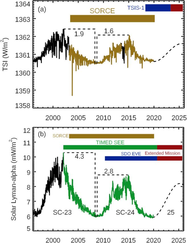
Ward et al. Progress in Earth and Planetary Science      (2021) 8:47                                                                      Page 7 of 38

 Fig. 4 Sources of EPP. The so-called medium energy electrons (MEE, > 10 keV to several MeV) originate in the Earth’s outer radiation belt, and their
 fluxes into the atmosphere are understood to be controlled by magnetospheric wave-particle interactions. Auroral electrons (< 10 keV) originate
 primarily from the plasma sheet which is located in the tail/night side of the magnetosphere, while solar protons (not included in the top image) are
 injected as a result of solar storms. The map in the bottom panel illustrates that the different types of particles can influence slightly different
 geographic areas when they enter the atmosphere (note that locations are only indicative and are influenced by the particle energies). While the
 Northern Hemisphere is shown here, precipitation also occurs in the Southern Hemisphere. For detailed information, see Matthes et al. (2017)

spectra during the large but sporadic SPEs exist, the limi-                  the Earth’s albedo (fraction of radiation reflected back
tations in electron observations have long hindered good                     to space), and outgoing long-wave infrared radiation that
characterization of both flux and energy spectrum of pre-                    can be altered by greenhouse gases, clouds, and aerosols.
cipitating electrons. Unlike solar radiation, there is not                   Changes in solar irradiance have both direct and indi-
a clear relation to the 11-year solar cycle, and the role                    rect effects on the Earth climate system, and the roles
of magnetospheric processes (such as those addressed in                      of solar irradiance are evident in many climate records
the VarSITI SPeCIMEN project) in electron precipitation                      (e.g., Solanki et al. (2013); Ermolli et al. (2013); Lean et
provides another challenge in their quantification.                          al. (2005)). There are two dominant direct solar heating
                                                                             effects in the lower atmosphere: the “bottom-up” mech-
2.2 Solar irradiance variability                                             anism is the solar irradiance warming the Earth’s surface
Solar radiation is the dominant energy input to the Earth                    and upward coupling, and the “top-down” mechanism
system with about 70% absorbed by the atmosphere, land,                      whereby solar ultraviolet radiation absorbed in the strato-
and ocean, and the remainder scattered and reflected                         sphere couples downward. The winds and circulations
back to space (L’Ecuyer et al. 2015). This energy partially                  in the atmosphere and oceans invoke complicated feed-
determines the temperature and structure of the atmo-                        backs that introduce non-linear and non-local responses
sphere and warms the Earth surface. Globally, a delicate                     (e.g., Meehl et al. (2008)). The solar radiation is also criti-
balance is maintained between incoming solar radiation,                      cally important in the Earth’s upper atmosphere. The solar
Ward et al. Progress in Earth and Planetary Science   (2021) 8:47                                                    Page 8 of 38

vacuum ultraviolet (VUV: shorter than 200 nm) photons               2.3 Transport and upward coupling through waves
originate in the Sun’s chromosphere, transition region,             The details of the chemistry and dynamics underlying the
and corona and deposit their energy in the Earth’s iono-            zonal mean structure of the stratosphere and mesosphere
sphere, mesosphere, and thermosphere, being regions                 and its variability have been recently reviewed by Baldwin
strongly influenced by space weather events like solar              et al. (2018). Much of the structure of the middle atmo-
flares.                                                             sphere is due to a combination of radiative forcing and
   A well-known example of the non-linear response of               transport of momentum and constituents by mean flows
the atmosphere to solar forcing (and an example of how              (i.e., the residual circulation) and mixing which are driven
the atmosphere modulates solar forcing) is what has been            in part by a broad spectrum of atmospheric waves. In
termed the natural “thermostat” effect (Mlynczak et al.             the middle atmosphere, the combined effect of the resid-
2003). During periods of enhanced geomagnetic effects               ual circulation and mixing is now starting to be termed
(coronal mass ejections and particle precipitation) and             the Brewer-Dobson circulation (Baldwin et al. 2018). The
variations in solar irradiance, the production of NO and            current consensus is that the Brewer-Dobson circulation
the associated near-infra-red cooling is enhanced. As               will be enhanced as a result of climate change. However,
these events are also associated with enhanced heating of           because of the complexities of the linkages between the
the atmosphere, the enhanced cooling serves to reduce the           different components identified in Fig. 1, exact drivers of
temperature response of the lower thermosphere to these             this change remain difficult to determine (Butchart 2014).
inputs. The extent to which this process influences the                The situation in the upper mesosphere and lower ther-
cooling was described using 12 years of SABER observa-              mosphere remains less studied and understood. Recent
tions by Mlynczak et al. (2014). Recent refinements to our          advances in our knowledge of sudden stratospheric warm-
understanding of this cooling process appeared in studies           ings reveal that the various regions of the atmosphere are
by Knipp et al. (2017) and Nischal et al. (2019).                   closely coupled. The associated wave dissipation in the
   The solar irradiance varies on all time scales with the          polar stratosphere not only influences the state of the mid-
key variations being the 11-year solar activity cycle (22-          dle atmosphere but drives global changes to the state of
year magnetic cycle), the 27-day solar rotation variability,        the thermosphere and ionosphere (Pedatella et al. 2018a).
and short-term (seconds to hours) variability during solar          Nevertheless, details of the mechanisms which main-
flares. The solar variability is highly dependent on wave-          tain the average conditions above the stratopause remain
length, which is related to the source regions in the solar         poorly understood. Wave dissipation in the mesosphere
atmosphere. The total solar irradiance (TSI: integrated             is considered important for the cycling of air through
over all wavelengths) and the solar spectral irradiance             the stratosphere and mesosphere and associated age of
(SSI) in the near ultraviolet (NUV, 300–400 nm), visi-              air calculations (see for example Kovács et al. (2017)).
ble (VIS, 400–800 nm), and near infrared (NIR, 800–                 The cycling of constituents and associated photochem-
3000 nm) comprises the bulk of the solar radiative energy           istry across the mesopause region is still being examined
and vary the least amount at about 0.1% over the 11-year            in terms of global temporal means (Garcia et al. 2014;
solar cycle and typically have less variability for shorter         Gardner et al. 2019; Swenson et al. 2018) as opposed to
time scales (e.g., Woods et al. (2018); Lean et al. (2005)).        zonal means or regional averages. There is indirect evi-
These NUV-VIS-NIR wavelengths are most important for                dence of a wave dissipation-driven, lower thermosphere
climate studies for assessing the influence of the Sun on           winter pole to summer pole circulation (opposite in direc-
Earth and for comparison with other natural processes               tion to the better known residual circulation in the middle
(such as volcanic eruptions and the El Niño Southern                atmosphere) (Qian et al. 2017; Qian and Yue 2017) which
Oscillation) and human activity (such as greenhouse gas             provides some indication of zonal mean structures at
production from fossil fuel combustion). The SSI is much            these heights. Apart from this, there is little information
more variable in the ultraviolet (UV) ranges: middle ultra-         on the seasonal variation and latitudinal structures of con-
violet (MUV; 200–300 nm), far ultraviolet (FUV; 120–                stituents and dynamics at these heights. This remains an
200 nm), extreme ultraviolet (EUV; 10–120 nm), and soft             important topic for future research.
X-rays (SXR, 0.1–10 nm) but involves only 1.5% of the                  The source of the wave activity is predominantly in
solar radiative energy. The solar cycle variability in the UV       the troposphere. As the waves propagate upwards, they
is less than 15% for MUV wavelengths, about a factor of             interact with the mean wind and temperature fields,
two for many EUV and FUV wavelengths, and even to fac-              which influence their propagation and dissipation, and in
tors of more than a 1000 for most SXR wavelengths (e.g.,            turn, the stress associated with wave dissipation modi-
Woods et al. (2018); Woods and Rottman (2002)). These               fies the global fields. These wave processes are therefore
UV ranges are most important for atmospheric research               non-linear and non-local. The nature of the wave field
and for space weather studies and applications involving            as a function of height was explored in detail in gen-
satellite operations, communications, and navigation.               eral circulation models of sufficient resolution and height
Ward et al. Progress in Earth and Planetary Science   (2021) 8:47                                                    Page 9 of 38

(Shepherd et al. 2000; Koshyk and Hamilton 2001; Hamil-             3.1 Progress and challenges in modeling
ton et al. 2008). They noted that the rotational compo-             Various advances have been made in both improving
nents dominated the kinetic energy spectrum lower in                modeling capability and identifying current limitations
the atmosphere with the divergent component becom-                  and future requirements. Reviews that contain details and
ing stronger with height and in the mesosphere becoming             insights to atmospheric modeling have recently been pub-
as strong as the rotational component. The divergent                lished by, e.g., Baldwin et al. (2018); Maher et al. (2019).
component is associated with atmospheric tides and grav-               One issue of importance to modeling is the influence
ity waves. Their increased relative importance above the            of solar UV irradiance on climate variability. Chiodo and
stratopause is reflected in the extensive literature devoted        Polvani (2016) addressed the limitations arising from the
to exploring gravity wave effects throughout the middle             assessments of this influence when interactive (coupled)
and upper atmosphere (and references therein Liu et al.             stratospheric ozone chemistry is not included. Model
(2014b); Yiğit and Medvedev (2015); Liu et al. (2017);             integrations with coupled chemistry are computationally
Becker and Vadas (2018); Miyoshi and Yiğit (2019)). Of             expensive. For example, the WACCM (Whole Atmo-
particular interest in these investigations is the analysis of      sphere Community Climate Model) model has a through-
SSWs as they provide the means to investigate structural            put of 7.5 simulated years/day on the US–based Yellow-
differences in wave forcing and propagation for conditions          stone supercomputer (Smith et al. 2014) with interactive
which deviate significantly from normal (Manney et al.              stratospheric chemistry. This is increased to 14.8 sim-
2009; Goncharenko et al. 2013; Ern et al. 2016; Siddiqui            ulated years/day with specified (non-interactive) chem-
et al. 2017; Pedatella et al. 2018b). The character of the          istry with the same number of CPUs (central processing
waves penetrating and affecting the ionosphere and ther-            unit), nearly a doubling of performance. Thus, for bet-
mosphere is a topic that is of significant current interest         ter computational efficiency, interactive chemistry is often
and continues to evolve. The waves of interest and some             omitted. Chiodo and Polvani (2016) showed that inclu-
of their characteristics are summarized by Liu (2016), and          sion of interactive stratospheric ozone chemistry reduces
the density variations associated with various atmosphere           the surface warming signal from solar irradiance signif-
and ionospheric phenomena are summarized in Liu et al.              icantly, by a third, when contrasted to predictions from
(2017).                                                             non-interactive (specified) chemistry. They conclude that
                                                                    models that do not take into account the responses in
3 Coupling from above                                               stratospheric chemistry are likely overestimating the sur-
This section will focus on the aspects of coupling from             face level response to solar variability.
above via solar forcing on the atmosphere and climate                  Another issue of importance is the credibility of
system. We will address EPP and solar irradiance sep-               model representations of the downward coupling of EPP-
arately. As there have been significant advances on the             induced chemical responses. The multi-model, multi-
modeling capability that impact both, we will first address         satellite intercomparison work of Funke et al. (2017)
the latest progress in modeling during the VarSITI period           examined how well various medium-top (model top lid
and briefly discuss some remaining challenges. In this              at about ∼ 80 km) and high-top (model top lid above
context, the earlier works of Gray et al. (2010) and                120 km) models performed in this capacity. They exam-
Seppälä et al. (2014) outline the progress on the topic             ined the ability of these models to reproduce polar down-
of solar influence on climate, as a result of previous              ward transport of high-altitude carbon monoxide and
SCOSTEP science programs. Many of the data sets impor-              odd nitrogen (NOx = NO + NO2 ) as well as observed
tant to this area are from satellite missions that are              middle atmosphere temperatures during a dynamically
no longer active. The lack of planned future missions,              perturbed Northern Hemispheric (NH) winter. The mod-
important for validating models and new ideas on the                els performed reasonably well until the polar vortex was
nature of this coupling, is of considerable concern to the          disrupted by a SSW event. These events frequently occur
community.                                                          in the Northern Hemisphere causing major disturbances
  The key questions initially identified by the Working             to the dynamical state of the atmosphere. They lead to
Group on Solar Influence on Climate were as follows:                the mixing of air masses and, sometimes, in the recov-
                                                                    ery phase, a reformation of the stratopause at typically
  1. Drivers of solar variability: How well do we know              mesospheric altitudes. These latter events are known as
     their magnitude and variability?                               elevated stratopause (ES) events and can result in effec-
  2. Mechanisms and coupling processes: How is the                  tive transport from the mesosphere and lower thermo-
     solar signal transferred down to the troposphere and           sphere (MLT) into the stratosphere (see also discussion in
     surface?                                                       Section 4).
  3. Solar influence on climate: What are the                          The descent of air masses as the newly formed
     uncertainties in establishing the long-term effect?            stratopause moves downwards to 50 km is challenging for
Ward et al. Progress in Earth and Planetary Science (2021) 8:47 Page 10 of 38 models to reproduce, with most simulating a too rapid partitioning of nitrogen compounds (Andersson et al. return of the stratopause to its typical height. Funke et al. 2016; Funke et al. 2017; Orsolini et al. 2018). (2017) determined that model improvements are needed There has been an increased interest in the role of the to address the lack of dynamical representation of ES stratosphere in tropospheric variability and the poten- events. To date, the closest representation of the down- tial for improved predictions. While it still remains to ward descent following an ES event has required either be determined if stratospheric influence is relevant for relaxing (“nudging”) the model toward assimilated mete- daily weather forecasts (Baldwin et al. 2018), growing orological fields up to about the altitude of 90 km (Siskind evidence is supporting inclusions of stratospheric infor- et al. 2015), or the more self-consistent approach of using mation to produce skillful seasonal forecast from a few data assimilation in a chemistry climate model such as months to up to a year ahead (Thiéblemont et al. 2015; WACCM-DART (Pedatella et al. 2018b). This approach Dunstone et al. 2016). There are further indications that is only possible for times when meteorological observa- the ability to simulate stratospheric variability, whether in tions (and thus assimilated products) are available and the ozone, SSW occurrence or large-scale modes such as the models can be constrained to observed dynamics. The quasi-biennial oscillation (QBO) leads to improvements model improvements called on by Funke et al. (2017) elsewhere in the atmosphere/climate system (Baldwin et have not been fully implemented and remain necessary al. 2018). For the top-down coupling, this would sug- to improve the dynamical capabilities of atmospheric and gest that mesospheric and thermospheric chemical and climate models. dynamical processes contributing to stratospheric vari- Meraner et al. (2016) found that the parameterization ability also need to be investigated—one of the questions of non-orographic gravity waves played an important role to be addressed in PRESTO (Shiokawa and Georgieva in improved representation of the MLT to stratosphere 2021) is the predictability in sub-seasonal to decadal vari- descent following ES events in the Hamburg Model of the ability for the atmosphere and climate. Neutral and Ionized Atmosphere (HAMMONIA). Their results suggest that improvements to gravity wave param- 3.2 Energetic particle precipitation eterizations may need to be made to simulate realistic The widespread shift from SPE focused, event type studies downward transport brought on by ES events. As the (e.g., Funke et al. (2011)), toward more general considera- ES events can bring MLT air, rich in EPP-NOx , into the tion of EPP impacts on the atmosphere that we saw during stratosphere, Randall et al. (2015) further highlighted the the CAWSES-II program (Seppälä et al. 2014) has contin- need to have a realistic representation of energetic parti- ued during VarSITI. The current consensus is that EPP, cle precipitation (EPP) to bring down sufficient amount of in the form of EEP, modulated by magnetospheric activ- NOx into the stratosphere. ity, is an important driver for the chemical variability of The missing EPP contributions and the associated the polar middle atmosphere. This needs to be captured in underestimation of EPP-NOx in the polar mesosphere chemistry-climate models in order to correctly represent have lead to two significant developments in climate mod- natural polar ozone variability. Figure 4 illustrates some of eling during VarSITI. Firstly, we now have the first long- the key differences in the sources and impact areas of SPEs term energetic electron precipitation (EEP) dataset for and different types of EEP. use in climate modeling. This is now incorporated into In particular, Stone et al. (2018) highlighted the need to the recommended solar irradiance and energetic parti- account for SPEs when evaluating the recovery of strato- cle forcing for CMIP6 simulations (Matthes et al. 2017) spheric ozone due to chlorofluorocarbons (CFCs). SPEs and will be addressed further later in the Section 3.2. could have both direct (in situ) and indirect (via trans- The second major improvement is the development of ported EPP-NOx ) influences on stratospheric ozone. Den- the first fully coupled climate model with comprehensive ton et al. (2017; 2018) analyzed ozonesonde data from lower ionosphere (D-region) ion chemistry (307 reactions the NH polar region and found that, once seasonal back- of 20 positive ions and 21 negative ions) (Verronen et ground variability was taken into account, lower strato- al. 2016). This version of the WACCM model, the whole spheric ozone (altitudes below 35 km) was reduced in atmosphere component of the Community Earth System excess of 30 days from the start of the SPEs, with an Model (CESM), called WACCM-D enables detailed stud- average depletion of 5–10%. However, these results were ies of the global lower ionosphere and its response to recently disputed by Jia et al. (2020). external (e.g., solar) and internal (e.g., dynamical) forcing. As SPEs are only a fraction of the total EPP, it is likely WACCM-D includes fully interactive chemistry, radia- that further improvements on simulated ozone variabil- tion, and dynamics. For the purposes of EPP studies, the ity on decadal scales would arise from inclusion of EEP. inclusion of detailed ion chemistry leads to improved rep- This has been partially addressed by the development of resentation of production of NOx and HOx gases, by the first EEP proxy model for inclusion of ionization from removing the need for parameterizations, and the re- the so called “medium energy electrons” (with energies up
Ward et al. Progress in Earth and Planetary Science   (2021) 8:47                                                   Page 11 of 38

to 1 MeV) in climate models (van de Kamp et al. 2016;               from observations, nor is it clear to what extent these
Matthes et al. 2017; van de Kamp et al. 2018). As men-              types of electron precipitation are included in the existing
tioned earlier, this is now the official input to CMIP6             EEP proxy (Matthes et al. 2017).
model simulations going into IPCC AR6. Overall, the first              To capture the descent of MLT NOx into the strato-
EEP proxy is an underestimation of the total electron pre-          sphere, Funke et al. (2014b) analyzed 10 years of satel-
cipitation, and recent improvements to EEP observations             lite observations from the Michelson Interferometer for
(Peck et al. 2015; Nesse Tyssøy et al. 2016; Clilverd et            Passive Atmospheric Sounding (MIPAS) instrument on-
al. 2017; Oyama et al. 2017; Nesse Tyssøy et al. 2019)              board the Envisat satellite. The instrument simultane-
will likely further aid our understanding of variability in         ously measured several different middle atmosphere con-
this type of solar forcing into the atmosphere and lead to          stituents, enabling the extraction of purely EPP produced
inclusion of more accurate levels of EEP in model studies           reactive nitrogen, NOy , from the record. By the end of
(Smith-Johnsen et al. 2018).                                        the polar winter/start of spring, the descent of NOy into
  To test the van de Kamp et al. (2016) EEP model, Ander-           the stratosphere was observed to reach altitudes of 30 km
sson et al. (2018) ran simulations with the WACCM model             and below in the NH and 25 km and below in the SH
to investigate the impact of inclusion of electron pre-             during the time period studies. The results highlighted
cipitation on middle atmosphere chemistry. They found               the asymmetries between the two poles arising from the
that, on average, mesospheric ozone was reduced by up               very different dynamical conditions controlling the atmo-
to 20% by inclusion of the new EEP forcing, while in the            sphere in the north and the south: In the SH, Funke et
stratosphere, there was an additional 7% ozone loss when            al. (2014b) show a steady annual descent of EPP-NOy
contrasted to simulations without EEP. They further noted           from the mesosphere to the stratosphere inside the sta-
that on solar cycle scales, the inclusion of EEP in WACCM           ble SH polar vortex, with the overall amount of NOy
doubled the stratospheric ozone response. These results             depending on the solar cycle and level of geomagnetic
can be contrasted to the multi-satellite observations pre-          activity. In the NH, not only did the overall levels of NOy
sented by Andersson et al. (2014), who found that on                depend on the solar and geomagnetic activity, but also
solar cycle timescales, EEP can drive mesospheric ozone             the large dynamical variability present in the polar atmo-
variations of up to 34%.                                            sphere. SSW/ES events had a significant impact on the
  In their multi-satellite observational study, Damiani             descent rates as well as the amount and timing of the
et al. (2016) showed evidence that EPP in general has               NOy reaching the stratosphere. Funke et al. (2014a) use
influenced Antarctic upper stratospheric ozone since                these EPP-NOy observations to derive the total amount
1979, at a level of 10–15% O3 depletion on a monthly                of NOy molecules in the polar atmosphere reaching alti-
basis. This is slightly more than found by Fytterer et al.          tudes below 70 km. They found a nearly linear correlation
(2015), who estimated Antarctic ozone depletion of 5–               between the amount of NOy and the geomagnetic Ap
10% using observations from a different set of satellite            index for the winter period extending to early spring, con-
instruments. Using two independent chemistry-climate                firming earlier works by Randall et al. (2007); Seppälä et
models (CCMs), Arsenovic et al. (2019) and Pettit et al.            al. (2007), with the NH again showing large responses to
(2019) showed that only by including EEP were models                dynamical perturbations.
able to reproduce stratospheric ozone anomalies found                  Based on these findings from the MIPAS data set,
in satellite observations. A number of further studies              Funke et al. (2016) presented a semi-empirical, a p-driven,
(e.g., Zawedde et al. (2016); Smith-Johnsen et al. (2017);          proxy model for EPP-NOy descending though meso-
Smith-Johnsen et al. (2018); Newnham et al. (2018)) have            sphere and upper-stratosphere. The model provides a
demonstrated EEP impacts on both HOx and NOx gases.                 seasonal dependent flux of EPP-NOy descending through
  Together, these suggest that there is need to improve             given vertical levels. One of the main uses of this semi-
the EEP forcing (the current EEP proxies are known to               empirical model is as an upper boundary condition (UBC)
underestimate precipitating levels, see Nesse Tyssøy et             for chemistry-climate models to emulate the descent of
al. (2019)) to ensure better representation of ozone vari-          NOy rich air from the MLT region. For CMIP6, the rec-
ability in the middle atmosphere. A wider source of EEP             ommended way of taking into account production of
are also likely to influence ozone variability in the meso-         EPP-NOx above the upper boundary of medium-top mod-
sphere. Seppälä et al. (2015), Turunen et al. (2016), and           els is by employing the Funke et al. (2016) UBC (Matthes
Seppälä et al. (2018) investigated the potential impacts on         et al. 2017). Figure 5 outlines the different approaches of
mesospheric ozone levels from auroral substorms (which              inclusion of sources of EPP in model simulations.
are known to occur frequently), pulsating aurora, and the              Following from the work of Funke et al. (2014b), Gor-
more energetic relativistic electron microbursts, respec-           don (2020) recently showed evidence that not only can
tively. They found all to influence ozone levels by up to           EPP-NOx reach altitudes of 25 km and below by the end
tens of percent, but thus far, this has not been verified           of the Antarctic polar winter, but once in the stratosphere,
Ward et al. Progress in Earth and Planetary Science    (2021) 8:47                                                                 Page 12 of 38

 Fig. 5 CMIP6 recommendation for including EPP in model simulations. The different approaches for auroral energy electrons (< 10 keV), medium
 energy electrons (MEE), and solar proton events (SPE). For details, see Matthes et al. (2017)

it remains in the stratospheric NOx column throughout                       While the latest meteorological re-analysis investiga-
the spring until breakup of the SH polar vortex. They                     tions (e.g., Maliniemi et al. (2018); Salminen et al. (2019))
found that the role of EPP in the springtime Antarc-                      continue to suggest that there are important implications
tic stratospheric NOx column is modulated by the QBO.                     to atmospheric dynamical variability on decadal scales,
They proposed that as CFCs are reduced, EPP-NOx will                      the results from simulations with a range of CCMs are
likely take a larger role in Antarctic springtime ozone loss              somewhat inconclusive (Arsenovic et al. 2016; Meraner
processes.                                                                and Schmidt 2018; Sinnhuber et al. 2018), particularly
   As we see from above, there is a growing body of evi-                  when it comes to relevance of EPP forcing to surface level
dence that EPP plays an important role in atmospheric                     climate variability. However, importantly, results from the
chemical balance, extending to decadal scales. Including                  latest model studies by Arsenovic et al. (2016), and the
this source of variability in medium-top and high-top                     multi-model study by Sinnhuber et al. (2018) are in agree-
models is now possible for the first time due to develop-                 ment with earlier model investigations (Baumgaertner et
ment of the CMIP6 EPP forcing input and the EPP-NOx                       al. 2011), and also with earlier meteorological reanalysis
UBC (Matthes et al. 2017), but further improvements are                   studies (Seppälä et al. 2013). They found that inclusion
still needed. Questions remain unanswered at the end of                   of EPP resulted in changes in polar winter stratospheric
the VarSITI program: What is the exact size of the EEP-                   temperatures (Arsenovic et al. 2016) or radiative heat-
NOx source and how important is overall EPP-induced                       ing patterns (Sinnhuber et al. 2018). The Sinnhuber et al.
chemistry to climate variability?                                         (2018) study further found that state-of the-art models
Ward et al. Progress in Earth and Planetary Science (2021) 8:47 Page 13 of 38
accounting for EPP are able to reproduce observed chemi- long-term (solar cycle scales) and short-term, models of
cal effects. The introduced radiative forcing changes in the solar variability, and, finally, the atmospheric and climate
polar stratosphere are of a similar order to those caused impacts.
by UV variability in the tropics, however, with alternating
sign in mid winter (polar night) and spring. 3.3.1 Long-term variability—solar cycle
Recently, Maliniemi et al. (2020) addressed the benefit The nearly periodic 11-year solar cycle is manifested by
of accounting for the full description of the CMIP6 solar the regular presence of numerous large sunspots during
forcing (both irradiance and EPP) in future projections. By solar maximum and few, if any, sunspots during solar min-
looking at the amount of NOx descending into the strato- imum. These sunspots are the result of magnetic activity
sphere, they were able to conclude that climate change will rising up through the Sun’s photosphere. Three decades
likely increase the EEP-related atmospheric effects toward of space-based research document dramatic increases in
the end of the century. solar photon, particle, and plasma energy output accom-
panying the increase in sunspot numbers. Figure 6 shows
3.3 Solar irradiance that in the recent solar cycles 23 and 24, the TSI increased
This section will outline the recent progress in the during the maximum by about 0.14% relative to solar min-
understanding of variability in solar irradiance, in both imum and that the SSI H I Lyman-α emission at 121.6 nm
Fig. 6 Solar variability over solar cycles 23 and 24. Examples of solar variability over solar cycles (SC) 23 and 24 for a the total solar irradiance (TSI) and
b the bright ultraviolet H I 121.6 nm Lyman-α emission. The SORCE TSI observations shown here are being extended with TSIS-1 observations.
Important solar UV irradiance records over solar cycle (SC) 23 and 24 have been established with TIMED SEE observations, and the TIMED SEE and
SDO EVE observations will be extended into the next solar minimum and cycle 25. These extensions are particularly important for overlapping with
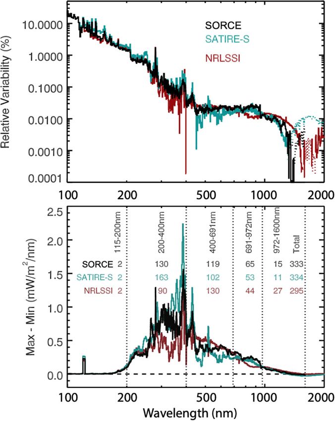
the new GOLD and ICON missions to observe the ionosphere-thermosphere during cycle 25Ward et al. Progress in Earth and Planetary Science (2021) 8:47 Page 14 of 38 increased by about a factor of 1.7 at maximum relative smaller than the measurement uncertainty and in the to minimum. It is also important to note the difference near infrared (NIR) where many wavelengths have out- in cycle maximums. In particular, the ratio of the solar of-phase (negative) variability over the solar cycle (e.g., variability, defined as maximum minus minimum, at cycle Ermolli et al. (2013)). The NASA Total and Solar Spec- 24 maximum to the variability in cycle 23 is 0.84 for TSI tral Irradiance Sensor (TSIS-1) observations that started and 0.65 for Lyman-α. Moreover, cycle 24 maximum has in 2018 are anticipated to address the SSI variability more proven to be the weakest during the past 90 years. accurately for the visible and NIR ranges. As described earlier, the SSI variability is very wave- The TSI at the 2008–2009 minimum also appears to length dependent. The solar cycle variability for the SSI as be lower by 0.2 W/m2 (− 140 ppm) than the previous a function of wavelength is shown in Fig. 7. These obser- minimum in 1996 (Fröhlich 2009); however, the 100 ppm vations are from NASA’s Solar Radiation and Climate uncertainty of this TSI change makes this finding less Experiment (SORCE (Rottman et al. 2005)), launched in certain (e.g., Kopp and Lean (2011)). Observations taken 2003 and also the Thermosphere Ionosphere Mesosphere during the next solar minimum in 2019–2020 will be Energetics and Dynamics (TIMED (Woods et al. 2005)) very intriguing in terms of determining whether the sec- spacecraft, launched in 2001. The exact amount of SSI ular trend of lower solar activity is continuing or not. variability from the SORCE mission is under debate pri- There are already some indications that the solar activ- marily in the visible where the amount of variability is ity could continue to decline as indicated from studying Fig. 7 SORCE solar spectral irradiance variability. The SORCE solar spectral irradiance variability results from Woods et al. (2015), shown in black, are compared to the SATIRE-S (blue) and NRLSSI (red) model estimates for solar variability between February 2002 (max) to December 2008 (min). The top panel shows the relative variability in percent, and the bottom panel shows the absolute variability in irradiance units. The dashed lines are out-of-phase (negative) solar cycle variability results. The irradiance variability (max-min) in broadbands is provided, and those numbers are in units of mW/m2 . The total variability is for the 115 to 1600 nm range. This figure is adapted from Woods et al. (2015)
You can also read