Scheduling the Brazilian OR Conference - Optimization Online
←
→
Page content transcription
If your browser does not render page correctly, please read the page content below

Scheduling the Brazilian OR Conference
Rubens Correia1 , Anand Subramanian1 , Teobaldo Bulhões1 , and Puca Huachi V. Penna2
1
  Universidade Federal da Paraı́ba, Centro de Informática, Rua dos Escoteiros, s/n Mangabeira, João Pessoa–PB, Brazil
2
  Universidade Federal de Ouro Preto, Departamento de Computação, Instituto de Ciências Exatas e Biológicas, Campus
                           universitário – Morro do Cruzeiro, 35400-000, Ouro Preto, Brazil

                                               January 13, 2021

                                                      Abstract

         In this paper, we show how to efficiently schedule the Brazilian OR conference using a matheuristic
      approach. The event has traditionally around 300 presentations across a period of 3 to 4 days, and
      building a schedule for the technical sessions is an arduous task. The proposed algorithm integrates
      the concepts of iterated local search and simulated annealing with two mathematical programming-
      based procedures. The idea is to first group the presentations via a clustering procedure, and handle
      the side constraints in a subproblem via an integer programming formulation. A set partitioning
      procedure is applied at the end of the algorithm to find the optimal combination of clusters found
      during the search. We first assess the performance of the method by comparing our results with the
      dual bounds attained in the literature on two existing sets of artificial instances derived from other two
      conferences. Next, we executed our approach on the real-life instances derived from different SBPO
      editions, and compared the solutions with the manual solutions, when available, or with dual bounds
      found by an exact algorithm from the literature. The results obtained show that the matheuristic is
      capable of achieving high quality solutions both on the artificial and real-life instances.

1    Introduction
The Brazilian Operations Research (OR) conference, officially called Simpósio Brasileiro
de Pesquisa Operaiconal (SBPO), is an event organized every year by the Brazilian OR
society, formally known as Sociedade Brasileira de Pesquisa Operacional (SOBRAPO).
SBPO has now reached more than 50 editions, and it is considered the main national OR
conference, gathering hundreds of participants, from undergraduate students to practi-
tioners and experienced researchers.
   The event follows the format of a typical academic conference by including technical
sessions, plenary talks, short-term courses, poster sessions, social activities, and so on,
during a period of 4 days. We are particularly interested in solving the problem of

                                                          1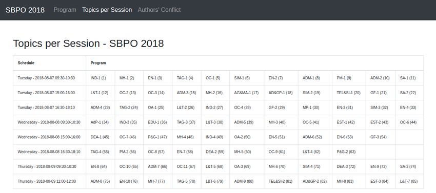
scheduling the presentations of technical sessions, which is by far the most challenging
task for the organizers. The other activities can be easily scheduled without much effort.
   Up to 2018, the problem was solved manually during several days, and finding high
quality solutions was viewed as an arduous task. The initiative of addressing the problem
using an optimization approach started that year, and it continues to be used to this
date. In this paper, we describe in detail the strategy developed for successfully solving
the problem.
   The scheduling criteria specified by the SBPO organizers fit precisely the generic
clustering-based model recently introduced by Bulhões et al. [2020] for conference schedul-
ing (CS) problems. Nevertheless, the exact algorithm proposed by the authors was not
capable of solving all of the real-life instances (with up to 324 presentations) derived
from the referred event to optimality in an acceptable CPU time. Therefore, the main
contribution of this work is the development of an efficient matheuristic algorithm that
combines the principles of iterated local search (ILS) and simulated annealing (SA) with
two mathematical programming-based procedures. The idea is to group the presentations
with similar topics in a same session using a clustering procedure based on ILS and SA,
and then handle the side constraints in a subproblem via an integer linear programming
(ILP) formulation. A set partitioning procedure is applied at the end of the algorithm as
an attempt to find the optimal combination of clusters found during the search.
   We first evaluate the performance of the matheuristic by means of extensive computa-
tional experiments on artificial benchmark instances derived from two other conferences,
and compare the results obtained by our method with the existing dual bounds produced
by the exact procedure devised in Bulhões et al. [2020]. We then compare the results
found by our approach on real-life instances derived from SBPO with the manual solu-
tions, or with the dual bounds provided by the exact algorithm, in order to confirm the
high performance of the proposed algorithm. Moreover, we believe that the matheuristic
devised in this work can be either directly applied or easily adapted to solve a wide range
of CS problems.
   The remainder of the paper is structured as follows. Section 2 presents a brief liter-
ature review. Section 3 formally defines the problem. Section 4 describes the proposed
algorithm. Section 5 contains the results of the computational experiments. Section 6
concludes.

                                             2
2 Related work
The literature on CS dates back more than 30 years. Eglese and Rand [1987] were one of
the first to study the problem by trying to maximize the preference of the participants.
They proposed a formulation and a two-phase heuristic. Sampson and Weiss [1995] ad-
dressed an extended version of the problem by considering the capacity of the rooms. A
heuristic procedure was developed by the authors, that was also later used to examine
the influence of some factors (e.g., conference length) on the resulting schedule [Sampson
and Weiss, 1996]. Le Page [1996] devised a heuristic procedure for a CS problem that
aims at minimizing the conflicts of presentations assigned to parallel sessions based on
the preference of the attendees.
Thompson [2002] also studied a variant of the model suggested in Eglese and Rand
[1987] by assuming the existence of rooms with different capacities, and they put forward a
SA algorithm. Sampson [2004] later compared the preference-based CS with other related
problems, namely course timetabling and exam timetabling. The author also modified the
original model by Eglese and Rand [1987], and devised a SA approach for the problem.
Gulati and Sengupta [2004] developed a heuristic for a extended version of the model pre-
sented in Sampson [2004], which incorporated other criteria, namely reviewer evaluations
and session times.
Mori and Tanaka [2002], Tanaka et al. [2002] tackled a CS problem with the objective
of grouping the most similar works in a same session. The former proposed a genetic
algorithm, the latter a so-called self organizing map, which is based on the concept of
unsupervised neural network. Potthoff and Munger [2003] addressed the problem of as-
signing sessions containing 3 or 4 presentations, defined a priori, to time slots. They also
assumed that a presenter can perform other roles such as the coordinator (a.k.a. chair)
of the session. Therefore, one must ensure that he/she cannot be assigned to parallel
sessions. A mixed integer programming (MIP) formulation was proposed, which was used
to schedule the Annual Meeting of the Public Choice Society of 2001. Potthoff and Brams
[2007] later applied the same method to schedule the 2005 and 2006 editions of the same
conference but this time considering the availability of the presenters.
Nicholls [2007] implemented a heuristic for a CS problem that attempt to satisfy the
preferences of the presenters, whereas Ibrahim et al. [2008] applied combinatorial design
results to generate a balanced schedule. Edis and Sancar Edis [2013] proposed a model
that tries to optimize two objectives: (i) minimize the number of parallel sessions with
presentations of the same topic; and (ii) balance the number of presentations of the parallel
sessions. Quesnelle and Steffy [2015] developed a model to minimize attendee preference
3conflicts that also avoids presentations by a same author to be assigned to parallel sessions.
Rahim et al. [2017] implemented a so-called domain transformation approach to solve a
problem with a similar preference-based objective.
Vangerven et al. [2018] solved a CS problem aiming at maximizing the attendees’
preference and minimizing the number of hops, i.e., the number of times a participant
has to change rooms to attend a presentation of his/her interest. The authors proposed
a three-phase algorithm based on integer programming and heuristics to solve four real-
life conferences. Stidsen et al. [2018] addressed the problem of scheduling the EURO-k
conferences by solving five MIP models sequentially. The problem has several objectives
to cope with the hierarchical structure of the conference.
Finally, Bulhões et al. [2020] proposed a clustering-based approach to model CS con-
ferences in general. The idea is to group the presentations according to their level of
similarity and handle the specificities of the conference by means of side constraints.
They proposed three exact approaches: (i) a compact integer programming formulation;
(ii) an alternative formulation, in which lazy cuts are added on demand in case any of the
side constraints is violated; and (iii) a branch-cut-and-price algorithm over a set partition-
ing (SP) formulation. They reported results for real-life and artificial instances derived
from two conferences.
3 Problem definition
Historically, the organizers of SBPO have been grouping similar papers into a thematic
session (e.g., “Combinatorial Optimization”, “Metaheuristics”, etc.), and this format has
been well accepted by the participants. Moreover, they usually tend to avoid parallel
sessions with similar topics, as well as many sessions of a similar topic to occur in a
same day. They also try to avoid papers from a same author to be scheduled in parallel
sessions. Other particularities such as presenter’s availability are handled a posteriori,
once a scheduled has been built. The optimization problem defined in this section was
modeled exactly as specified by the organizers. We first introduce some notation, and
then we formally provide the objective function and constraints of the problem.
We are given the following sets:
• P = {1, . . . , n} – set of papers (or presentations);
• D – set of days;
• H – a set of non-overlapping time slots;
4• S – set of sessions;
• T – set of topics;
• A – set of authors;
• Pa ⊆ P – set of papers by author a ∈ A;
• Pt ⊆ P – set of papers associated with topic t ∈ T ;
• Tj ⊆ T – set of topics of paper j ∈ P ;
• Aj ⊆ A – set of authors of paper j ∈ P .
In addition, we denote by ds and hs the day and the time slot of session s ∈ S, respectively;
and we define the following additional sets:
• Sd = {s ∈ S : ds = d} set of sessions of day d ∈ D;
• Sh = {s ∈ S : hs = h} set of sessions of time slot h ∈ H;
• Sdh = {s ∈ S : ds = d ∧ hs = h} set of parallel sessions of day d ∈ D and time slot
h ∈ H.
Each pair of distinct papers i, j ∈ P has an associated unrestricted benefit bij ∈ R if
both are assigned to a same session. The higher the number of common topics in both
papers, the higher the benefit. Each paper has at most three topics. The objective of the
problem is to maximize the total benefit, subject to the following constraints: (i) each
paper i ∈ P must be assigned to exactly one session s ∈ S; (ii) a non-empty session s ∈ S
must have at least ms papers and at most Ms papers; (iii) there cannot be more than one
paper i ∈ P by a same author a ∈ A assigned to parallel sessions; (iv) there should be at
most MD papers associated with topic t ∈ T per day; and (v) there should at most MH
papers associated with topic t ∈ T assigned to time slot h ∈ H on the same day d ∈ D,
regardless of the session.
Constraints (i)–(ii) can be seen as basic constraints, whereas constraints (iii)–(v) are
assumed to be side constraints. The last constraint was specifically imposed by the
SBPO organizers in order to prevent various papers with the same topic to be scheduled
in parallel sessions. The remaining constraints were defined in Bulhões et al. [2020], along
with the proof of N P-hardness.
Given a feasible solution, the order of presentations of each session can be arbitrarily
defined. The topic of the session is defined as the mode of the topics of the associated
papers.
54 Proposed algorithm
The outline of the proposed multi-start algorithm, denoted as HILS, is presented in Algo-
rithm 1. At each of the IR restarts (lines 6–39), HILS tries to improve the initial solution,
generated via a greedy randomized procedure (line 7), by iteratively performing local
search (line 13) and perturbation (line 35) moves for at most IILS consecutive iterations
without improvements (lines 12–38).
Algorithm 1 HILS
1: Procedure HILS(IR , IILS , τ0 , α)
2: f ∗ ← 0 . Objective value of the best feasible solution
3: s∗ ← ∅ . Best feasible solution
4: ClusterP ool ← ∅
5: SolutionM emory ← ∅
6: for i := 1 to IR do
7: s ← GenerateInitialSolution()
8: s0 ← s
9: s00 ← s
10: iterILS ← 0
11: τ ← τ0
12: while iterILS ≤ IILS do
13: s ← LocalSearch(s)
14: if s ∈/ SolutionM emory then
15: ClusterP ool ← UpdateClusterPool(s, ClusterP ool)
16: SolutionM emory ← UptadeSolutionMemory(s)
17: if f (s) > f ∗ and CheckFeasibility(s) = true then
18: s∗ ← s
19: f ∗ ← f (s)
20: end if
21: end if
22: ∆ ← f (s) − f (s0 )
23: if ∆ > 0 then
24: s0 ← s
25: s00 ← s
26: iterILS ← 0
27: else
28: select x ∈ [0, 1] at random
29: if τ > 0 and x < e−∆/τ then
30: s0 ← s
31: else
32: s0 ← s00
33: end if
34: end if
35: s ← Perturb(s0 )
36: iterILS ← iterILS + 1
37: τ ←τ ×α
38: end while
39: end for
40: s∗ ← SP(s∗ , ClusterP ool)
41: return s∗
42: end HILS.
6Each solution can be seen as a collection of clusters. A cluster contains the presen-
tations of a session. Hence, for each session, there is an associated cluster with a given
minimum and maximum limit of papers. The clusters from local optimal solutions are
stored in a pool (line 15). Such solutions are also stored along with their respective ob-
jective values in a structure denoted as SolutionMemory (line 16). In case one of these
solutions is found again, the local search is interrupted and the corresponding solution is
returned as the current local optimum.
At the end of each local search, the algorithm checks if the solution belongs to Solu-
tionMemory. If so, one verifies whether such solution satisfies the side constraints (lines
17–19) using an ILP formulation (see Section 4.1). If so, then the best feasible solution
s∗ is updated.
The criterion used to select the local optimal solution to be perturbed is based on SA
(lines 29–33). Parameter τ is initialized at each restart with τ0 (line 11), and its value
decreases at each iteration according to a factor α ∈ [0, 1] (line 37). The smaller the value
of τ , the smaller the probability (line 29) of accepting a non-incumbent local optimum
as the next solution to be perturbed. When the non-incumbent solution is not accepted,
the algorithm restores the current incumbent solution for applying the perturbation (line
32).
Finally, at the end of the procedure, the algorithm attempts to find the optimal com-
bination of clusters from the pool with a view of finding an improved solution (line 40).
This is done by an exact approach based on set partitioning (SP) (see Section 4.2).
4.1 Feasibility checking
Define C = {C1 , C2 , . . . , Cl } as a collection of clusters from a given solution, from which
we can derive the following sets:
• Ca ⊆ C – set of clusters containing the papers by author a ∈ A;
• Sj ⊆ S – set of sessions that cluster Cj ∈ C can be assigned to.
The amount of papers of cluster Cj ∈ C associated with topic t ∈ T is denoted by Qtj .
Moreover, let the binary variable xsj assume value 1 if cluster Cj ∈ C is assigned to session
s ∈ S, 0 otherwise. We can write the model for checking feasibility as follows.
Min 0 (1)
7Subject to:
X
xsj = 1, ∀Cj ∈ C (2)
s∈Sj
X
xsj ≤ 1, ∀s ∈ S (3)
Cj ∈C:s∈Sj
X X
xsj ≤ 1, ∀a ∈ A, ∀d ∈ D, ∀h ∈ H (4)
Cj ∈Ca s∈S h ∩Sj
d
X X
Qtj xsj ≤ MD , ∀t ∈ T, ∀d ∈ D (5)
Cj ∈C s∈Sd ∩Sj
X X
Qtj xsj ≤ MH , ∀t ∈ T, ∀d ∈ D, ∀h ∈ H (6)
Cj ∈C s∈Sdh ∩Sj
xsj ∈ {0, 1}, ∀Cj ∈ C, ∀s ∈ Sj . (7)
Constraints (2) ensure that each cluster must be assign to exactly one session. Con-
straints (3) guarantee that at most one cluster is assigned to a session. Constraints (4)
avoid papers from a same author to be assigned to parallel sessions. Constraints (5) and
(6) impose a limit on the amount of papers from a same topic to be assigned in the same
day and time slot, respectively. Finally, constraints (7) define the domain of the decision
variables.
4.2 Set partitioning approach
Given a pool of clusters, we can define the following sets:
• C – set of clusters;
• K – set of session sizes;
• Ci – set of clusters containing paper i ∈ P ;
• Sk – set of sessions of size k ∈ K;
• Ck – set of clusters that can be assigned to a session of size k ∈ K.
Let b0j be the benefit of a cluster j ∈ C. Define yj as a binary variable that assumes
value 1 if cluster j ∈ C is selected, and 0 otherwise. The SP formulation can be expressed
as follows.
X
Max b0j yj (8)
j∈C
8Subject to:
X
yj = 1, ∀i ∈ P (9)
j∈Ci
X
yj ≤ Sk , ∀k ∈ K (10)
j∈Ck
yj ∈ {0, 1}, ∀j ∈ C. (11)
Objective function (8) maximizes the total benefit. Constraints (9) are the partitioning
constraints, i.e., they guarantee that each paper is assigned to exactly one cluster. Con-
straints (10) impose a limit on the number of clusters of size k ∈ K that can be selected.
Constraints (11) define the domain of the variables.
The formulation given by (8)–(11) is incomplete because it does not include the side
constraints. Therefore, we implemented a branch-and-cut algorithm with a lazy separation
procedure, that is, every time an incumbent solution is found, the procedure verifies its
feasibility using the model described in Section 4.1, and add a lazy cut to remove infeasible
solutions.
4.3 Constructive procedure
The constructive procedure works as follows. Initially, a random paper is assigned to each
cluster. The remaining papers are iteratively inserted in a greedy fashion, more precisely,
the best insertion is the one that yields the highest increase in the objective function.
After all papers are inserted, the procedure verifies if there are clusters that violate the
minimum limit of papers. If so, the papers from such clusters are removed from the
partial solution, and the algorithm tries to reinsert them in other clusters. If it is still not
possible to build a feasible solution, the papers that could not be reinserted are relocated
to a dummy cluster with negative benefit, which is naturally emptied during the local
search.
4.4 Local search
Two neighborhood structures are employed during the local search, namely:
• Relocate (N (1) ) – one paper from a cluster is relocated to another one. Only feasible
moves are considered;
• Swap (N (2) ) – two papers from distinct clusters are exchanged.
9Algorithm 2 presents the pseudocode of the local search procedure. The search is
performed in a variable neighborhood descent (VND) fashion [Mladenović and Hansen,
1997] (lines 4–16) but with random neighborhood ordering [Subramanian et al., 2010], as
opposed to the traditional version that utilizes a deterministic ordering.
Algorithm 2 Local Search
1: Procedure LocalSearch(s, SolutionM emory)
2: InitializeAuxiliaryDataStructures()
3: NL ← InitializeNeighborhoodList()
4: while NL 6= 0 do
5: Select a neighborhood N (η) ∈ NL at random
6: Find the best neighbor s0 of s ∈ N (η)
7: if f (s0 ) > f (s) then
8: s ← s0
9: if s ∈ SolutionM emory then
10: return s
11: end if
12: else
13: Remove N (η) from NL
14: end if
15: UpdateAuxiliaryDataStructures()
16: end while
17: return s
18: end LocalSearch
Note that every time an improved solution is found, the algorithm checks whether
such solution is a local optimum that has been previously visited. If so, the solution
is returned because it is known that no further improvements can be performed, thus
avoiding unnecessary operations. Furthermore, auxiliary data structures (ADSs) (lines 2
and 15) were implemented to enhance the local search efficiency. The algorithm makes use
of the don’t look bits approach [Bentley, 1992] to examine only the moves with potential
chance of improvement, disregarding those that one already knows that will not yield
better solutions because they have been already evaluated.
Moves are evaluated in amortized O(1) operations, thanks to the ADSs that store
information such as the benefit of a cluster when removing/inserting a paper. These
ADSs are initialized and updated in O(n2 ) operations. Therefore, the overall complexity
of enumerating and evaluating all moves during the local search is O(n2 ), because each
neighborhood has size O(n2 ) and each neighbor solution is evaluated in constant time.
4.5 Perturbation mechanisms
One of the following two perturbation mechanisms is randomly selected to be applied
after local search, and only feasible perturbation moves are allowed.
10• Multiple relocate (P (1) ) – Two clusters are randomly selected and one random paper
is relocated from one to another. The procedure is consecutively applied from 2 to 5
times.
• Multiple swap (P (2) ) – Two clusters are randomly selected and one random paper
from one cluster is exchanged with another random paper from the other. As in the
previous case, the procedure is consecutively applied from 2 to 5 times.
5 Computational experiments
The proposed algorithm was coded in C++ (g++ 5.4.0) and the tests were executed on
an Intel® Xeon® CPU E5-2650 2.20 GHz with 128.0 GB of RAM running Linux Ubuntu
16.04.6 Operating System. CPLEX 12.7 and CBC from Coin-OR were used as ILP solvers
depending on the scenario. In particular, the latter was adopted in all practical uses of
our method due to license issues. Only a single thread was used for each test.
5.1 Instances
Table 1 presents the detailed information of the real-life instances derived from four SBPO
editions: 2016–2019. We assume that the value of bij is determined by the amount of
topics in common, in particular, 1, 10 and 100 for one, two and three topics in common,
respectively. The papers considered in these instances do not include those associated
with special sessions.
Table 1: Characteristics of the real-life instances
|P | |A| |S| |D| |T | Avg. |Tj | Avg. |Pt | Avg. |Aj | Avg. |Pa |
SBPO 2016 288 689 93 3 22 1.69 13.09 3.06 0.41
SBPO 2017 324 788 95 3 22 1.82 13.72 3.15 0.41
SBPO 2018 283 709 85 3 22 1.33 12.86 3.21 0.39
SBPO 2019 288 737 91 4 26 1.99 11.07 3.32 0.39
We also considered the artificial instances by Bulhões et al. [2020] that were derived
from two other conferences, namely: XV Latin American Robotic Symposium (LARS) and
from the Brazilian Logic Conference (EBL) of 2019. The main difference with respect to
SBPO is that constraint (v) was not taken into account by the organizers. In addition, the
number of presentations of both events is considerably smaller when compared to SBPO,
with 86 for LARS and 93 for EBL. For each of these two conferences, there are 18 groups
of 5 artificial instances with the same number of papers.
115.2 Parameter tuning
In this section, we discuss how we tuned the main parameters of HILS, i.e., IR , IILS , τ0 ,
and α. We used a subset of the LARS and EBL instances for the tuning experiments
because we could compare the results with the dual bounds reported in Bulhões et al.
[2020]. The SP approach was not considered while performing the calibration tests. The
parameters were tuned one at a time. We tried different values and assume that one
setting is effectively better than the other if there is an average improvement of 0.5% on
the solution quality. This is to prevent unnecessary larger CPU times without significant
gains.
We first tuned parameter IILS . In this case, we disabled the SA acceptance criterion
and assumed IR = 1. The value of IILS was set as max(100, β|P |), where β is a positive
number. We tested three different values for β, namely 1, 1.5 and 2. The most interesting
configuration was obtained for β = 1. Next, we calibrated parameter IR . Experiments
were conducted with four values: 20, 30, 40 and 50 (also disregarding the SA procedure).
The results that yielded the best compromise were those found with IR = 40.
Regarding parameter α, we assumed τ = 1000, and tested three different values: 0.4,
0.6 and 0.8. The first setting was the one that led to better results, and thus α = 0.4 as
adopted. We then tried different values for τ , but we could find a better setting and we
therefore decided to set τ = 1000.
5.3 Assessing the performance of the proposed matheuristic on existing in-
stances
Tables 2 and 3 contain the aggregate results obtained on the LARS and EBL instances,
respectively. We report the average CPU time in seconds (Avg. Time (s)), as well as
the number of optimal solutions found (#opt) for the BCP algorithm, the gap between
the best objective value found by HILS and the dual bound achieved by BCP (Best Gap
(%)), and the gap between the average objective value found by HILS and the dual bound
achieved by BCP (Avg. Gap (%)) [Bulhões et al., 2020]. In this case, CPLEX was used
as ILP solver.
The results show that the proposed matheuristic obtained average gaps always smaller
than 0.80%. In case of LARS, HILS found 62 of the 67 known optima confirmed by BCP.
Regarding EBL, all known optimal solutions were found by our method. Moreover, while
the CPU times required by BCP rapidly increase with the size of the instance, HILS
is visibly more scalable and yet capable of attaining high quality solutions. The EBL
instances appear to be more challenging, demanding on average more CPU time, possibly
12Table 2: Aggregate results found on the LARS-based instances
BCP HILS
Instance group |P | Avg. #opt Best Avg. Avg. #opt
Time (s) Gap (%) Gap (%) Time (s)
1 26 0.4 5 0.00 0.00 1.64 5
2 34 8025.4 3 0.00 0.00 91.15 3
3 43 10870.7 3 0.00 0.47 154.10 3
4 52 63.8 5 0.00 0.00 7.52 5
5 60 14402.8 1 0.25 0.73 275.17 0
6 69 11518.0 2 0.00 0.66 200.88 2
7 77 12844.0 2 0.00 0.00 181.26 2
8 86 2014.2 5 0.00 0.00 58.19 5
9 95 1258.0 5 0.00 0.03 79.71 4
10 103 833.7 5 0.00 0.00 39.41 5
11 112 861.6 5 0.00 0.00 40.29 5
12 120 3172.4 5 0.00 0.00 53.35 5
13 129 8037.4 4 0.00 0.00 74.75 4
14 138 7241.1 5 0.00 0.00 81.94 5
15 146 15417.5 5 0.00 0.00 99.51 4
16 155 14592.6 4 0.00 0.07 118.92 2
17 163 15338.3 1 0.00 0.00 139.11 1
18 172 18000.0 2 0.00 0.02 172.14 2
Table 3: Aggregate results found on the EBL-based instances
BCP HILS
Instance group |P | Avg. #opt Best Avg. Avg. #opt
Time (s) Gap (%) Gap (%) Time (s)
1 28 0.5 5 0.00 0.00 2.16 5
2 37 8.9 5 0.00 0.00 3.49 5
3 47 69.8 5 0.00 0.00 6.51 5
4 56 3756.8 4 0.00 0.00 7.07 4
5 65 6938.3 4 0.00 0.00 11.17 4
6 74 18000.0 0 0.00 0.80 256.20 0
7 84 11073.8 2 0.00 0.06 137.92 2
8 93 18000.0 0 0.12 0.73 308.80 0
9 102 14414.4 1 0.00 0.19 177.83 1
10 112 11424.2 3 0.00 0.47 173.81 3
11 121 14451.4 1 0.00 0.20 218.06 1
12 130 11110.6 2 0.00 0.75 221.80 2
13 140 14728.6 1 0.00 0.13 201.68 1
14 149 18000.0 1 0.00 0.20 220.84 1
15 158 14969.9 1 0.00 0.00 158.84 1
16 167 15453.3 3 0.00 0.07 160.60 3
17 177 18000.0 2 0.00 0.15 268.31 2
18 186 18000.0 0 0.00 0.00 277.74 0
13due to symmetry issues as discussed in Bulhões et al. [2020].
5.4 Results obtained on real-life instances derived from SBPO
Table 4 presents the results found on the SBPO instances of 2016 and 2017. We provide
the objective values found by HILS, both when using CPLEX and CBC as ILP solvers,
as well as the one achieved by the manual solution. More precisely, we report the best
LB (LBBest ), average LB (LBAvg ), and average CPU time in seconds (Time (s)) for HILS.
Table 4: Results found on the real-life SBPO instances of 2016 and 2017
Manual HILS (CPLEX) HILS (CBC)
Instance |P | LB LBBest LBAvg Time (s) LBBest LBAvg Time (s)
SBPO 2016 288 718 2733 2693.6 1262.8 2678 2643 1561.8
SBPO 2017 324 1926 5706 5608.3 1928.5 5545 5504.6 2138.9
The results obtained suggest a considerable gain over the manual solution. However,
a direct comparison in terms of objective function might not be entirely representative
because of the order of magnitude of the values of bij . Therefore, to better illustrate the
benefits of adopting an optimized solution, we decided to compute the number of pairs of
papers assigned to a same section with 0, 1, 2 or 3 topics in common, as shown in Table
5.
Table 5: Number of pairs of papers assigned to a same section with 0, 1, 2 or 3 topics in common
Manual HILS (CPLEX) HILS (CBC)
Instance |P | 0 1 2 3 0 1 2 3 0 1 2 3
SBPO 2016 288 10 268 35 1 2 183 115 14 3 188 109 14
SBPO 2017 324 0 336 79 8 9 176 203 35 8 195 185 35
It can be observed that the manual solution assigned papers mostly with only one topic
in common to the same session, as opposed to the optimized solutions, in which more
papers with more than one topic in common were allocated to the same session. This
comparison visibly confirms the superiority of the solution achieved by HILS, regardless
of the solver, when compared to the manual solution.
Table 6 shows the results attained on the SBPO instances of 2018 and 2019. In this
case, because there were no manual solution available, we ran the BCP algorithm by
Bulhões et al. [2020] and report the best UB attained. At first, we imposed a time limit
of 12 hours for the exact algorithm for both instances, but since we observed that giving
an extra time for the 2019 instance allowed for proving its optimality, we let the method
run until its completion for such instance. It is important to highlight that best known
14LB achieved by HILS was provided as initial primal bound for the exact algorithm. The
table also reports the best LB (LBBest ), average LB (LBAvg ), best gap (Gap (%)), and
average CPU time in seconds (Time (s)) for HILS, considering both CPLEX and CBC as
ILP solvers. The value of the percentage gap with respect to the dual bound achieved by
BCP was computed as follows: Gap(%) = 100 × [(UBBCP − LBBest )/LBBest ].
Table 6: Results found on the real-life SBPO instances of 2018 and 2019
BCP HILS (CPLEX) HILS (CBC)
Instance |P | UB Time (s) LBBest LBAvg Gap (%) Time (s) LBBest LBAvg Gap (%) Time (s)
SBPO 2018 283 1398 46800.0 1398 1370.9 0.0 1202.0 1321 1321 5.51 1050.4
SBPO 2019 288 2800 43200.0 2683 2683 4.36 644.0 2683 2524.1 4.36 937.9
The solutions found using CPLEX were, on average, superior than those by found
using CBC, mainly because of the better performance of the former when solving the SP
problems. On the other hand, the time required to check feasibility can be considered
negligible when using both solvers. When analyzing the 2018 instance, HILS was capable
of finding the optimal solution in at least one of 10 executions, whereas on the 2019
instance, both methods attained the same best solution, but the optimality could not be
proven by the BCP algorithm.
The SBPO organizers were able to use the HILS algorithm by means of a web interface,
as depicted in Figure 1. The system developed not only executes HILS, but also allows
the organizers to modify the solutions generated. For example, two presentations can be
interchanged between sessions, or a presentation can be moved from one session to the
other.
The method also automatically determines the topic of each session based on the most
common topic among the papers assigned to that session (see Figure 2). In the solution
found on SBPO 2018, only one session had papers without a topic in common, and the
final program was almost entirely maintained, with few exceptions of presentations that
were relocated due to availability of the presenters. Regarding SBPO 2019, the solution
generated by the proposed algorithm was only slightly modified by the organizers to
accommodate the needs of some presenters.
6 Concluding remarks
In this work, we addressed the problem of solving the schedule of technical sessions of
SBPO, which is considered the main Brazilian OR conference. Given the large amount of
presentations (around 300), solving the problem manually is not only a time consuming
15Figure 1: Screenshot of the web system developed for the SBPO organizers. This screen shows the
program, as well as buttons that allow the user to perform small changes in the solution.
arduous task, but it can also lead to solutions far from the optimum. Therefore, the use
of optimization-based approaches can be very favorable to produce high quality solutions
in a reasonable time.
We implemented a matheuristic algorithm that employs the ideas of ILS and SA for
clustering the presentations of similar topics in a same session, and an ILP formulation
for dealing with the side constraints of the problem. The procedure stores the clusters
associated with all local optima found during the search, and at the end tries to find an
optimal combination of clusters via a SP-based procedure.
The efficiency of the proposed algorithm was assessed by computational experiments on
artificial instances derived from two other conferences that were generated in a previous
work. The results obtained were compared with the dual bounds found by an exact
algorithm [Bulhões et al., 2020], and it was possible to observe that our matheuristic
achieved high quality solutions. We then applied the method on four real-life instances
derived from SBPO and compared with the dual bounds attained by the exact algorithm,
as well as with the manual solution, when available. The results found were clearly
superior than those obtained manually, and the gaps with respect to the dual bounds
were relatively tight.
The method presented in this work has been successfully used by the organizers of
SBPO since 2018. We project that a large number of conferences can benefit from the
16Figure 2: Screenshot of the web system developed for the SBPO organizers. This screen shows all the
sessions and their respective topics.
contributions presented in this research. Future work may include testing the algorithm
on alternative scenarios involving different sets of side constraints. In addition, if one
wishes to adopt the preference-based policy, one can group the presentations according
to the perspective of the attendees. In that case, the value of the benefit of assigning two
presentations to a same session will be based on the interest that the participants have
demonstrated to attend both of them.
Acknowledgements
We would like to thank the SBPO organizers for providing the real-life data. This research
was partially supported by the Brazilian research agency CNPq, grant 307843/2018-1.
References
J. J. Bentley. Fast algorithms for geometric traveling salesman problems. ORSA Journal
on Computing, 4(4):387–411, 1992.
T. Bulhões, R. Correia, and A. Subramanian. Conference scheduling: a clustering-
based approach, 2020. URL http://www.optimization-online.org/DB_HTML/2020/
08/7988.html. Working paper.
17E. Edis and R. Sancar Edis. An integer programming model for the conference timetabling
problem. Celal Bayar University Journal of Science, 9:55–62, 2013.
R. W. Eglese and G. K. Rand. Conference seminar timetabling. Journal of the Operational
Research Society, 38(7):591–598, 1987.
M. Gulati and A. Sengupta. Tracs: Tractable conference scheduling. In Proceedings of
the decision sciences institute annual meeting (DSI 2004), pages 3161–3166, 2004.
H. Ibrahim, R. Ramli, and M. H. Hassan. Combinatorial design for a conference: con-
structing a balanced three-parallel session schedule. Journal of Discrete Mathematical
Sciences and Cryptography, 11(3):305–317, 2008.
Y. Le Page. Optimized schedule for large crystallography meetings. Journal of Applied
Crystallography, 29(3):291–295, 1996.
N. Mladenović and P. Hansen. Variable neighborhood search. Computers & Operations
Research, 24(11):1097–1100, Nov. 1997. ISSN 0305-0548.
Y. Mori and M. Tanaka. A hybrid grouping genetic algorithm for timetabling of conference
programs. Proceedings of the Annual Conference of the Institute of Systems, Control
and Information Engineers, SCI02:223–223, 2002.
M. G. Nicholls. A small-to-medium-sized conference scheduling heuristic incorporating
presenter and limited attendee preferences. Journal of the Operational Research Society,
58(3):301–308, 2007.
R. F. Potthoff and S. J. Brams. Scheduling of panels by integer programming: Results
for the 2005 and 2006 new orleans meetings. Public Choice, 131(3):465–468, Jun 2007.
R. F. Potthoff and M. C. Munger. Use of integer programming to optimize the scheduling
of panels at annual meetings of the public choice society. Public Choice, 117(1):163–175,
2003.
J. Quesnelle and D. Steffy. Scheduling a conference to minimize attendee preference con-
flicts. In Proceedings of the 7th multidisciplinary international conference on scheduling:
theory and applications (MISTA), pages 379–392, 2015.
S. K. N. A. Rahim, A. H. Jaafar, A. Bargiela, and F. Zulkipli. Solving the preference-based
conference scheduling problem through domain transformation approach. In Proceedings
of 6th International Conference of Computing & Informatics, pages 199–207, 2017.
18S. E. Sampson. Practical implications of preference-based conference scheduling. Produc-
tion and Operations Management, 13(3):205–215, 2004.
S. E. Sampson and E. N. Weiss. Increasing service levels in conference and educational
scheduling: A heuristic approach. Management Science, 41(11):1816–1825, 1995.
S. E. Sampson and E. N. Weiss. Designing conferences to improve resource utilization
and participant satisfaction. Journal of the Operational Research Society, 47(2):297–314,
1996.
T. Stidsen, D. Pisinger, and D. Vigo. Scheduling EURO-k conferences. European Journal
of Operational Research, 270(3):1138 – 1147, 2018.
A. Subramanian, L. M. d. A. Drummond, C. Bentes, L. S. Ochi, and R. Farias. A
parallel heuristic for the vehicle routing problem with simultaneous pickup and delivery.
Computers & Operations Research, 37(11):1899–1911, 2010.
M. Tanaka, Y. Mori, and A. Bargiela. Granulation of keywords into sessions for
timetabling conferences. In Soft Computing and Intelligent Systems SCIS’2002,
Tsukuba, Japan, October 2002, 2002.
G. M. Thompson. Improving conferences through session scheduling preferences. Cornell
Hotel and Restaurant Administration Quarterly, 43:71–76, June 2002.
B. Vangerven, A. M. Ficker, D. R. Goossens, W. Passchyn, F. C. Spieksma, and G. J.
Woeginger. Conference scheduling — a personalized approach. Omega, 81:38 – 47, 2018.
19You can also read