Predicting the Amount of Professional Matches for Three Different Esports - A time series analysis

Predicting the Amount of Professional Matches for Three Different
 Esports
 A time series analysis

 Christopher Englesson and Ludvig Karlin

 Bachelor’s thesis in Statistics

 Advisor
 Lars Forsberg

 2021

Abstract
In this paper, we will look at the compatibility of different forecasting methods applied to
time series data in esports, specifically three esports, League of Legends, Counter
Strike:Global Offensive and Defence of the Ancients 2. The purpose of the study is to assess
whether forecasting the amount of professional esport matches for the first three months of
2021 is possible and if so, how accurately. The forecasting methods used in the report are
seasonal ARIMA (SARIMA), autoregressive neural networks (NNAR) and a seasonal naïve
model as a benchmark. The results show that, for the chosen methods, all the three datasets
were able to fulfill the statistical requirements for producing forecasts as well as
outperforming the benchmark model, although with various results. Considering the three
games, the one that the study was able to predict with highest accuracy was the CS:GO
dataset with a NNAR model where we achieved a mean absolute percentage error of 31%.

Keywords: Naïve, ARIMA, Neural Networks, seasonality, forecasting, esports.

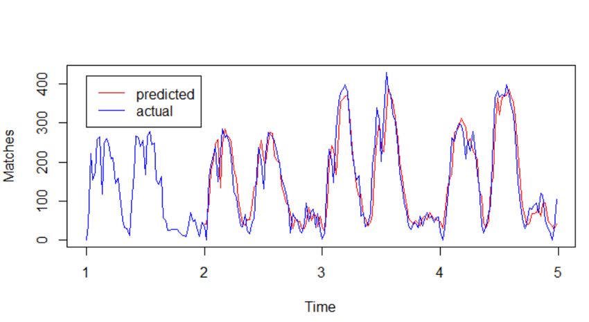
Table of Contents
1. Introduction 1
 1.1 Problematization 1
 1.2 Purpose 3
 1.3 Research Questions 3

2. Theory 4
 2.1 Seasonal Naïve Model 4
 2.2 Autoregressive Integrated Moving Average 4
 2.2.1 Seasonal ARIMA 5
 2.2.2 Box-Jenkins Methodology 6
 2.3 Neural Networks 7
 2.4 Evaluation measures 8
 2.4.1 Mean Error 8
 2.4.2 Root Mean Square Error 9
 2.4.3 Mean Absolute Error 10
 2.4.4 Mean Absolute Percentage Error 10
 2.4.5 Akaike Information Criterion 10

3. Data 11

4. Method 13
 4.1 Seasonal Naïve Model 13
 4.2 SARIMA 13
 4.3 Neural Network Autoregressive 15
 4.4 Model Evaluation 15

5. Results 16
 5.1 General Results 16
 5.2 LOL 17
 5.3 CS:GO 18
 5.4 Dota2 18
 5.5 Model Comparison 18

6. Analysis 19
 6.1 Seasonal Naïve Models 19
 6.2 SARIMA Models 19
 6.3 Neural Network Autoregressive Models 20

7. Conclusion 21

References 22

Appendix 24
 Appendix A 24
 Appendix B 25
 Appendix C 27
 Appendix D 29

1. Introduction
1.1 Problematization
In the beginning of the 80s the world was introduced to the first form of esports when
arcades, with a vast selection of games, opened all around the world. These electronic devices
would be the start of a whole new genre of sport, so called electronic sports (esports) (Lee
and Schoenstedt, 2011). Esport are, unlike traditional sports, a discussed form of sport
(Hamari and Sjöblom 2017; Jonasson and Thiborg 2010; Pizzo et al. 2018), where the actual
exercise happens through electronic environments or in “virtual worlds''. In practical terms,
esport is competitive gaming. Like traditional sports, the competition is between
human-human interactions, although in esport these interactions are facilitated by some
electronic media (Hamari and Sjöblom, 2017). This electronic media can be everything from
a gaming console to a personal computer (Pizzo et al. 2018). Furthermore, esport consist of a
broad spectrum of different games and genres, considered different (e)sports, and does not
necessarily have to mimic traditional sports even though some games do, like the soccer
game FIFA or the ice-hockey game NHL (Hamari and Sjöblom 2017; Pizzo et al. 2018).
Other games are closer to the perception of traditional gaming like the first-person shooter
Counter-Strike:Global Offensive (CS:GO) or the online battle arena games League of
Legends (LOL) and Defense of the Ancients 2 (Dota2) (Hamari and Sjöblom 2017). Based
on the definition of esport, there are simultaneous similarities and differences to traditional
sports.

Esport shares, in terms of structure, a lot of similarities with traditional sport with players
competing for different teams, players having managers and being subject for
player-transfers. Additionally, various esports have recently been introducing multiple
leagues and some colleges even offer esport scholarships (Pizzo et al. 2018). However,
differences are more present in terms of exercising the two; Firstly, the physical movements
required in esports are limited to small muscle groups with focus being on fine motor skills.
The second aspect that differs between the two is the availability of the sport. Esports can
only be exercised with access to the right equipment as well as under the supervision of

 1

institutions unlike most traditional sports where anyone can play without permission from
institutions or without access to expensive equipment (Jenny, et al. 2017). Whether or not
esport is to be considered a sport will not be further explored in this paper but rather
evaluated as a phenomenon.

Esport has seen an enormous growth in popularity and rising (Rosell Lloren, 2017). Among
the most popular under 2020 we find the games LOL, CS:GO and Dota2 chronologically,
exceeding a total of 1.1 billion hours watched (Borisov, 2021). As a result, the esport market
is expected to see a growth in size to about 32,5% by 2021 (Elasri-Ejjaberi,
Rodriguez-Rodriguez and Aparicio-Chueca, 2020) and to generate revenues near $2 billion
by the year of 2022 (Reyes, 2021). Considering the large revenues esport generates, many
large cap companies, such as Red Bull, Samsung, McDonald’s, Toyota and Microsoft, have
shown increased interest in the industry in terms of sponsors, thus exposing themselves to a
large new market (Elasri-Ejjaberi, Rodriguez-Rodriguez and Aparicio-Chueca 2020; Pizzo et
al. 2018). In extension, advertising and sponsorship stands for 69% of the cash flowing into
the esport industry (Reyes 2021). Not only large cap companies are drawn to the exploding
market that is esport but also private investors and venture capitalists (Newman et al., 2020).
While esport, as an industry, is growing rapidly the investments grow at an even quicker pace
(ibid). Meaning that the industry, as of now, attracts a variety of different stakeholders.

Reasonably, all the esport industry’s stakeholders have an interest in predicting the future of
the industry, thus securing their own interest on the market. In statistics, forecasting methods
are often used for predicting the future, especially when considering time series data. Several
different methods are available, the most proven method for forecasting is the ARIMA
model, following the Box-Jenkins methodology (Zhang, 2003). Even though this model has
shown satisfactory results, new methods for forecasting are constantly emerging. One such
method is forecasting using machine learning, or more specifically neural networks
(Makridakis, Spiliotis and Assimakopoulos, 2018). While these methods seem to be proven
on time series, there is to our knowledge, no forecasting research done on time series data
trying to predict the growth of esport as an industry nor the frequency of matches being
played. In addition to the fact that there is no relevant research done on this subject,

 2

comparing forecasting results can be challenging. A commonly used benchmark model is the
naïve model or the seasonal naïve model (Hyndman and Athanasopoulos, 2018; Makridakis,
Wheelwright and Hyndman, 1998).

1.2 Purpose
Ascending from the rapid growth in the esport industry, its many stakeholders and the fact
that no relevant academic research has applied forecasting methods on the growth of esport,
this paper aims to predict how many professional matches that will be played in the top three
most popular esports during the first three months of 2021. Furthermore, we aim to achieve
this by using proven forecasting methods and comparing them to a benchmark model.

1.3 Research Questions
Can we predict how many professional matches will be played during the first three months
of 2021 for the three most popular esports and if so, how accurately by using ARIMA and
neural networks models?

 3

2. Theory
In this section, three different statistical theories regarding forecasting will be explored;
seasonal naïve, autoregressive integrated moving average and neural networks in
chronological order. Lastly, error measures, that facilitate evaluation of these forecasting
methods, will be defined.

2.1 Seasonal Naïve Model
If you have belief that the value today will be equal to the value yesterday you might want to
consider using a Naïve model. Forecasting using this basic method will mean that the
predicted value will be equal to the last observed value (Hyndman and Athanasopoulos
2018).

Considering seasonal data, there is the Seasonal Naïve method which predicts each value as
equal to the same value last season. In this case predictions will be generated to be equal to
the last observed value 52 weeks earlier. The forecast for time T +h can be written as:

 , (5)

where m equals the seasonal period, and k is the number of years in the forecast period prior
to time T + h (Hyndman and Athanasopoulos 2018). Often a Naïve or Seasonal Naïve model
is used to compare other, more complex, models' error measures or accuracy (Makridakis,
Wheelwright and Hyndman, 1998).

2.2 Autoregressive Integrated Moving Average
In time series analysis the autoregressive integrated moving average model (ARIMA) is a
generalization of the autoregressive moving average (ARMA) model and is a common
forecasting method used in time series analysis. An ARIMA model can be interpreted as
three different parts with the first part referring to the autoregressive process. The
autoregressive process states that the output variable will depend linearly on its previous
values as well as an error term that represents what cannot be explained from the past values.

In order for this to be possible we have to assume that ( ) and that the error terms are
independent of the past values of yt all through the entire time series. An autoregressive

 4

process of order p, where B is the backshift operator, can be commonly expressed as an
AR(p) (Box, Jenkins and Reinsel 1994):

 . (1)

The MA part of the ARIMA model is referring to the moving average which does not use the
past values of the variable but instead relies on the past error terms to make forecasts of
future values. The present value can be found by adding weights to the previous error terms
(Box, Jenkins and Reinsel 1994). A moving average process of order q or a MA(q), can be
commonly expressed as (Cryer and Chan, 2008) :

 . (2)

Lasty we have an integration of the autoregressive process and moving average process of
some difference, d. The integration tells us that the data values have been replaced with the d
difference between their values and the d previous values. In usage of an ARMA model the
data needs to be stationary, meaning that the properties of the series should not depend on
time. One way of achieving this is by using an integrated ARMA (ARIMA) model. The
ARIMA model is in time series a common way to model non-stationary data where the d:th
difference, in general, generates a stationary ARMA process (Vandaele, 1983). We can
express a general ARIMA model as (Box, Jenkins and Reinsel, 1994):

 , (3)

where the term ϕp is the AR polynomial, θq is the MA polynomial and, again, B equals the
backshift operator with the d: th difference (Box, Jenkins and Reinsel 1994).

2.2.1 Seasonal ARIMA
A seasonal ARIMA (SARIMA) model is created by adding in seasonal components to the
ARIMA process. The seasonal components are similar to the non-seasonal components but
instead backshifts in regard to seasonal periods. The modelling procedure is very close to
ARIMA but we also need to choose seasonal AR(P) and MA(Q) terms for the model. The

 5

notation for a general SARIMA model can be expressed as SARIMA(p,d,q)(P,D,Q) with m

being the seasonal frequency. We can express a general SARIMA model as (Box, Jenkins and
Reinsel, 1994):

 , (4)

where is the seasonal autoregressive term, the seasonal moving average term and D
the seasonal difference.

2.2.2 Box-Jenkins Methodology
A popular and proven modelling process is the Box-Jenkins method, described by Box,
Jenkins and Reinsel (1994) and applied by many (e. g. Cryer and Chan, 2008; Makridakis and
Hibon, 1997; Makridakis, Wheelwright and Hyndman, 1998; Vandaele, 1983). It is an
iterative modelling process used in most practical situations when all information about the
object for forecasting is not available nor comprehensible (Box, Jenkins and Reinsel, 1994).
The process follows iterative steps to prepare data, identify and evaluate models and lastly
produce forecasts with the chosen model. Summarized, the methodology follows these steps
(Makridakis, Wheelwright and Hyndman, 2018):

 1. Data preparation
 2. Model selection
 3. Model estimation
 4. Model diagnostics
 5. Forecasting

The first step concerns the initial raw data. Here the data are evaluated and should be
transformed or differentiated in order to achieve a stationary time series. The second step
involves selecting a model based on examinations of the data’s autocorrelation function
(ACF) and partial autocorrelation function (PACF). Proceeding, to the third step, where
identified models are evaluated and selected based on established criterions. Fourthly, the
models are evaluated by diagnostics, e.g. testing residuals for autocorrelation. Only if the
models pass the fourth step, can they proceed to the last step of forecasting. If the model does
not pass the diagnostics, you must go back to step two where another model has to be

 6

specified that could pass the diagnostics in step four (Makridakis, Wheelwright and
Hyndman, 2018).

2.3 Neural Networks
Artificial Neural networks is a machine learning method that allows complex nonlinear
relationships between the response variable and its predictors. The method is based on the
human brain and how neurons are connected. Neural networks are commonly used for
classification purposes but have proven to be useful in other fields such as forecasting due to
their ability to capture non-linear relationships (Makridakis, Wheelwright and Hyndman,
1998).

Neural networks generally consist of three layers with connections from one layer to another
passing information along. Neural networks can feed information cyclical or in one direction,
a feed-forward neural network is passing along information in one direction (Hyndman and
Athanasopoulos, 2018). The first layer is called the input layer and consists of a number of
input values, these values enter nodes that later transfer the information onto the next layer.
Each node in the input layer is later connected to each node in the next layer creating a
complex network. The nodes are connected through the layers using weights , and and

these are obtained using a learning algorithm that minimises an error measure, like the Mean
Square Error (MSE). This means that the output of the nodes in one layer are then inputs in
the next. The intermediate layer is called the hidden layer. Like the input layer; the hidden
layer contains nodes and is what makes the neural network non-linear. A neural network with
no hidden layer is equivalent to a normal linear regression (Hyndman and Athanasopoulos,
2018).

The inputs to each node in the hidden layer are combined using a weighted linear
combination which is later modified by a nonlinear function before being treated as output.
The input to each j node in the hidden layer is calculated as

 (6)
 ,

where n is the number of nodes in the input layer and j is the amount of nodes in the hidden
layer. In the hidden layer, the output is modified before being input to the next layer using a

 7

nonlinear function such as the sigmoid function. The general formula for the sigmoid
function:

 (7)
 .

The sigmoid function tends to reduce the effect of extreme values and thus making the
method somewhat suitable for data containing outliers. The modified values become input
values to the next layer which could either be more hidden layers or a final output layer.

To train the neural network, the weight starts off by taking on random values which are later
updated using the observed data. By doing so there is an element of randomness in the neural
network’s predictions. Therefore, a normal approach is to train the network several times
using random starting points and then taking the average of the results. The model is later
tested against new data to give an idea of its accuracy (Hyndman and Athanasopoulos, 2018).

Using neural networks with time series data, the lagged values of the time series can be used
as input values in the first layer. This is called a neural network autoregressive (NNAR)
model. The model has similarities to an AR model but uses the structure of a neural network.
The NNAR, similar to the SARIMA model, performs multi-step forecasting by taking
predicted values into account for further predictions (Hyndman and Athanasopoulos, 2018).
For this report, we use the notation NNAR(p,P,k)m where p is the number of lagged inputs, P
is the amount of last observed values from the same season, k is the number of nodes in the
hidden layer and m is equal to the seasonal frequence. The NNAR model does not require the
data to be stationary in order to train the model, however transforming the data can
sometimes help to improve the model accuracy (Hyndman and Athanasopoulos, 2018).

2.4 Evaluation measures

2.4.1 Mean Error
The mean error (ME) is one of the most basic error measures. It is simply calculated by
dividing the sum of the actual values minus the predicted values by the number of
predictions. Although using the ME as an evaluation measure can be misleading since
negative and positive errors can cancel each other out and thus displaying a good model when
it is in fact not (Hyndman and Athanasopoulos 2018). In this study the ME is used as a quick

 8

overview for under- or overestimation in the predictions rather than a tool for forecasting
accuracy. The formula for ME:

 (8)
 ,

where is the actual value and is the predicted value.

2.4.2 Root Mean Square Error
The root mean square error (RMSE) takes the root of the MSE. Meaning that the measure
takes the square root of the squared difference between the predicted values and the actual
values. The value of the RMSE is hard to interpret by itself but can be a useful tool when
comparing multiple models, applied on the same data set (Hyndman and Athanasopoulos
2018). RMSE is calculated as by:

 (9)
 .

 9

2.4.3 Mean Absolute Error
The mean absolute error (MAE) is similar to the ME but measures the errors in absolute
values. This calculation will then provide a strictly positive output where negative or positive
error does not cancel each other out, like the case with ME. Meaning, that the MAE gives a
more accurate measure on how well the model fits the data given that all the absolute errors
summarize (Hyndman and Athanasopoulos 2018). The formula for MAE is:

 (10)
 .

2.4.4 Mean Absolute Percentage Error
The mean absolute percentage error (MAPE) is an error measure that can be used to compare
models between different data sets given that it does not take the measuring unit into account
but rather outputs the errors in percentage. The calculations are computed by:

 (11)
 ,

where ei is derived as earlier. This lets us calculate the percentage error for a given time point
(Hyndman and Athanasopoulos, 2018).

2.4.5 Akaike Information Criterion
The Akaike information criterion (AIC) is a method used for model selection (Akaike, 1974).
The main objective of the AIC is to estimate the relative loss of information for different
models. The criterion is designed in a way that makes it easy to compare models by choosing
the model with the lowest AIC value. The AIC is defined as:

 (12)

where the term k takes the number of parameters in the model into consideration. When using
an ARIMA model the term equals to k = p + q + 1 with the constant 1 referring to if an
intercept is included in the model. If there is no intercept in the model the constant 1 is
removed. The purpose of the term k is to penalize the model for overfitting (Akaike, 1974).

 10

3. Data
In this section the data used for the study will be presented as well as any transformations
made to it.

The data used in this study have been acquired through Abios Gaming which are a world
leading data supplier within the esport industry. Abios have since 2015 been collecting high
quality data on a broad selection of esport genres using various data collection methods
(Abios, 2021). How Abios defines a “professional esport match” is according to Franscensco
Katsoulakis1 “In general, we collect data on all esports matches for the first three divisions in
each respective game”, which describes how our data are collected. So, only matches played
in the top three divisions of respective games will be used.

The three games used in the study are all played on a global level, meaning that the data
covers many different time zones. With this in mind, we could assume that specific regional
deviations, e.g. holidays, that could affect the amount of matches are not indicative enough to
be taken into account when building the models.

The time series data used in this report spans from January 2017 to and including March
2021. The first four years, i.e. 2017 through 2020, is used to create the models and the first 12
weeks in 2021 is used to evaluate them. The data, that are collected on an hourly basis, have
been aggregated to a weekly basis as hourly predictions would, not exclusively, be difficult to
conduct but also irrelevant for stakeholders. The time period corresponds to 221 weeks with a
total of 142 381 covered matches in the three games LOL, CS:GO and Dota2. All years had
52 weeks except the year of 2020 which had 53 weeks. Given this, the week 52 and 53 in
2020 have been merged together to fit a 52 weeks year schedule. This has been done in order
for our seasonal models to operate accurately with the seasonal difference taken into account,
since it could severely harm the predictions otherwise (Hyndman and Athanasopoulos 2018).
In addition, this data manipulation did not render any extreme values, which indicates that
there is no meaningful harm done to the data.

The time it takes for one match to be played varies within the different games. The game
setting in LOL and Dota2 are similar, although the average game length in professional play

1
 Franscensco Katsoulakis, Head of Data Quality, Abios Gaming AB, verbally, 10th of May 2021.

 11

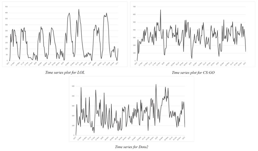
varies with Dota2 averaging 45 minutes (Hassall, 2020) and LOL matches lasting on average
for 32 minutes (Games of Legends Esport, 2021). Professional CS:GO matches have been
known to take 45 minutes on average (Scales, 2020).

 Figure 3.1. Overview of Figures B.1, B.2 and B.3.

In Figure 3.1, overviewing Figures B.1, B.2 and B.3 in Appendix, we can observe the amount
of matches played every week for the three different games. We can see that the game with
the most played professional matches is CS:GO with yearly peaks at around 500 matches.
Dota2 peaks higher than LOL during some weeks but the LOL matches display a more
seasonal pattern. A reason for this might be that Riot Games, the creator of LOL, operates all
professional leagues and tournaments in the game (Rosell Llorens, 2017). The matches in
Dota2 do not seem as dependent on seasons, although we can see that during some weeks a
large amount of matches are being played.

 12

4. Method
In this section each of the chosen theories' respective methodology will be described in detail.

4.1 Seasonal Naïve Model
By ocularly inspecting the time series plots (see Figure 3.1), some seasonality seems present.
Hence, we choose to apply a seasonal naïve model as our benchmark. The model is applied to
each data set respectively using the snaive() function from the forecast package in R,
predicting that the value of the first week in January 2021 will use the same value as for the
first week in January 2020 and so forth. The models are evaluated using the error measures
defined in Section 2.4.

4.2 SARIMA
The method workflow applied when modelling the (S)ARIMA models is the Box-Jenkins
methodology. Hence, we will follow the steps of the iterative steps defined in Section 2.2.2.

Now when we initially have seen the data, we will proceed to work with it to formulate
models in order to perform forecasts of the first twelve weeks of 2021. In order for SARIMA
modelling to make sense at all, the data needs to contain at least some correlation. By looking
at correlograms we can identify that all data sets contain enough correlation to continue with
our modelling and carry out analysis.

As an initial step, an ocular inspection of the time series plots in Figure 3.1 is done where it is
hard to identify any clear trends in either of the data sets. Hence, we perform the Augmented
Dickey-Fuller (ADF) test to check the three data sets for a unit root. The hypothesis is written
as:

The data for LOL and CS:GO makes us reject the null hypothesis, meaning that on the five
percent significance level there is no unit root. Thus these two data sets are stationary and are
ready to proceed in the modelling process. However, the test on the data for Dota2 did not
make us reject the null hypothesis, suggesting a unit root is present meaning the data are not

 13

stationary. So, this data set needs transformation, or detrending, in order to proceed in the
modelling process. To detrend the data, the first difference is used which should make the
data stationary. However, to be sure the first difference did successfully detrend the data set,
the ADF test is repeated. Now we can reject the null hypothesis on the five percent
significance level and state that this time series is stationary and thus fulfills the requirements
to proceed in the modelling process. Now all data sets show correlation and stationary. Hence
they can proceed to the model selection step. For test output, see Table A.1 in Appendix.

For model selection the correlation of the data is used for modelling by reviewing its ACF
and PACF in order to choose a model. We perform an ocular inspection of the ACF and
PACF for the respective data sets to identify a (S)ARIMA model that could be a good fit for
the data. While this method does not necessarily suggest that the chosen model is the “best”
fit (Makridakis, Wheelwright and Hybdman, 1998), it does however give some indication.
For LOL and CS:GO we identify that an ARIMA(1,0,0) model seems to be a good fit and we
then test different models with varying seasonal components for both data sets. While
inspecting the ACF and PACF for the differentiated data for Dota2, it is not as clear as for the
other data sets. Different SARIMA models are chosen for testing, mainly ARIMA(1,1,1) and
ARIMA (2,1,1), both with various seasonal components. Proceeding with the estimation and
model evaluation diagnostics.

Mainly the error measures ME, RMSE, MAE and AIC are used for model evaluation. All
these measures indicate, in varying manners, how large the error is for each model,
consequently how far the predictions are from the actual values. Point being that low values
on the error measures indicates that the model lies closer to the actual values in its prediction.
Firstly, we look at the in-sample-errors for these measures, which gives an indication on how
the model will perform when trying forecasting. So, the models with the lowest errors over
the different measures will be chosen for forecasting. However, we can see that different
models possess lowest values on different measures, see Table 5.1. Hence, all models will
proceed to the forecasting step in order to evaluate which model renders the most accurate
predictions.

However, before the models will be used for forecasting, respective model’s residuals need to
be tested for autocorrelation. This is done by the Ljung-Box test in order to identify if the

 14

residuals are random and hence indicating that the model is an adequate fit given data. The
test is performed with 20 lags and the hypotheses for the test are:

For test output see Table 5.1 in the Result section.

Lastly, the models that pass step four can proceed to forecasting. The in- and out-of-sample
errors are reviewed and compared to each game’s respective seasonal naïve model to evaluate
which model produces the most accurate predictions. Also the out-of-sample MAPE for each
model is reviewed based on the interpretability and simultaneously enabling us to compare
models between data sets.

4.3 Neural Network Autoregressive
The function nnetar() in R, created by Hyndman and Athanasopoulos (2018), has been used
to estimate the models’ parameters. The NNAR model for Dota2 has been constructed on the
first difference dataset in order to achieve higher accuracy. The function uses MSE as an error
measure and decides the optimal number of lags, p, according to the AIC for a linear AR(p)
model fitted to the seasonal data. Where k is calculated by k = (p + P + 1)/2 if not specified
beforehand. In this study the NNAR models have been constructed using 20 networks fitted
with random starting weights. These are later averaged when producing forecasts for the first
twelve weeks in 2021. The point forecasts are compared to the actual data to calculate the
out-of-sample evaluation error measures. Lastly, the out-of-sample, used earlier, will be used
to compare the rendered models individually and in comparison to the seasonal naïve
benchmark model.

4.4 Model Evaluation
The different models have been evaluated using the aforementioned evaluation measures in
Section 2.4. A specific model is considered to be superior if the majority of the evaluation
measures are more accurate than another model.

 15

5. Results
In this section the results will be displayed and further defined. Structure wise, general
results are presented followed by results from LOL, CS:GO and Dota2 as well as a model
comparison.

5.1 General Results
As mentioned in Method, all data sets were tested for stationarity with the Dickey-Fuller test,
see Table 9.1 in appendix for test output. LOL and CS:GO showed no sign of a unit root
being present on the five percent significance level, hence to be considered stationary.
However, when performing the test on Dota2 we could not reject the null hypothesis on the
five percent significance level. Thus, the data were transformed into first difference and
tested again. After the data manipulation we were able to reject the null hypothesis and thus
consider the data to be stationary. Given that all data sets are stationary they could all proceed
into the modelling process, which are presented next in this section.

In Table 5.1 the results from the model testing are presented. Similarities in the LOL and
CS:GO dataset resulted in the same models being applied to both datasets. Models for each
game are displayed, together with their respective in- and out-of-sample error measures and
also their produced Ljung-Box test p-value. Worth noting is that the models for Dota2 differ,
given the nature of the data, from the models for LOL and CS:GO. The lowest value
produced for each game’s evaluation measures is bold. Also, the model with the lowest
values produced overall for in- and out-of-sample are marked with blue and green
respectively.

 16

Table 5.1: results from model evaluation, forecasting and Ljung-Box test.

From Table 5.1 we can see p-values generated from the Ljung-Box tests, where we can
identify that many of the different models’ residuals show no sign of autocorrelation on the
five percent significance level, except all the naïve models and SARIMA(1,0,0)(0,1,0)52 when
applied on the data for CS:GO.

Furthermore, we can see that most in-sample evaluation measures in our models are lower
than the out-of-sample measures. These measures provide an indication for which model fits
the data well. However, to ultimately evaluate the models, the out-of-sample counterpart is
considered to see how well the models performed when exposed to new data.

5.2 LOL
By firstly inspecting the in-sample measures for the models applied on LOL we can see that
the SARIMA(1,0,0)(0,1,1)52 generates the lowest values for all measures except for the
NNAR(1, 1, 2)52 that generates the lowest ME. However, when observing the out-of-sample

measures we can see that the SARIMA(1,0,0)(1,1,1)52 outperforms all the other models, even
though it performs with lesser accuracy than it did in-sample.

 17

5.3 CS:GO
When observing the model outputs for CS:GO we can see, again, that the SARIMA
(1,0,0)(1,1,1)52 model outperforms the other models, in-sample, over all measures except the
NNAR(1, 1, 2)52 which achieves lower ME. Proceeding with the out-of-sample measures we

can observe that the NNAR outperforms the other models except the SARIMA(1,0,0)(1,0,0)52
which has a lower ME.

5.4 Dota2
Lastly, we consider the results for Dota2. Again, the models used for predicting Dota2 differs
from the models used for the other games. Evidently we can see that the NNAR(9, 1, 6)52

model, which also differs in structure from the NNAR:s for the other esports, outperformed
the other models based on the in-sample measures, except for the AIC that is not produced
for the NNAR where the lowest value were obtained by the SARIMA(1,1,1)(0,1,1)52.
However, the NNAR performs worse in the out-of-sample measures. The lowest
out-of-sample error measures for RMSE and MAE were given by a SARIMA(1,1,1)(0,0,1)52
and the lowest ME were produced by a SARIMA(2,1,1)(0,1,0)52 model.

5.5 Model Comparison
In Table 5.2 we summarize the models with the lowest out-of-sample values for each game
using the evaluation measure MAPE. Firstly, the highest MAPE is achieved by the SARIMA
model for LOL with a value of 77%. Secondly, the SARIMA model for the Dota2 data
produces a MAPE of approximately 41%. Lastly, the NNAR model fitted to the CS:GO
dataset generates the lowest MAPE of roughly 31%.

 Table 5.2: results from model evaluation based on MAPE.

 18

6. Analysis
In this section an analysis of the results is conducted with regard to our chosen methods.
Each method is analysed in chronological order.

6.1 Seasonal Naïve Models
Looking at our results we can see that our most simple model, the seasonal naïve model,
performed badly in comparison to the other models. The seasonal naïve model, for all three
games, showed either large under- or overestimations except for in-sample for CS:GO, based
on the ME values. All the Ljung-Box tests for the seasonal naïve models were significant,
which is a general warning sign for a bad prediction model (Hyndman and Athanasopoulos
2018). Even though this is not applicable for a naïve model, given that the model only uses
the last observed values for predictions, it can still indicate a bad prediction model. To
illustrate, the out-of-sample ME for Dota2 were substantially larger than for the other models
for Dota2 as well as negative, meaning that the seasonal naïve model for Dota2
over-estimated the amount of matches for the prediction period but underestimated for the
training period. The results for the seasonal naïve models indicate that the seasonality in the
datasets vary over the years and that other tools might be necessary in order to capture the
variation. The reason for this might be the usage of the weekly calendar, in which one
specific year's weeks would not correspond to the same dates the next coming year.

6.2 SARIMA Models
For the SARIMA models in LOL and CS:GO we could see that the SARIMA(1,0,0)(0,1,1)52
and SARIMA(1,0,0)(1,1,1)52 produced very similar results and that in both games the model
with a seasonal AR-term performed better for the test period than the training period. The
differences in evaluation measures between the two models are small in both games which
raises the question whether they are significantly different from each other.

The models, fitted to the LOL dataset, display relatively large differences between in- and
out-of-sample measures in comparison to CS:GO and Dota2. We can see that the smallest
differences between in-sample and out-of-sample values are in the CS:GO models. For both
LOL and CS:GO we can identify, for all models, positive and quite large mean errors. For
Dota2 the opposite is true with almost all models showing negative mean errors as well as
relatively small ones. Furthermore, some of the SARIMA models for Dota2 displayed

 19

out-of-sample values to be lower than those in-sample. To elaborate, predicting the amount of
matches has proven itself to be difficult, where the in-sample evaluation measures clearly not
being a guarantee for accurate forecasts. This is also supported by the fact that all the models,
in all the games, with lowest in-sample values were not the most accurate when applied to
new data.

6.3 Neural Network Autoregressive Models
In overall the Neural networks performed well on the training data, especially for the Dota2
dataset where it is substantially better than the other models. Although, the NNAR models
have difficulties on the test data except for the CS:GO data where it outperformed all the
other models. Looking at Figure B.1, B.2 and B.3 in Appendix, we can see the NNAR models
fitted to the training dataset. Following the graphs, The NNAR models for LOL and Dota2
appear to be overfitting but the NNAR model for CS:GO appears not to. The evaluation
measures in Table 5.1 also confirms this with the small differences between in- and
out-of-sample values for the NNAR model in CS:GO. The reason for this can be explained by
the operational process where the NNAR model decides the optimal number of lags p
according to the AIC for a linear AR(p) model fitted to the seasonal data. This process
resulted in a NNAR(1, 1, 2)52model for CS:GO which could not capture all the variation in

the data.

 20

7. Conclusion
So, are we able to predict how many matches will be played in these three esports during the
first three months of 2021 and if so, how well?

In conclusion, the data allowed time series modeling and analysis. Meaning, we were able to
predict, with statistical insurance, how many matches that would be played in the first three
months of 2021 for the three esports, LOL, CS:GO and Dota2. In terms of how accurate these
predictions are, they were able to outperform the benchmark seasonal naïve models. Overall,
the most accurate model is the NNAR model for CS:GO, which achieved a MAPE of roughly
31%, in comparison to the most accurate model for LOL and Dota2 which achieved a MAPE
of 77% respectively 41%. However, the answer to how accurate our models are is arbitrary
and solely depends on how far the predicted values are allowed to be from the actual values.

 21

References
Abios Gaming AB. (2021). About. https://abiosgaming.com/about/ [retrieved 2021-05-15]

Akaike, H. (1974). A new look at the statistical model identification. IEEE transactions on
automatic control. 19(6): 716-723.

Borisov, A. (2021). Most popular esports games in 2020.
https://escharts.com/blog/most-popular-esports-games-2020 [retrieved 2021-05-19].

Box, G.E.P., Jenkins, G.M. & Reinsel, G.C. (1994). Time series analysis: forecasting and
control. 3rd ed. New Jersey: Prentice Hall.

Cryer, J.D. & Chan, K. (2008). Time series analysis: with applications in R. 2nd ed. New
York: Springer.

Elasri-Ejjaberi, A., Rodriguez-Rodriguez, S. & Aparicio-Chueca, P. (2020). Effect of eSport
sponsorship on brands: an empirical study applied to youth. Journal of Physical Education
and Sport. 20(2): 852-861

Games of Legends Esport. (2021). World Championship 2020: Overview.
https://gol.gg/tournament/tournament-stats/World%20Championship%202020/ [retrieved
2021-05-24]

Hamari, J. & Sjöblom, M. (2017). What is eSports and why do people watch it. Internet
research. 27(2): 211-232.

Hassall, M. (2020). The Longest Games in Dota2 History.
https://www.hotspawn.com/dota2/guides/the-longest-games-in-dota-2-history [retrieved
2021-05-24]

Hyndman, R.J., & Athanasopoulos, G. (2018) Forecasting: principles and practice, 2nd ed.
Melbourne: OTexts. OTexts.com/fpp2 [retrieved 2021-05-18]

Jenny, S.E., Manning, R.D., Keiper, M.C. & Olrich, T.W. (2017). "Virtual(ly) Athletes:
Where eSports Fit Within the Definition of "Sport". Quest (National Association for
Kinesiology in Higher Education). 69(1): 1-18.

Jonasson, K., Thiborg, J. (2010). Electronic sport and its impact on future sport. Sport in
society. 13(2): 287-299.

 22

Katsoulakis, F. (2021-05-10). Head of Data Quality. Abios Gaming AB. Verbally.

Lee, D. & Schoenstedt, L.J. (2011). Comparison of eSports and Traditional Sports
Consumption Motives. The ICHPER-SD Journal of Research in Health, Physical Education,
Recreation, Sport & Dance. 6(2): 39-44.

Makridakis, S. & Hibon, M. (1997). ARMA Models and the Box–Jenkins Methodology.
Journal of forecasting. 16(3): 147-163.

Makridakis, S., Spiliotis, E. & Assimakopoulos, V. (2018). Statistical and Machine Learning
forecasting methods: Concerns and ways forward. PloS one. 13(3): e0194889-e0194889.

Makridakis, S.G., Wheelwright, S.C. & Hyndman, R.J. (1998). Forecasting: methods and
applications. 3rd ed. New York: John Wiley & Sons.

Newman, J.I., Xue, H., Watanabe, N.M., Yan, G. & McLeod, C.M. (2020). Gaming Gone
Viral: An Analysis of the Emerging Esports Narrative Economy. Communication and sport.

Pizzo, A.D., Baker, B.J., Na, S., Lee, M.A., Kim, D. & Funk, D.C. (2018). eSport vs. Sport:
A Comparison of Spectator Motives. Sport marketing quarterly. 27(2): 108-123.

Reyes, M. S. (2021). The key industry players and trends growing the esports market which
is on track to surpass $1.5B by 2023. Business Insider.
https://www.businessinsider.com/esports-ecosystem-market-report [retrieved 2021-05-19]

Rosell Llorens, M. (2017). eSport Gaming: The Rise of a New Sports Practice. Sport, ethics
and philosophy. 11(4): 464-476.

Scales, K. (2020). A Beginner’s Guide To Esports: Counter-Strike: Global Offensive.
https://checkpointxp.com/2020/04/17/a-beginners-guide-to-esports-counter-strike-global-offe
nsive/ [retrieved 2021-05-24]

Vandaele, W. (1983). Applied time series and Box-Jenkins model. San Diego: Academic
Press.

Zhang, G.P. (2003). Time series forecasting using a hybrid ARIMA and neural network
model. Neurocomputing (Amsterdam). 50: 159-175.

 23

Appendix

Appendix A
 Table A.1: ADF test output for all games with p-values

 24

Appendix B

 Figure B.1: Time series plot for LOL

 Figure B.2: Time series plot for CS:GO

 25

Figure B.3: Time series for Dota2

 26

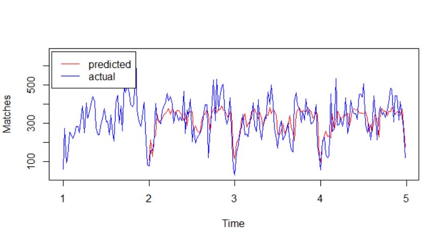
Appendix C

 Figure C.1: NNAR model over time series plot for LOL

 Figure C.2: NNAR model over time series plot for CS:GO

 27

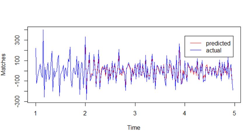
Figure C.3: NNAR model over first differenced time series plot for Dota2

 28

Appendix D

 Figure D.1 : predicted value over actual value for LOL SARIMA (1, 0, 0)(0, 1, 1) 52

 Figure D.2: predicted value over actual value for CS:GO NNAR (1, 1, 2)52

 29

Figure D.3: predicted value over actual values for Dota2: SARIMA (1, 1, 1)(0, 0, 1)52

 30