SEMANTIC SEGMENTATION OF BENTHIC COMMUNITIES FROM ORTHO-MOSAIC MAPS
←
→
Page content transcription
If your browser does not render page correctly, please read the page content below
The International Archives of the Photogrammetry, Remote Sensing and Spatial Information Sciences, Volume XLII-2/W10, 2019
    Underwater 3D Recording and Modelling “A Tool for Modern Applications and CH Recording”, 2–3 May 2019, Limassol, Cyprus

 SEMANTIC SEGMENTATION OF BENTHIC COMMUNITIES FROM ORTHO-MOSAIC
                              MAPS

                                     G. Pavoni1,2∗, M. Corsini2,3 , M. Callieri 2 , M. Palma 4 , R. Scopigno 2

                            1
                           Dipartimento di Ingegneria dell’Informazione, Università degli Studi di Pisa, Italy
                           2
                             Istituto di Scienze e Tecnologie dell’Informazione ”A.Faedo”, CNR, Pisa, Italy
                    3
                      Dipartimento di Ingegneria ”Enzo Ferrari”, Università degli Studi di Modena e Reggio Emilia
               4
                 Dipartimento di Scienze della Vita e dell’Ambiente, Università Politecnica delle Marche, Ancona, Italy

                                                           Commission II, WG II/9

KEY WORDS: Underwater Monitoring, Ortho-mosaic Map, Semantic Segmentation, Coral Reefs

ABSTRACT:

Visual sampling techniques represent a valuable resource for a rapid, non-invasive data acquisition for underwater monitoring purposes.
Long-term monitoring projects usually requires the collection of large quantities of data, and the visual analysis of a human expert
operator remains, in this context, a very time consuming task. It has been estimated that only the 1-2% of the acquired images are later
analyzed by scientists (Beijbom et al., 2012). Strategies for the automatic recognition of benthic communities are required to effectively
exploit all the information contained in visual data. Supervised learning methods, the most promising classification techniques in this
field, are commonly affected by two recurring issues: the wide diversity of marine organism, and the small amount of labeled data.
In this work, we discuss the advantages offered by the use of annotated high resolution ortho-mosaics of seabed to classify and segment
the investigated specimens, and we suggest several strategies to obtain a considerable per-pixel classification performance although the
use of a reduced training dataset composed by a single ortho-mosaic. The proposed methodology can be applied to a large number of
different species, making the procedure of marine organism identification an highly adaptable task.

                       1. INTRODUCTION                                     In section 2 we describe the advantages of working on polygon-
                                                                           annotated ortho-photo map when training CNN architectures. Then,
                                                                           we discuss several simple strategies, exploiting the properties of
In recent years, neural networks have been successfully used to
                                                                           the starting data, to improve the per-pixel classification perfor-
recognize marine organisms. In particular, CNN have demon-
                                                                           mance.
strated to obtain reasonably good performance in the segmen-
tation of benthic communities (King et al., 2018, Alonso et al.,
2017). While speeding up the recognition step, the use of neu-                • A biologically-inspired method to partition the input map
ral networks require the preparation of a large training dataset.               into the training, validation and test datasets.
The commonly used labeling methodology for underwater clas-
                                                                              • A simple but effective oversampling method, able to cope
sification is a point-based manual annotation on all the photos
                                                                                with the class imbalance problem.
of the input dataset, that has to be carried out by experienced
personnel, resulting in a very time-consuming process. To our                 • A way to aggregate network scores using the prior infor-
knowledge, when using point-wise annotations, all the existing                  mation about the actual coverage of the specimens on the
approaches based on SVM, CNN or FCNN models ((Beijbom et                        surveyed area.
al., 2015), (King et al., 2018), (Alonso et al., 2017), (Mahmood
et al., 2016)) adopt a patch-based labeling, cropping a square area        Finally, as a final step in our workflow, we employ a validation
around each annotated point. The Patch-based labeling could                tool, to analyze the semantic segmentation of complex natural
lead to sparse training datasets (Alonso et al., 2017); further-           structures (Pavoni et al., 2019). This tool can be used to val-
more, the annotated points falling close to the contours of the            idate the network predictions, or to correct the human labeling
specimen introduce a certain amount of uncertainty in the anno-            inconsistency, feeding back into the network a cleaner and en-
tation, depending on the size of the extracted patch. In (King             hanced dataset for a possible re-training step. The improvements
et al., 2018) the authors compare the performance of the state             obtained by introducing these methods in the network training
of the art architectures, using different annotation types. Best           and execution are outlined in section 4.
results were obtained by free-hand drawing labels on the inves-
tigated specimens, however, producing a similar dataset is ex-
tremely time-consuming. Nowadays, the polygonal annotation of                                        2. METHODS
ortho-mosaics inside GIS tools is a raising trend among biologists
that employ geo-referenced maps to study the spatial distribution          Coral reefs are populated by a huge amount of species, and since
of populations. In this work, we analyze efficient ways to use this        we are working with RGB images, learning to classify them co-
new, available, data format for the training of a semantic segmen-         incide with learning some peculiar features in their morphology
tation CNN for benthic communities.                                        and color. However, the task of identifying this features by pho-
                                                                           tographs, both for human users and for supervised learning meth-
  ∗ Corresponding   author (gaia.pavoni@isti.cnr.it)                       ods, is complicated not only by the intraspecific mutability of

                                                  This contribution has been peer-reviewed.
                     https://doi.org/10.5194/isprs-archives-XLII-2-W10-151-2019 | © Authors 2019. CC BY 4.0 License.                    151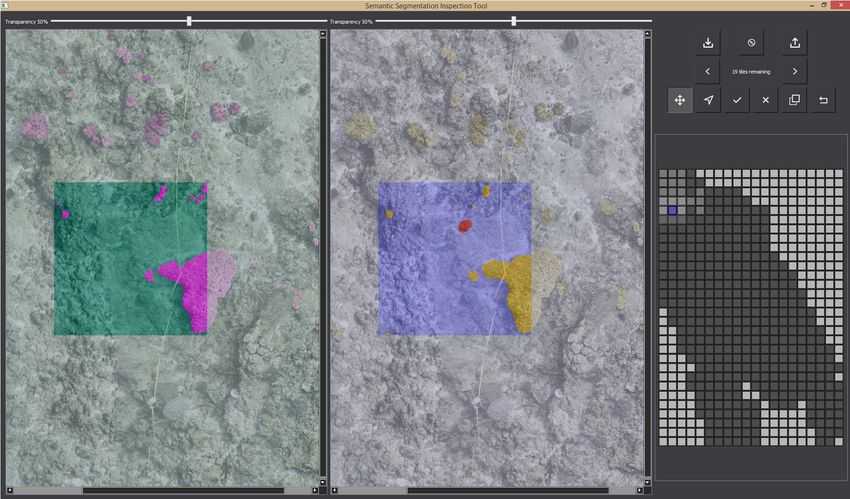
The International Archives of the Photogrammetry, Remote Sensing and Spatial Information Sciences, Volume XLII-2/W10, 2019
Underwater 3D Recording and Modelling “A Tool for Modern Applications and CH Recording”, 2–3 May 2019, Limassol, Cyprus
marine organisms, but also by environmental factors, by perspec-
tive issues or by the flaws of underwater images. The same coral
colony, framed from a different view angle or distance may ap-
pear totally different. Underwater photos are affected by color
and sharpness changes (due, respectively, to the water absorp-
tion of some wavelenghts and to the turbidity), by distortions and
by chromatic aberrations (caused by the interaction of the cam-
era lens with the port of the camera housing and with the water
medium). From a machine learning perspective, the use of ortho-
mosaic maps reduce the amount of factors to learn by removing
some of the described inconsistencies.
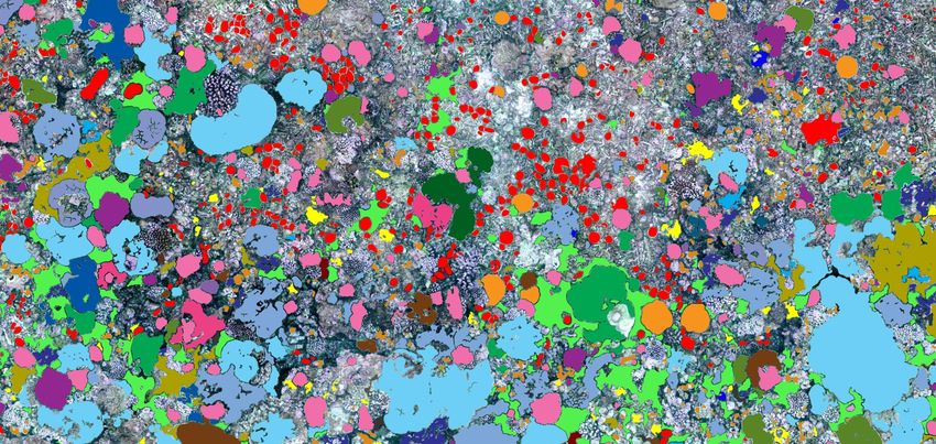
Figure 1. Coral class distribution. Courtesy of Scripps
Ortho-mosaics maps are rectified, have a constant pixel size, and Institution of Oceanography.
always present an azimuthal viewpoint, framing all the speci-
mens with a coherent view direction. Additionally, color vari- intrinsically uniform, such as the ones for the automatic recogni-
ations across photos are smoothed out by the blending process, tion of pedestrian and cars. However, in our case, we are dealing
and chromatic aberration is mostly removed. These factors re- with a continuous space (the reef map), where the organisms fol-
duce the non-biological variability of the corals images, help- low a non-uniform population distribution (Edwards et al., 2017).
ing the network to learn what really differentiates them from a For these reasons, instead of subdividing the data into random
biological-only perspective. non-overlapping parts, we chose three sub-areas of the monitored
Ortho-mosaics incorporate information of the actual metric scale, seabed by using ecology metrics describing the spatial patterns of
depth and the geographical coordinates. The output of the net- benthic communities.
works can be easily used for computing specimen areas, abun- Among all the landscape ecology metric commonly used (and im-
dance and coverage of the species. From the perspective of the plemented in many popular software such as FRAGSTAT) we se-
coral segmentation task, the physical size of morphological fea- lect three that describe the colonies distribution and are invariant
tures, as well as the depth of the coral colonies, are a discriminant to the shuffle of the tiles. The Patch Size Coefficient of Variation:
factor in classification.
Thanks to geo-referencing, identified objects can be relocated in 100.0 · std(Coral’s areas on the Patch)
P SCV = ,
a three dimensional context preserving the spatial distribution of mean(Coral’s areas on the Landscape)
the specimen as an additional and valuable information support-
ing monitoring activity. which measures the standard deviation of the size of specimens as
As we will show in the next, working with maps also allows us to a percentage of the mean size all over the dataset. It is commonly
exploit the scale and the spatial distribution of the population to used to describe the landscape area variability. Patch Richness
solve issues commonly found in preparing training datasets, such and Patch Coverage are related, respectively, to the number and
as the partition and the class imbalance. density of specimens. Obviously, other metrics can be integrated
Finally, inspired by the polygonal annotation made by (Palma in this method: for example, at the moment we are not consider-
et al., 2017) for the calculation of biometric indicators, we used ing metrics related to the perimeters because our polygon labeling
the manual polygonal labeling as an annotation solution for a is not that much detailed.
supervised learning dataset. In this context, with respect to the
point-wise photographic annotation, the use of ortho-photo mo- The selection criteria proceeds by choosing on the map a couple
saic seabed maps leads to faster labeling time, since drawing an of non overlapping windows (our Patches) of the approximately
approximate polygon around a specimen is faster than annotate dimensions of about the 15% of the entire surveyed area. Met-
hundreds of points on several images. Additionally, the polygo- rics are computed on each window and on the remaining area; a
nal annotation allows the use of a segmentation network instead weighted sum of the calculated values is assigned to each of the
of a patch-based classification one, providing a pixel-wise classi- three regions as a similarity score (S). This process is iterated an
fication. arbitrary number of times (∼ 10, 000), and then the triplet with
the best values of S is chosen as validation, test and training area
While solving many issues, ortho-photo mosaics may introduce respectively.
different problems. Small registration errors of the input images In order to combine the metrics in a weighted sum in an homo-
may cause local blurring or ghosting in the final map, that have geneous way, we express them in percentage w.r.t the statistics
to be somehow recognized and removed from the input dataset. of the labeled population. The weight used have been set em-
The stitching and projection process causes local image warping pirically after some tests. Values of S close to 0.0 means that
close to geometric discontinuities (e.g. the borders of the more the three areas have very similar statistical characteristics, great
protruding corals), we overcome this problems by masking these values that the area chosen are very different w.r.t the population.
areas to exclude them from the loss computation.
This strategy is trivial when applied on a single class, but still pro-
2.1 Biologically-inspired dataset partition duces a better balanced partition with respect to a random choice.
When the number of classes to segment increases, this method
Typically, to train a network in a reliable way, the available input will give an even stronger advantage, as a manual selection would
data is split into three datasets: one for the actual training, one for be impractical and a random process would not be viable.
the validation (used to tune the network’s hyper-parameters) and The image on the figure 1 is a labeled ortho-projection of a three-
one for the testing of the network performance (to assess the gen- dimensional reef reconstruction carried out by the Scripps Insti-
eralization capability of the trained network). In order to properly tution of Oceanography (100 Islands Challenge Team, 2019); this
work, these three datasets must be representative of the whole clearly shows how difficult it might be to manually select areas
data. A simple random partition works well in datasets which are displaying an adequate class representation. For such complex
This contribution has been peer-reviewed.
https://doi.org/10.5194/isprs-archives-XLII-2-W10-151-2019 | © Authors 2019. CC BY 4.0 License. 152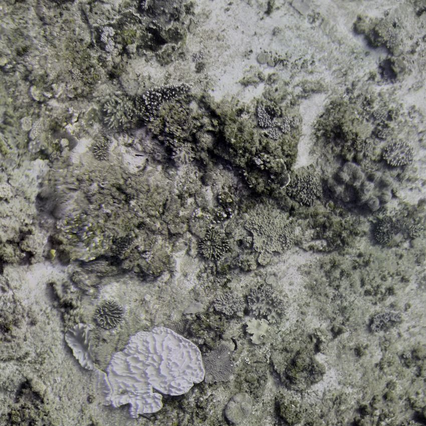
The International Archives of the Photogrammetry, Remote Sensing and Spatial Information Sciences, Volume XLII-2/W10, 2019
       Underwater 3D Recording and Modelling “A Tool for Modern Applications and CH Recording”, 2–3 May 2019, Limassol, Cyprus

 Figure 2. (Right) Bounding box of a coral in the ortho-mosaic
  map. (Left) Cropping Windows for the oversampling in data
  space; the points indicate the centers of such windows. This
      coral will be replicated 9 times in the final dataset.

cases, the two windows might be divided into smaller areas with
separate scores, and then re-combined to reach a properly bal-
anced set.

2.2    Corals Oversampling

The dataset used for the tests, as many other datasets of this type,
only contains a small number of representatives for the species
under monitoring, compared to the extension of the surveyed
area. This causes a significant problem of class imbalance when        Figure 3. An excerpt of the dataset after the coral oversampling.
training the network. To solve this issue, we propose a simple               (Top) RGB images. (Bottom) Corresponding labels.
oversampling strategy in data-space, based on the actual area cov-
erage of the specimens.                                                2.3   Re-assembling the output of the CNN

We subdivide each annotated coral into a set of overlapping sub-       Ideally, most of the CNN are translation-invariant because are
parts: the number of parts is proportional to the size the coral,      based on convolutional filters and max pooling layers. However,
while their arrangement follows the shape of the specimen. The         the padding operation in the convolutional filters introduces small
bounding box of each coral is regularly sampled, using as a step       but significant differences. In remote sensing applications, the
the average size of the smaller specimens: a cutting window is         size of the ortho-photo map is usually too large to be processed
applied on each of these sampled points. The size of the cutting       entirely with a single pass for memory constraints. In these cases,
window is determined by the size of the network training input         the segmentation is applied on an overlapping sliding window to
and by the maximum translation applied during the data augmen-         ensure the class consistency, in particular on the image borders.
tation. Each cropping window give us a new input image tile for        Since this approach produces more than one per-pixel classifi-
the input dataset. An example of the cropped tiles of a coral is       cation score, a method to re-assemble the segmented map is re-
shown in Fig. 2.                                                       quired.
This sampling produces a set of tiles that follow the size and
shape of the specimens, making possible to feed the network with       The standard method to obtain the final scores is to simply av-
all the coral borders, and to further apply a random-displacement      erage the overlapping results (Liu et al., 2017, Audebert et al.,
and/or rotation step of augmentation at training time, further in-     2017). Here, we propose to employ a method already used in
creasing the coral percentage.                                         multi-view stereo matching (Ma et al., 2017); using the Bayesian
                                                                       Fusion to aggregate the scores that belong to the same pixel.
This strategy is motivated by the presence of a very large num-
ber of small corals (which are therefore well represented in the       Defining SN = {s1 , s2 , . . . , sN } a set of classification scores
dataset), and only a few of large ones. Since we are working with      for a given pixel, generated by the sliding window in different
natural, growing structure, the idea is to give the same importance    positions, according to the Bayes rule we can write:
to small and large corals into the training and validation sets.
                                                                                                p(SN |y, SN −1 )p(y|SN −1 )
                                                                                   p(y|SN ) =                                          (1)
Classic feature-space oversampling are difficult to apply in this                                         p(SN )
specific case, because the pre-trained CNNs typically employed         where y is the output of the network for that pixel. By assuming
for features extraction are trained on dataset that does not con-      that the scores are i.i.d, it is possible to write:
tain this type of visual data. Additionally, standard augmentation
alone would not be able to take into account the spatial continuity                                         N
                                                                                                            Y
of the larger individuals and not guarantee to cover all the corals                      p(y|SN ) = µp(y)          p(si |y)            (2)
border. Working with ortho-mosaic makes this processing step                                                 i=1
possible, as the ground sampling distance is known, and larger
specimen are not scattered across multiple photos but are repre-       where µ is a constant. At this point, the final Bayesian aggrega-
sented by a single area on the map.                                    tion becomes:
                                                                                                                     N
                                                                                                                     Y
Figure 3 shows a dataset sample, largest coral appears several                    p(y = 0|SN )     =    p(y = 0)           p(si |y)
time in different position into the cropped area.                                                                    i=1

                                                 This contribution has been peer-reviewed.
                    https://doi.org/10.5194/isprs-archives-XLII-2-W10-151-2019 | © Authors 2019. CC BY 4.0 License.                    153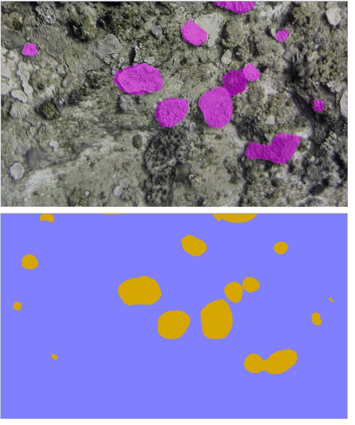
The International Archives of the Photogrammetry, Remote Sensing and Spatial Information Sciences, Volume XLII-2/W10, 2019
    Underwater 3D Recording and Modelling “A Tool for Modern Applications and CH Recording”, 2–3 May 2019, Limassol, Cyprus

                                             N
                                             Y
           p(y = 1|SN )      =    p(y = 1)         p(si |y)      (3)
                                             i=1

Note that p(y = 0|SN ) and p(y = 1|SN ) should be normalized
to obtain the probability that the pixel belongs to the species of
interest or not.

An interesting aspect of this formulation is that it includes the a
priori probabilities of the presence of the species of interest: i.e.
if we know in advance that, in the surveyed area, the coverage of
the species is not more than the X% of the seabed, it is possible
to take into account this information, and produce more reliable
scores for the pixels with an uncertain prediction (probabilities
close to 0.5).

       3. VALIDATION OF THE SEGMENTATION

The human error in labeling specimens adds uncertainty both at
the training phase and at the testing of the network. This lack of
consistency depends on the operator’s experience in distinguish-
ing exactly those types of marine organisms but also on the repet-
itiveness of the task. In (Beijbom et al., 2015), authors show           Figure 5. The Mozambique geo-referenced ortho-mosaic with
that the expert introduce an intra-annotator error of about the         the corresponding polygonal labels. On right, some examples of
10 − 11%. With the aim to reduce such source of errors we pro-                                annotated corals.
posed an interactive validation tool (implemented in PyQt) that
                                                                        The ortho-mosaic, generated with Agisoft PhotoScan, was built
allows the user to confirm, reject or copy an existing annotation
                                                                        from color-corrected images. For this purpose, we employed a
with a single click.
                                                                        combination of the CLAHE algorithm (Zuiderveld, 1994) in the
The tool interface is shown in figure 4. In the Comparison Panel,       Lab color space with a successive small auto adjustment of the
the two main windows, allow the user to analogize the original          RGB components. This global color adjustment works very well
human annotation (on the left) with the network predictions (on         in our case, the mean value of the images extracted from the
the right). The Navigation Panel, in the top-right, enable to reg-      ortho-mosaic for the training is always close to middle gray.
ister the actions performed within the map.
                                                                        We only have a single labeled coral class, the Soft Coral Dig-
This tool can be used in two different ways. It is possible to work
                                                                        itate, which shows a large intraspecific morphological variance
on the classification output of the network applied to an unseen
                                                                        (see Fig. 5) and covers approximately just the 6.4% of the seabed.
area, in order to efficiently correct erroneous predictions, calcu-
                                                                        The ’other’ class contains elements that are poor in features, such
lating at the same time the adjusted percentage of abundance and
                                                                        as sand, but also other corals classes morphologically similar to
coverage of the species. However, it is also possible to use it to
                                                                        the monitored class, which are thus excellent candidates to be
check the classification output of the network when applied on
                                                                        false positives. Our labels are loosely-fitting polygons surround-
the entire input dataset: in this case, it allows to quickly correct
                                                                        ings the corals, marked on a separate layer using QGIS, not fully
the errors in the input annotations, by comparing the results with
                                                                        coherent with their edges (see Fig. 5). However, this annotation
the original labels. At this point, a more correct labeling might
                                                                        technique is very fast and probably the most suitable in relation
be exported and used to re-train the network.
                                                                        to the smooth appearance of our data.

                                                                        4.1   Network and training parameters

                                                                        We do our experiments using a standard pre-trained CNN ar-
                                                                        chitecture for semantic segmentation tasks, the Bayesian Seg-
                                                                        Net (Kendall et al., 2015). Dataset tiles are pre-processed by
                                                                        subtracting the mean value, no further normalization are required
                                                                        thanks to the previous color adjustment. The fine-tuning of the
                                                                        network is obtained using an initial learning rate of 5 · 10−5 . This
                                                                        learning rate is reduced by a factor 5 every 50 epochs, for a total
                                                                        of 150 epochs. The optimizer is Adam with a small weights L2
      Figure 4. The semantic segmentation validation tool.              regularization (0.0005). Higher values of the regularization tends
                                                                        to oversmooth the coral borders.

                          4. RESULTS                                    Each input images is a tile of the ortho-map of 448 × 448 pix-
                                                                        els (two times the input size of the pre-trained SegNet). We used
We test our strategies on a 150 × 50 meters wide ortho-mosaic of        an image of such size to permit large translation during the data
the barrier reef already investigated in (Palma et al., 2017), con-     augmentation. In particular, each input tile is randomly flipped
taining various coral species, as well as rocks and sand regions,       horizontally and/or vertically, translated in a range of ±50 pix-
labeled by a single biologist (see Fig. 5). One pixel of the ortho-     els, and rotated in a range of ±10 degrees. The augmented im-
photo map covers around 1.14mm.                                         age is cropped centrally to obtain the input size of the network

                                                This contribution has been peer-reviewed.
                   https://doi.org/10.5194/isprs-archives-XLII-2-W10-151-2019 | © Authors 2019. CC BY 4.0 License.                       154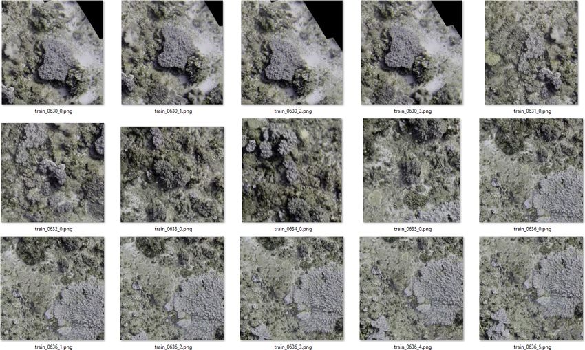
The International Archives of the Photogrammetry, Remote Sensing and Spatial Information Sciences, Volume XLII-2/W10, 2019
Underwater 3D Recording and Modelling “A Tool for Modern Applications and CH Recording”, 2–3 May 2019, Limassol, Cyprus
Figure 6. A dataset tile (Left), the probability map (Center),
cross-entropy mask (Right)
(224 × 224). We decided for these augmentation parameters
after some empirical tests. The batch size used is 32.
The architecture follows the typology of the input labeling. The
Bayesian Segnet, returns homogeneous regions predictions, i.e.
blobs, that are suitable to approximate the polygonal annotation.
However, coral colonies borders are generally jagged: more re-
cent architectures, such as DeepLabV3+ (Chen et al., 2018), could
be used to obtain a more precise per-pixel labeling.
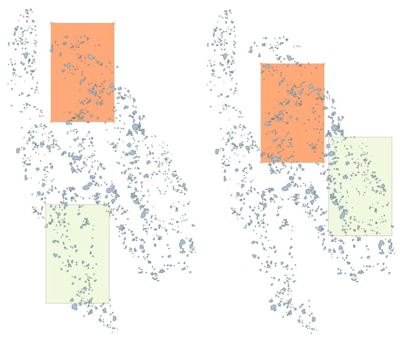
Figure 7. The Random Window dataset (on the left) and the
Strategies to deal with the inaccurate labeling of the polyg- Selected Windows dataset (on the right). Orange and Olive color
onal annotations. Polygonal annotation of corals is more ac- indicate respectively the validation and the test Area.
curate then the one based on points, but some labeling prob-
SCD Class Other Class
lems still remain. Coral contours are often too irregular to be Dataset
(predicted) (predicted)
annotated with a simple polygon, and on high-resolution ortho-
SCD Class 0.511 0.489
mosaics, texture artifacts may appear in correspondence of depth Random Windows
Other class 0.027 0.973
discontinuities. To deal with this problems, we tested two differ-
ent strategies to deal with the uncertainty around corals borders. SCD Class 0.585 0.415
Selected Windows
Other class 0.029 0.971
In the first strategy, probability maps are calculated by individu- Random Windows SCD Class 0.872 0.128
ally rasterizing each label, and applying a gaussian filter with a + Weighted Other Class 0.146 0.854
kernel of 20 pixels (σ = 5 pixels) to smooth out its borders. The
Selected Windows SCD Class 0.881 0.119
idea is to treat the labels as probability maps, with probability to
+ Weighted Other class 0.104 0.896
have coral equals to 1.0 when inside the corals, but with a de-
creasing ramp to 0.0 across the area of the border (see Fig. 6). In Table 1. Confusion matrices for the biologically-inspired
this case a binary cross-entropy loss is used. selection and random selection.
In the second strategy, the rasterized labels are thresholded to
added in an additional information channel to train the network.
carve out a thin mask covering the area across the border such
The Bayesian Segnet that we used for our tests was pre-trained
that the thickness of the mask is proportional to the size of the
with three channels, but we reserve to try this approach with a
coral (see Fig. 6). This time we decided to exclude the borders
multi-channel network because it seems very promising.
from the loss calculation. The rationale is try to learn the inner
region of specimens, i.e. the “inner patterns” of the corals. This 4.2 Biologically-inspired dataset partition
time we chose a cross-entropy loss function because we are deal-
ing with binary maps. The adaptive masking is necessary to pre- We used our area selection method, based on the spatial analysis
vent loosing too much useful data on small corals. In our dataset, of the populations, to identify the best training, validation and test
we set the minimum thickness to 7 pixels and a maximum one of area. These areas are shown in Figure 7. The obtained S scores
about 15-16 pixels. are 5.1, 5.5 and 5.8 for the test, validation and training dataset
respectively. This means that the descriptive statistics of these
According to our tests we can state that the second solution is areas are all quite close to one another, as we wanted.
inefficient. The network is not able to segment the coral borders
properly; the learned “inner patterns” does not guarantee better From now on, we will refer to the dataset obtained by splitting the
precision w.r.t. the whole polygonal labeling. Conversely, the tiles into training, validation and test sets using the areas selected
solution based on treating labels as probability maps and adding with our method as Selected Windows. Similarly, we will refer
an uncertain field around the borders is able to reduce the FPR to with Random Windows to the dataset in which the tiles are split
about 0.8-1.0%. using randomly selected areas. In this case, the scores are a bit
This result, combined with the Bayesian Fusion (see Table 5), higher (around 20.0), i.e. the random areas are still quite similar
gives the best performance in terms of False Positive Rate (FPR), but not be as good as the ones chosen with our method.
i.e. 2.5%, w.r.t the network with the best accuracy (0.960 vs Tables 1 and 2 summarize the obtained results. The term ‘weighted’
0.962) and the best F1-score (0.641 vs 0.650). This result is very means that, to compensate the class imbalance, we also intro-
encouraging and worthwhile more investigation to better assess duced a weighted cross entropy loss with the weights set as the
its advantages. inverse of the class frequency.
In recent works, as in (Maninis et al., 2018), the uncertainty of the As performance metrics, we consider the overall accuracy and
sketch labels is solved by transforming them into heat maps, then the F1-score, that measures the test accuracy more efficiently in
This contribution has been peer-reviewed.
https://doi.org/10.5194/isprs-archives-XLII-2-W10-151-2019 | © Authors 2019. CC BY 4.0 License. 155
The International Archives of the Photogrammetry, Remote Sensing and Spatial Information Sciences, Volume XLII-2/W10, 2019
       Underwater 3D Recording and Modelling “A Tool for Modern Applications and CH Recording”, 2–3 May 2019, Limassol, Cyprus

      Dataset                           Accuracy      F1-Score                                                  SCD Class      Other Class
                                                                         Dataset
      Random Windows                     0.949         0.511                                                    (predicted)    (predicted)
      Selected Windows                   0.944         0.591             Random Windows         SCD Class          0.793          0.207
      Random Windows + Weighted          0.856         0.388             + Oversampling         Other class        0.064          0.926
      Selected Windows + Weighted        0.895         0.535             Selected Windows       SCD Class          0.809           0.191
                                                                         + Oversampling         Other class        0.044           0.956
  Table 2. Comparison of accuracy and F1-Score between the
                                                                         Selected Windows       SCD Class          0.826           0.174
     biologically-inspired selection and random selection.
                                                                         + Dense Overs.         Other class        0.048           0.952
uneven class distribution. To better assess the amount of coral
correctly classified w.r.t the Other class, we also report the corre-         Table 3. Comparison between selected and random areas.
sponding confusion matrices. Note that due to the strong imbal-          Dataset                                  Accuracy      F1-Score
ance of the classes, a small classification error on the Other class
                                                                         Random W. + Oversampling                  0.929         0.537
greatly increases the amount of incorrectly classified pixels.
                                                                         Selected W. + Oversampling                0.945         0.674
According to the metrics used the network trained using the Se-
                                                                         Selected W. + Dense Oversampling          0.943         0.670
lected Windows is able to classify correctly more SCD (58.5%
vs 51.1% of the Random Windows) with basically the same FPR.
                                                                         Table 4. Performance of the proposed oversampling approach.
As a matter of fact, it has the best F1-Score. The number of
tiles used for training with the Random Windows is greater than
                                                                        method to reduce such inconsistencies is to average the scores on
the Selected Windows (906 vs 820), however, the biologically-
                                                                        a set of overlapping window. Typical overlap values used are 50%
inspired selection still outperforms the random selection.
                                                                        or 75%. In the following, we compare the averaging of the scores
This result is significant, also considering that we are working on
                                                                        (after the Softmax layer) with our Bayesian Fusion approach.
a relatively regular colonies distribution: the Mozambique dataset
portrays a flat reef, without major slopes, located centrally inside    Figure 8 shows an example of output probabilities produced for a
the barrier and not subject to external currents. Tests conducted       single sliding window. As clearly visible, the proposed Bayesian
on other sets of Random windows with comparable scoring give            Fusion can produce scores that show less uncertainty with respect
similar qualitative results. The performances greatly degrades          to those produced by simply averaging the input. This reduces
when the Windows have much higher values of S, i.e. > 40.               the presence of ambiguous range values, i.e. around 0.4-0.6, and
Regarding the use of the weighted cross-entropy loss, the imbal-        helps to remove the smaller wrongly-classified SCD. The perfor-
ance of our test case is so severe (the number of pixels of the Soft    mance evaluated against the ground truth of the scores aggregated
Coral Digitate are about 6.4% of the entire ortho-map) that this        using the Bayesian Fusion are slightly better than the ones of the
standard technique is unable to produce good results (compare           scores aggregated with the simple average (see Table 5). Note
the F 1 − Score in table 2). This further motivates the use of our      that the overlap of 75% does reduce the performance, most prob-
oversampling strategy to reduce the imbalance problem.                  ably due to the weak labeling at the corals’ edge, that corresponds
4.3    Corals Oversampling                                              to the zone of high uncertainty. The role of the prior probabilities
                                                                        can be easily understood by taking a look at the confusion ma-
As already stated, our dataset is heavily unbalanced (6.4% of           trix reported in Table 6. Since we know that the presence of the
coral pixels according to the provided labeling information). Our       SCD has a low probability w.r.t the Other class, the effect of the
simple oversampling method (see Section 2.2) is able to feed the        Bayesian fusion is to make the coral classification more strict, but
network with an amount of coral pixels between the 35% and              at the same time the FPR is greatly reduced.
40% of the training dataset, making it balanced and increasing
the performance considerably.                                           4.5    Using the validation tool

Tables 3 and 4 report the results obtained on the Random Win-           We compared two successive annotations performed in QGIS by
dows and the Selected Windows dataset after our data balancing          the same biologist after a few months. The biologist needed ap-
step. The oversampling step during the corals cropping tiles is         proximately 25 hours to verify and correct the previous annota-
about 132 pixels, which corresponds to cover the area with a step       tion using QGIS. Employing the validation tool for executing the
of 16 cm in physical space. The Dense Oversampling test used a          same task, the biologist took only 9 hours (about 9.2 seconds per
step of 66 pixels, producing a higher number of cropped tiles for       instance).
the large corals. Note that this solution increases the True Pos-       Figure 10 shows in light blue the polygons annotated consistently,
itive Rate (TPR) and the accuracy significantly, outperforming          in dark blue the false negatives (labels missing in the first ses-
the class weighting. The best accuracy reach 94.5% with an F1-          sion), and in red the false positives (labels incorrectly classified
score of 0.674. Intuitively, a severe oversampling also introduces      in the first session). More accurate results about the validation
redundant data that does not improve the performance anymore;           tool performance are described in (Pavoni et al., 2019).
this can be seen by looking at results of the the dense oversam-
pling test.                                                                        Method      Overlap     Accuracy     F1-Score
Unlike doing a random augmentation, with this data oversam-                        Average      50%         0.958        0.640
pling approach we are sure to cover the area of each SCD in-                       Bayesian     50%         0.962        0.650
stance.                                                                            Average      75%         0.957        0.641
                                                                                   Bayesian     75%         0.959        0.644
4.4    Bayesian Fusion vs Standard Fusion

As described in Section 2.3, the classification of a large map          Table 5. Performance of the proposed Bayesian Fusion approach
generated by using a sliding window approach may cause prob-            vs the usual Averaging method. Prior probabilities are set 0.2 for
lems like inconsistent classification at tiles borders. The standard               the SCD class and 0.8 for the “other” class.

                                                 This contribution has been peer-reviewed.
                    https://doi.org/10.5194/isprs-archives-XLII-2-W10-151-2019 | © Authors 2019. CC BY 4.0 License.                     156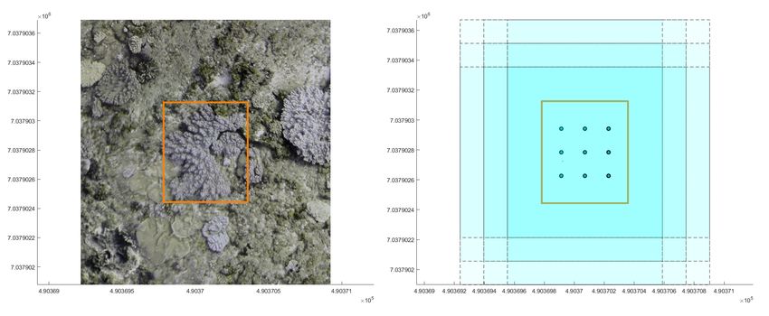
The International Archives of the Photogrammetry, Remote Sensing and Spatial Information Sciences, Volume XLII-2/W10, 2019
    Underwater 3D Recording and Modelling “A Tool for Modern Applications and CH Recording”, 2–3 May 2019, Limassol, Cyprus

 Figure 8. (From Left to Right) Input image. Manually annotated labels. Classification scores without aggregation. Average scores.
                                                        Bayesian Fusion.

                                  SCD Class      Other Class
     Method
                                  (predicted)    (predicted)
                   SCD Class         0.808          0.192
     Average
                   Other class       0.036          0.964
                   SCD Class         0.772          0.228
     Bayesian1
                   Other class       0.029          0.971
                   SCD Class         0.718          0.282
     Bayesian2
                   Other class       0.027          0.973

Table 6. Comparison between Averaging and Bayesian Fusion.
All methods use 50% overlap. Note that Bayesian1 corresponds
 to the prior probabilities set to 0.2 and 0.8 respectively, while
Bayesian2 corresponds to 0.1 and 0.9 (in this last case we have
              accuracy=0.960 and F1-score=0.639).

This time, we used the tool to validate the predictions with our
best performance network, Selected Windows + Oversampling +
Bayesian (50%), over the Test area. The biologist needed approx-
imately one hour to complete the task, with the following results:
                                                                            Figure 9. (Above) A close-up of the polygon labeled
  • 73 new instances, about the 15% of the Test area coral pix-              ortho-mosaic. (Below) The corresponding semantic
    els, were detected. Since coral instances are easily identified        segmentation obtained by our network on the Test area.
    when suggested by an automatic segmentation, this might
    justify the development of an assisted input tool.               In general, we can state that the overall performance of our net-
                                                                     work is in line or better than the current state of the art: an exam-
   • 40 small (about 10%) specimens predicted have not been          ple of a segmentation result is shown in (see Fig. 9). We point out
       validated because considered “uncertain”, confirming the com- that other similar solutions, without the described improvement
       plexity of the task.                                          strategies, requires larger dataset and more information to obtain
   • The FPR, that was about 2.9% in the confusion matrix, de-       similar quantitative performance, for example, the use of fluores-
       creased to 1.8% after the biologist validation.               cence data in addition to the RGB data by Alonso et al. (Alonso
                                                                     et al., 2017).
   • The TPR increased, in the same manner, from to 77.2% to
       81%.                                                          Regarding the proposed methods, the biologically-inspired dataset
                                                                     partition has demonstrated to work properly. We think it can be
                                                                     even more efficient with a higher number of classes and it can be
The new accuracy of the network, according with these values,        improved choosing more specific metrics for the specimen under
became 0.967.                                                        evaluation.
                                                                     According to the results, the oversampling strategies based on
4.6 Discussion and Qualitative Comparison
                                                                     size- and shape-driven cropping of the specimen has been very ef-
                                                                     fective to overcome the lack of data often characterizing this type
We report here a qualitative comparison with the work by King
                                                                     of study. The Bayesian Fusion has been able to obtain slightly im-
et al. (King et al., 2018) where the authors analyze several FCNN
                                                                     prove the performance w.r.t the standard averaging method. We
architectures in the task of semantic segmentation of coral reefs.
                                                                     underline that this strategy in general, and it can be applied also
In this field, making analogies with the performance of other su-
                                                                     in other monitoring applications based on ortho-photo maps.
pervised techniques is complicated by the lack of standard bench-
mark datasets. The input data are very similar to ours since the
different classes have been annotated directly onto an ortho-photo             5. CONCLUSIONS AND FUTURE WORK
map using a proprietary tool, but the SegNet has not been tested in
the comparison. The most promising network tested in (King et        In this paper, we presented a set of methods for the improvement
al., 2018), DeepLab v2, gives an accuracy of about 0.677 in clas-    of semantic segmentation of benthic communities using ortho-
sifying ten classes. We reached a maximum accuracy of 0.950 in       mosaic maps. The proposed strategies are automatic and ex-
classifying the Soft Coral Digitate class.                           ploit the characteristics of metricity and continuity of ortho-photo

                                                This contribution has been peer-reviewed.
                   https://doi.org/10.5194/isprs-archives-XLII-2-W10-151-2019 | © Authors 2019. CC BY 4.0 License.                   157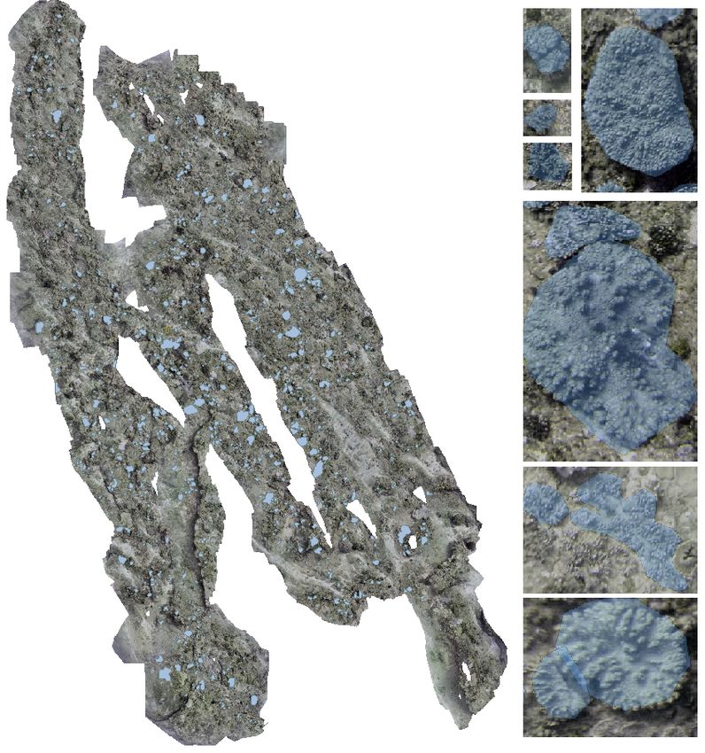
The International Archives of the Photogrammetry, Remote Sensing and Spatial Information Sciences, Volume XLII-2/W10, 2019
    Underwater 3D Recording and Modelling “A Tool for Modern Applications and CH Recording”, 2–3 May 2019, Limassol, Cyprus

                                                                                                  REFERENCES

                                                                         100 Islands Challenge Team, 2019. 100 Islands Challenge
                                                                         Project. http://100islandchallenge.org. Online; accessed 22
                                                                         February 2019.
                                                                         Alonso, I., Cambra, A., Muoz, A., Treibitz, T. and Murillo, A. C.,
                                                                         2017. Coral-segmentation: Training dense labeling models with
                                                                         sparse ground truth. In: ICCVW 2017, pp. 2874–2882.
                                                                         Audebert, N., Le Saux, B. and Lefèvre, S., 2017. Semantic seg-
                                                                         mentation of earth observation data using multimodal and multi-
                                                                         scale deep networks. In: S.-H. Lai, V. Lepetit, K. Nishino and
                                                                         Y. Sato (eds), ACCV 2016, pp. 180–196.
                                                                         Beijbom, O., Edmunds, P. J., Kline, D. I., Mitchell, B. G. and
                                                                         Kriegman, D., 2012. Automated annotation of coral reef survey
                                                                         images. In: CVPR2012, pp. 1170–1177.
                                                                         Beijbom, O., Edmunds, P. J., Roelfsema, C., Smith, J., Kline,
                                                                         D. I., Neal, B. P., Dunlap, M. J., Moriarty, V., Fan, T.-Y., Tan, C.-
                                                                         J., Chan, S., Treibitz, T., Gamst, A., Mitchell, B. G. and Krieg-
                                                                         man, D., 2015. Towards automated annotation of benthic survey
                                                                         images: Variability of human experts and operational modes of
                                                                         automation. PLOS ONE 10, pp. 1–22.
                                                                         Chen, L.-C., Zhu, Y., Papandreou, G., Schroff, F. and Adam, H.,
                                                                         2018. Encoder-decoder with atrous separable convolution for se-
                                                                         mantic image segmentation. In: ECCV.
                                                                         Edwards, C., Eynaud, Y., Williams, G. J., Pedersen, N. E.,
                                                                         Zgliczynski, B. J., Gleason, A. C. R., Smith, J. E. and Sandin,
                                                                         S., 2017. Large-area imaging reveals biologically driven non-
                                                                         random spatial patterns of corals at a remote reef. Coral Reefs
                                                                         36, pp. 1291–1305.
Figure 10. Human annotation errors. After a second annotation            Kendall, A., Badrinarayanan, V. and Cipolla, R., 2015. Bayesian
  session, some of the original labels were found to be false            segnet: Model uncertainty in deep convolutional encoder-decoder
          positive (red) or false negative (dark blue).                  architectures for scene understanding. CoRR.
                                                                         King, A., Bhandarkar, S. M. and Hopkinson, B. M., 2018. A
maps. The results of these solutions are encouraging, despite the        comparison of deep learning methods for semantic segmentation
low quality of the input at our disposal and despite the presence        of coral reef survey images. In: The IEEE Conference on Com-
of incorrect annotations.                                                puter Vision and Pattern Recognition (CVPR) Workshops.
The next step will be to test these methods on other datasets, con-
taining more classes and different information layers. We are cur-       Liu, Y., Minh Nguyen, D., Deligiannis, N., Ding, W. and
                                                                         Munteanu, A., 2017. Hourglass-shapenetwork based semantic
rently working on speeding up the human labeling step in order to        segmentation for high resolution aerial imagery. Remote Sensing.
obtain labels that better follows specimens border without com-
promising the advantages in terms of speed of the polygonal an-          Ma, L., Stueckler, J., Kerl, C. and Cremers, D., 2017. Multi-view
notation. More accurate labeling would justify the choice of a           deep learning for consistent semantic mapping with rgb-d cam-
finer-grain segmentation network. One of the greatest advantages         eras. In: IEEE International Conference on Intelligent Robots
of working with ortho-mosaics coming from 3D reconstruction              and Systems (IROS), Vancouver, Canada.
of the seabed is the opportunity to adopt a multi-modal approach,        Mahmood, A., Bennamoun, M., An, S., Sohel, F., Boussaid, F.,
combining the depth from the DEM maps with the RGB value                 Hovey, R., Kendrick, G. and Fisher, R. B., 2016. Automatic an-
from the textures. This would make also the evaluation criterion         notation of coral reefs using deep learning. In: OCEANS 2016
more robust; different species thrive at different depth ranges.         MTS/IEEE Monterey, pp. 1–5.
                                                                         Maninis, K.-K., Caelles, S., Pont-Tuset, J. and Van Gool, L.,
Life beneath the surface is characterized by a marvelous variety         2018. Deep extreme cut: From extreme points to object segmen-
of animal and plant species. According to our experience, ev-            tation. In: Computer Vision and Pattern Recognition (CVPR).
ery team of biologists deals and needs to identify a very specific
class of organisms. A customizable detection tool, that includes         Palma, M. A., Casado, M. R., Pantaleo, U. and Cerrano, C., 2017.
all the steps from the annotation to the segmentation and to the         High resolution orthomosaics of african coral reefs: A tool for
                                                                         wide-scale benthic monitoring. Remote Sensing 9, pp. 705.
validation of the results (with a streamlined interface), is the final
purpose of our research activity.                                        Pavoni, G., Corsini, M., Palma, M. and Scopigno, R., 2019. A
                                                                         validation tool for improving semantic segmentation of complex
                                                                         natural structures. In: Eurographics 2019 - Short Papers (in
                   ACKNOWLEDGEMENTS                                      press).
                                                                         Zuiderveld, K., 1994. Graphics gems iv. Academic Press Pro-
This work was supported by the Marie Sklodowska-Curie Action,            fessional, Inc., San Diego, CA, USA, chapter Contrast Limited
Horizon 2020 within the project GreenBubbles (Grant Number               Adaptive Histogram Equalization, pp. 474–485.
643712).

                                                 This contribution has been peer-reviewed.
                    https://doi.org/10.5194/isprs-archives-XLII-2-W10-151-2019 | © Authors 2019. CC BY 4.0 License.                       158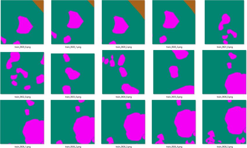
You can also read